Model of a Predictive Neural Network for Determining the Electric Fields of Training Flight Phases

Abstract

Tests on the content of the electrical component of the electromagnetic field (EMF) were carried out with an NHT3DL broadband meter by Microrad using a 01E (100 kHz ÷ 6.5 GHz) measuring probe. Measurements were made during training flights (Cessna C172, Cessna C152, Aero AT3, and Technam P2006T aircrafts). A neural network was used, the task of which was to learn to predict the successive values of average (E_RMS) and instantaneous (E_PEAK) electromagnetic fields used here. Such a solution would make it possible to determine the most favorable routes for all aircrafts. This article presents a model of an artificial neural network which aims to predict the intensity of the electrical component of the electromagnetic field. In order to create the developed model, that is, to create a training sequence for the model, a series of measurements was carried out on four types of aircraft (Cessna C172, Cessna C152, Aero AT3, and Technam P2006T). The model was based on long short-term memory (LSTM) layers. The tests carried out showed that the accuracy of the model was higher than that of the reference method. The developed model was able to estimate the electrical component for the vicinity of the routes on which it was trained in order to optimize the exposure of the aircraft to the electrical component of the electromagnetic field. In addition, it allowed for data analysis of the same training flight routes. The reference point for the obtained electric energy results were the normative limits of the electromagnetic field that may affect the crew and passengers during a flight. Monitoring and measuring the electromagnetic field generated by devices is important from an environmental point of view, as well as for the purposes of human body protection and electromagnetic compatibility. In order to improve reliability in general aviation and to adapt to the proposed requirements, aviation training centers are obliged to introduce systems for supervising and analyzing flight parameters.

1. Introduction

The current standards of pilot training lead to the constant pursuit of improving the level of safety. The European Aviation Safety Agency (EASA) takes extensive action to help control the critical components of the flight safety system, such as decreases in cognitive efficiency or spatial confusion among the aircraft crew. Moreover, there are reports in the literature of phenomena such as satiation syndrome and wrong prioritization among cabin crew. Even events of nonanthropogenic origin that happen in the background, resulting, for example, from rapid movement, have an impact on psychomotor variations and unconscious behavior among crew members [1,2]. The Pentagon research agency DARPA has proposed the hypothesis that these factors may contribute to class A accidents and deaths. There are also observations that the impact of semi-high frequencies can impair cognitive abilities [3,4]. Extensive electronic avionics systems are considered to be the source of fast-changing fields. These fields are also propagated from external sources, such as radio navigation systems or communication systems. The issue is of pivotal importance, given the interactions between these fields [5].

Artificial intelligence and neural networks have great potential to carry out detailed analyses regarding the recognition of aspects of flight parameters, such as forecasting the electric component (E) of the electromagnetic (EM) field. Effective parameter acquisition is essential for the neural network to function correctly. The form and length of training flights depend on the flight conditions, the flight phase and the location of the aircraft in real time. The values of the electromagnetic field may contain important information about the appropriate flight configuration, operation of avionic systems, radio navigation systems, the propulsion system itself, etc. [6,7].

In contemporary literature reports, there are lots of descriptions of a broad scope of neural network applications for the analysis of phenomena that are determined by many parameters. Examples include land communication, aviation, weather forecasting and health care. Various methods have been proposed in the literature to identify key parameters to help improve aviation safety [8,9].

Pytka et al. [10] showed the evolution of a convolutional neural network (CNN). The network was trained on the results of flight tests with a PZL 104 Wilga 35A aircraft. The distance of the tested aircraft from the ground when landing on a grass field was computed with the developed neural network model. Convolutional neural networks (CNNs) are among the various methods of deep learning with properties that particularly predispose them for the analysis of the movement of aviation objects.

An example of using a neural network to analyze a process with a great complexity of input data was described by Tomiło in [11]. A nonstandard architecture (roadNet) was used to identify the condition of the paving using an inertial measuring device (IMU) and a machine learning method. Using an artificial neural network (ANN), the highest precision of the validation set was obtained. Their tests showed that the ANN could classify the condition of the asphalt surface, and the developed system fulfills its task.

Kasprzyk [12,13] described the concept of predicting the speed of a vehicle using algorithms by means of neural networks and controlling the operation of a hybrid energy storage device in order to extend the life of lithium-ion cells. For this purpose, a series of measurements of driving speed and vehicle position on the same route and at similar times of day were carried out and then forecasted using a feedforward neural network (Levenberg–Marquardt algorithm) [12,13].

In their research, neural networks were used to study factors influencing, e.g., network carbon emissions [14]. Their article presents a systematic and versatile study on the optimization of a model in its current situation. Future development trends were discussed, taking into account factors influencing the implementation of green low-emission developments in China. For this purpose, a multivariate LSTM time series model and a CNN-LSTM model were used.

Yuanpeng Yang et al. [15] also described the results of using neural networks to analyze an electromagnetic field. Their article presents an EM long short-term memory neural network (EM-LSTMNN). A model was developed to speed up the calculations to accelerate radar cross-section (RCS) in optimizing low RCSs for high electrical uses. The described method converted traditional electromagnetic numerical calculations into an efficient numerical estimation using an LSTM neural network, resulting in a significant improvement in RCS computation speed. The performance of the proposed approach was indicated by comparing the RCS calculation score obtained through this method with those obtained by traditional EM simulation detection.

In the context of recognizing human activity, Ignatov [16] described an effective use of CNN. They discussed a user-agnostic approach to human activity classification based on deep learning. A CNN was used to extract local features, taking into account statistical features. This allowed for the preservation of information about time series globally. It has been demonstrated that the model used is characterized by high efficiency with relatively low computational costs and lack of manual feature engineering.

On the other hand, Ziyuan Guo et al. [17] sought to use (LSTM) networks to predict the propagation of the COVID-19 virus. They revealed that the developed artificial intelligence model can not only create strategies beneficial in the sector of public health but also optimize the allocation of resources.

Preethea et al. [18] used a neural network to forecast wind speed. The network identifies relevant spatial information to predict, e.g., wind speed. It has been demonstrated that, by using the CNN architecture, the effectiveness in capturing correlations and spatial patterns can be increased.

In order to guarantee efficient operation of urban rail transport, Jun Yang used convolutional neural networks to predict passenger flow in 2023. In his work, he proposes a method based on deep learning (ST-RAN). This method features high prediction accuracy and good applicability [19].

The described subject matter evolved from inspiration involving the possibilities of application of neural networks as presented in the cited works.

In this paper, we aim to extend our work [8]. The results of tests involving the intensity of the electrical component from navigation devices and systems, containing VHF omnidirectional radio range VOR, Instrument Landing System (ILS) and GPS, were presented in detail. In addition, we conducted a comparative analysis of the discussed radio systems to indicate the maximum values of the EMF coming from the analyzed sources. The result of the test revealed that the highest rate of the EMF component, which the pilot and crew are exposed to, comes from the VOR system. In 2019, the research team revised a publication [9] concerning the effect. Moreover, in 2019, the research team conducted research on the impact of mobile radio base stations (GSM and UMTS). It has been proven that the highest impact is caused by the GSM1800 system during a Cessna C152 flight.

The remainder of this paper has the following structure: Section 2 presents an overview of the E-field strength data received during measurements with the NHT3DL broadband meter with the 01E measurement probe and the statistical analysis of these data. A comprehensive description is provided of the model using the LSTM layer identifying characteristic flight parameters and predicting subsequent electromagnetic field values on selected aircraft routes. The description contains information about the developed structure of the ANN model, training model and validation process. The developed model was compared with the reference method. Section 3 discusses the neural network model used to predict the electric field strength during flights. It also presents an example of the model’s application, which can be used to determine the electric field strength of new routes existing in the vicinity of the training model flight route. Section 4 explains conclusions, limitations and future work.

2. Materials and Methods

Firstly, in order to create an artificial neural network model, in the first step, data in the form of electrical component of the electromagnetic field were collected (,) (E_PEAK, E_RMS) and GPS system indications for aircraft described in Section 2.1. They tested airplanes. The data were subjected to statistical analysis. Then, an artificial neural network architecture which uses the LSTM module was created. The neural network model was trained on the data and verified on a new data set after it was compared to the reference method—the naive method. Finally, simulations of the model’s indications were carried out on a new route, which is located in the area of the training model flight route. The described procedure is presented in Figure 1.

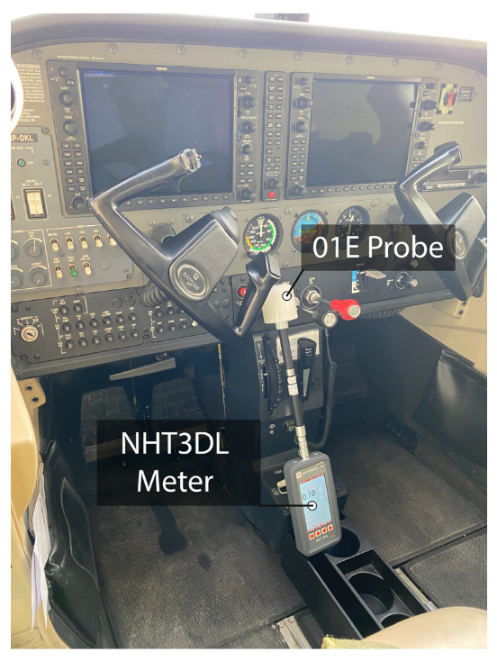
2.1. The Test Airplanes

Field strength measurements (E) were performed in four different aircrafts: Aero AT-3 R100, Cessna C172,Cessna C152, and Tecnam P2006T. The measurements were performed on the basis of the 2013/35/UE directive. It specifies measurement methods and assesses EMF at workplaces for the frequency ranging from 0 Hz to 300 GHz (Figure 2).

The Microrad EMF meter, model NHT3DL, is a portable signal analyzer in the frequency domain (1 Hz–1 MHz) and a broadband meter. The 01E probe is used to detect continuous wave (CW) and modulated signals for the frequency, ranging from 100 kHz to 6.5 GHz. Detailed technical parameters of the probe are presented in [8].

The airplanes are used on a daily basis for training flights in the Aviation Centre of The University College of Applied Science in Chelm, Poland. Individual aircrafts as well as their avionics and radio navigation systems were described by the author in the work [8]. In order to carry out the analysis (E), measurements were made during various flight routes. They lasted from 0.5 h to 4.6 h. In total, 12 flights were made, 3 flights per aircraft. The flights were carried out in Visual Metrological Conditions both day and night. To hold the consistency of the research methodology, radio navigation devices were used in accordance with a unified scheme. The measurement of the E-field strength is carried out in accordance with the three X.Y.Z axes. Particular attention is paid to the peak value of the impulse (PEAK), which defines the highest value recorded over time and the integrated value (RMS). The RMS value is used to assess the impact on humans. This is described in detail in INCNIRP 2020 [20]. Peak values, however, are more significant values in the context of electromagnetic compatibility (EMC), where the amplitude is important. According to standards and legislation, the RMS value is considered significant because it indicates the energy that is distributed through the field components in the context of a thermal phenomenon [9]. Measurements of key parameters started at the moment of taxiing and were carried out until stopping after landing. Taking into account the stochastic character, the sampling time was 1.

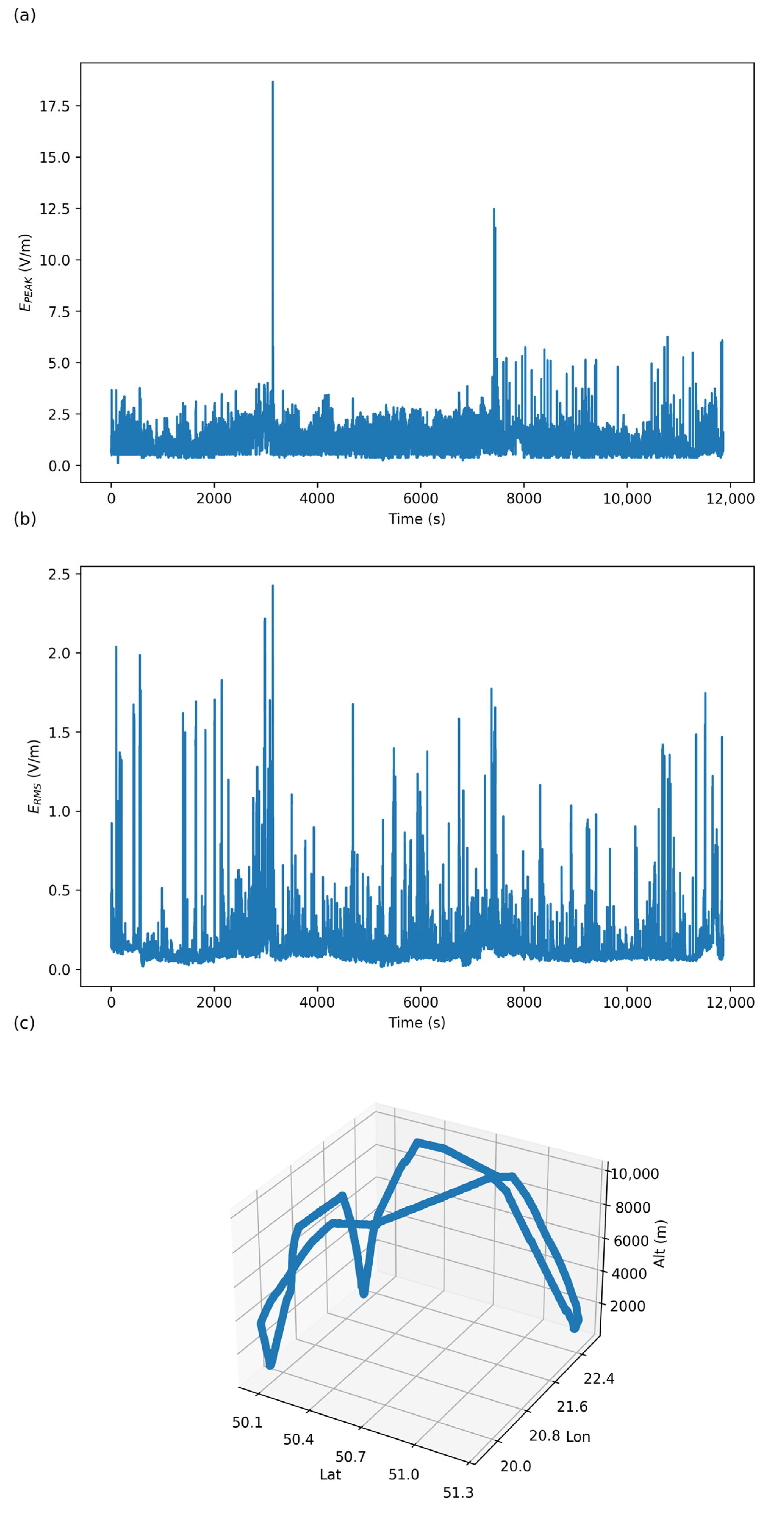
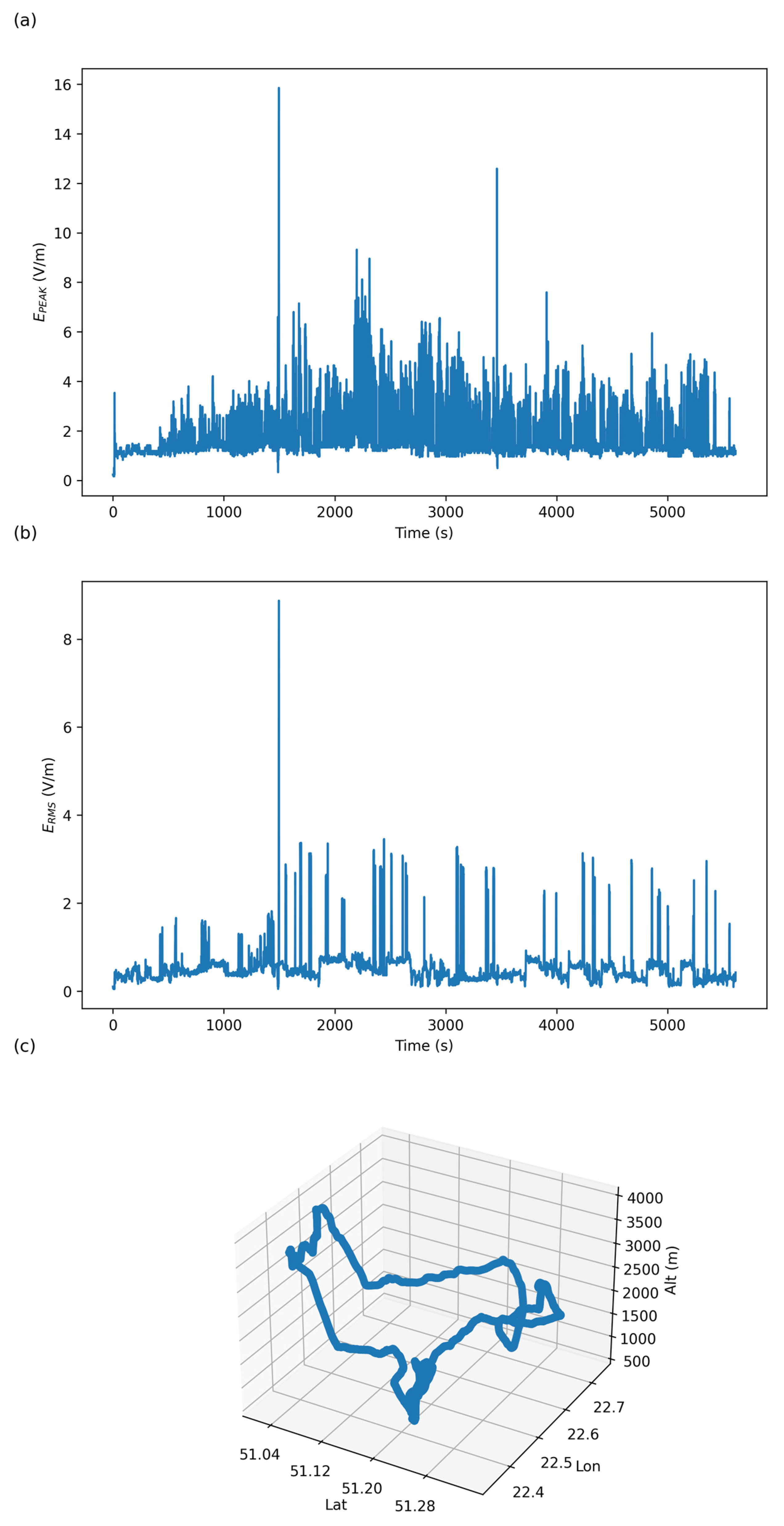
2.2. Overview of Measurement Data

Four models of aircraft, which are most commonly used in aviation, were selected for the measurements. The main parameters of the aircraft used are explained in [6]. The aircraft performed flights in accordance with standard operating procedures (SOP) approved for the purpose of conducting practical training at an Approved Training Organization. During the flights, key data acquisition was carried out, in particular, the value of the instantaneous electric component E_PEAK and the integral E_RMS. These parameters were supplemented with the instantaneous co-ordinates of the aircraft position in the space defined as latitude (Lat), longitude (Lon), and AltGPS. Values of field parameters were recorded using the NHT3DL meter by Microrad. The meter is equipped with a broadband measuring probe 01E (from 400 MHz to 6.5 GHz). Selected correlated parameters, which were related to the instantaneous co-ordinates of the location, are presented in the form of time courses in Figure 3, Figure 4, Figure 5, Figure 6, Figure 7, Figure 8, Figure 9 and Figure 10.

Based on the conducted tests, it can be noticed that the maximum electric field values for E_RMS = 8.959 V/m occur for Cessna C152 aircraft at an altitude of 894–1040 m above sea level. Subsequently, values of a similar order of E_RMS = 8.873 V/m were observed in the Aero AT3 aircraft when it was at a ceiling of 2220–2390 m above sea level. During measurements in the Tecnam P 2006 aircraft, the highest results were obtained E_RMS = 4.513 V/m at an altitude (770–933 m above sea level) similar to that for the Cessna 152. In the case of E_PEAK values, maximum results of 23.1 V/m were also observed for the Cessna C152 aircraft achieved when the aircraft was at an altitude of 1922–2069 m above sea level. Next, it can be observed that, in the case of Tecnam P2006, the maximum was 11.39 V/m and it was recorded at an altitude of 1910–2073 m above sea level. In the case of Aero AT3, the maximum measurement value was 15.85 V/m at an altitude of 2220–2390 m above sea level. In this case, the maximum values of E_RMS and E_PEAK were recorded at the same height. Maximum E_RMS and E_PEAK was also observed in case of Cessna C172 at an altitude of 9380–9842 m above sea level. The detailed origin of the increase in the maximum values of the E-field strength is described in [8].

The collected and analyzed data describe electromagnetic phenomena, the stochastic features of which are predisposed to create a model for learning neural networks. Experience in creating such networks of networks has shown that large data sets collected in various parameters are particularly conducive to creating adequate LSTM models.

Due to the stochastic nature of the experimental measurements and the large number of results received, a statistical analysis was carried out to identify regularities. Statistical variations (mean value, standard deviation (SD), and range of variability) of the electric field were estimated. The research assumed an inference error of 5 and significance level p < 0.05. The characteristics of electric field for selected flights are shown in

Table 1. Characteristic of E-field strength; V/m for testing airplane.

Nr Flights	Variable	Mean	SD	Maximum	Minimum
Type airplane	Cessna C172
1	EPEAK	1.398	0.714	18.66	0.103
2	EPEAK	2.003	0.942	11.33	0.495
3	EPEAK	1.518	0.617	6.893	0.234
1	ERMS	0.166	0.201	2.426	0.013
2	ERMS	0.226	0.229	2.156	0.055
3	ERMS	0.183	0.181942	1.966	0.054
Type airplane	Cessna C152
1	EPEAK	4.900	3.448	23.11	0.165
2	EPEAK	3.668	3.091	18.76	0.165
3	EPEAK	5.195	4.526	22.19	0.234
1	ERMS	0.911	1.188	8.959	0.014
2	ERMS	0.488	0.624	7.573	0.034
3	ERMS	0.717	0.7533	4.467	0.079
Type airplane	Aero AT3
1	EPEAK	1.919	1.152	15.85	0.165
2	EPEAK	1.766	1.372	12.51	0.333
3	EPEAK	2.265	1.439	10.95	0.165
1	ERMS	0.530	0.456	8.873	0.048
2	ERMS	0.584	0.936	5.240	0.070
3	ERMS	0.622	0.596	4.806	0.023
Type airplane	Tecnam P2006
1	EPEAK	0.928	0.4912	6.771	0.165
2	EPEAK	1.301	0.525	7.613	0.165
3	EPEAK	1.075	0.625	11.39	0.334
1	ERMS	0.145	0.130	2.833	0.054
2	ERMS	0.352	0.217	1.673	0.061
3	ERMS	0.172	0.150	4.513	0.047

.

The average E-field strength value for the analyzed airplanes ranges E_RMS from 0.145 to 0.911 V/m and E_PEAK from 0.928 to 5.195 V/m. Due to the large number of sources, the range of values obtained by measurement varies from E_RMS 0.013 V/m to 8.959 V/m and E_PEAK from 0.103 to 23.11 V/m.

Significant correlations observed between field values related to altitude for individual types of aircraft are shown in Figure 11, Figure 12, Figure 13 and Figure 14. The figures presented below should be interpreted as a matrix in which each cell shows its values from labels on the x and y axes. The ones with the same values are presented in the histogram.

Based on the analysis for the Cessna C 172 aircraft, it can be seen that high E_RMS values occur for altitudes up to 2000 m above sea level. The highest values appear at an altitude of 10,000 m above sea level. The maximum instantaneous electric field strength values appear for similar altitude levels as the integral values.

In the case of the Cessna 152 aircraft, as a result of the analysis, it can be seen that the highest integral values of the E component occur during the aircraft’s ascent to an altitude of 1000 m above sea level, while the maximum instantaneous values occur in the range from 2000 to 2500 m above sea level.

Importantly, during the flight with the Aero AT3 aircraft, the maximum levels of the instantaneous electric field values are observed at a similar level as in the case of the Cessna C152 aircraft; however, the maximum value is much lower. The E_RMS values during the climb of the aircraft are at a similar level. A significant growth in the intensity of the electric component was noticed at an altitude of 2500 m above sea level.

In the case of the Tecnam aircraft, the measured values of the electrical component increase both in average and instantaneous values for the altitude of 750 and 2000 above sea level. The obtained results are lower than those for the Cessna C152 and Aero AT3 aircraft.

As can be seen from the above dependencies, for certain altitude values, there are characteristic densified increases in the E_RMS and E_PEAK values. Histograms for selected measurements for the tested aircraft are presented in Figure 15 (E_RMS) and Figure 16 (E_PEAK).

For the Cessna C 172, the largest number of measurements reaches small values. Another set of values that have a high abundance is in the range of 1 to 3 V/m. In the case of the Cessna C152, the greatest value of the electric component of the electromagnetic field corresponds to values from 0 to 5 V/m. In the case of Aero AT3, the greatest value of the electric component of the electromagnetic field can be observed from 0 to 5 V/m. In the case of the Tecnam P2006 aircraft, the measured values obtained are similar to those of the Cessna C172 aircraft (from 0 to 3 V/m).

For the Cessna C 172, the largest number of measurements reaches small values ranging from 0 to 0.5 V/m. In the case of the Cessna C152, the greatest value of the electric component of the electromagnetic field corresponds to values from 0 to 2 V/m. In the case of Aero AT3, the range in which the value was most often recorded was in the range from 0 to 1 V/m. Tecnam P2006T and Cessna C172 airframes were characterized by similar ranges of measurement values.

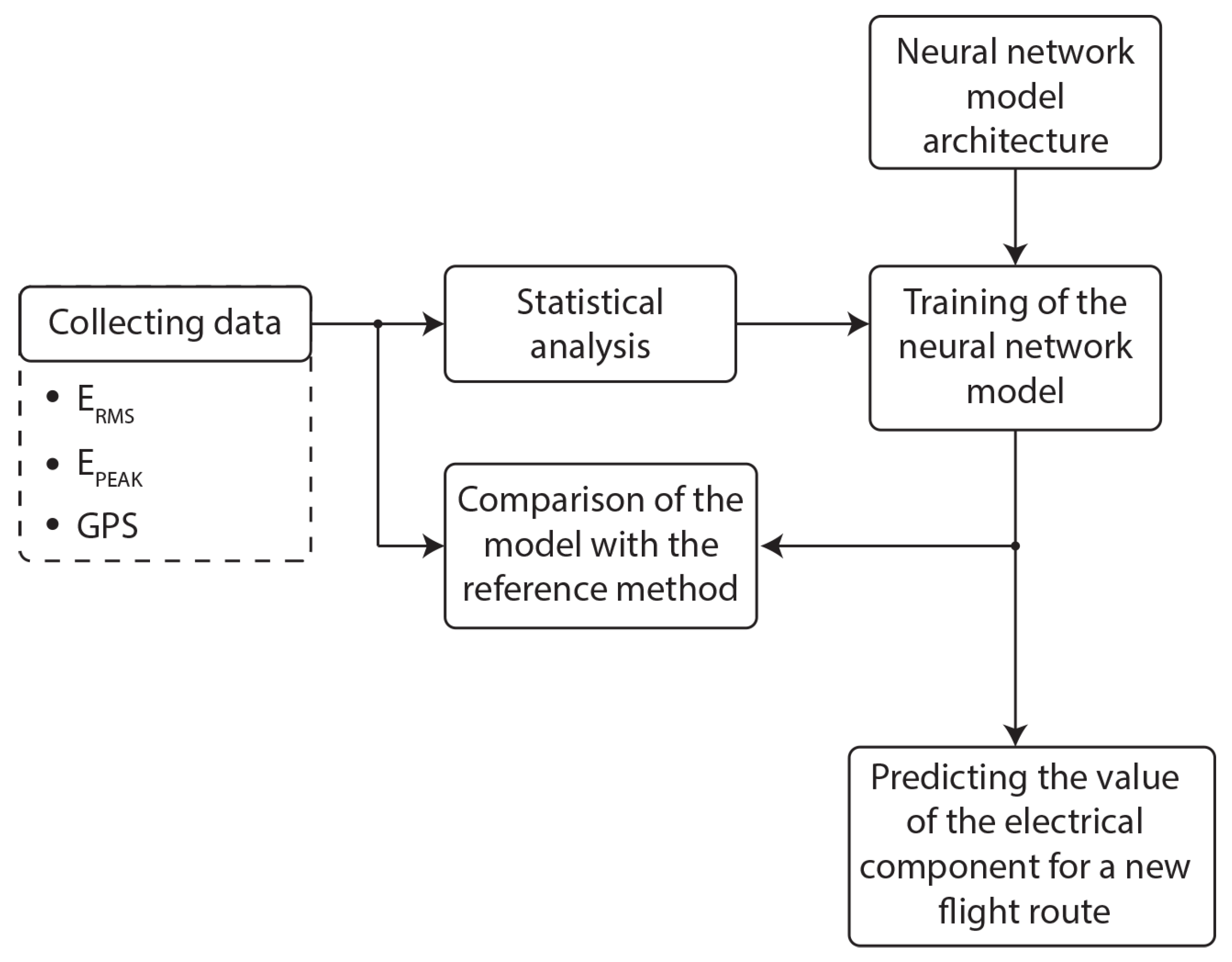
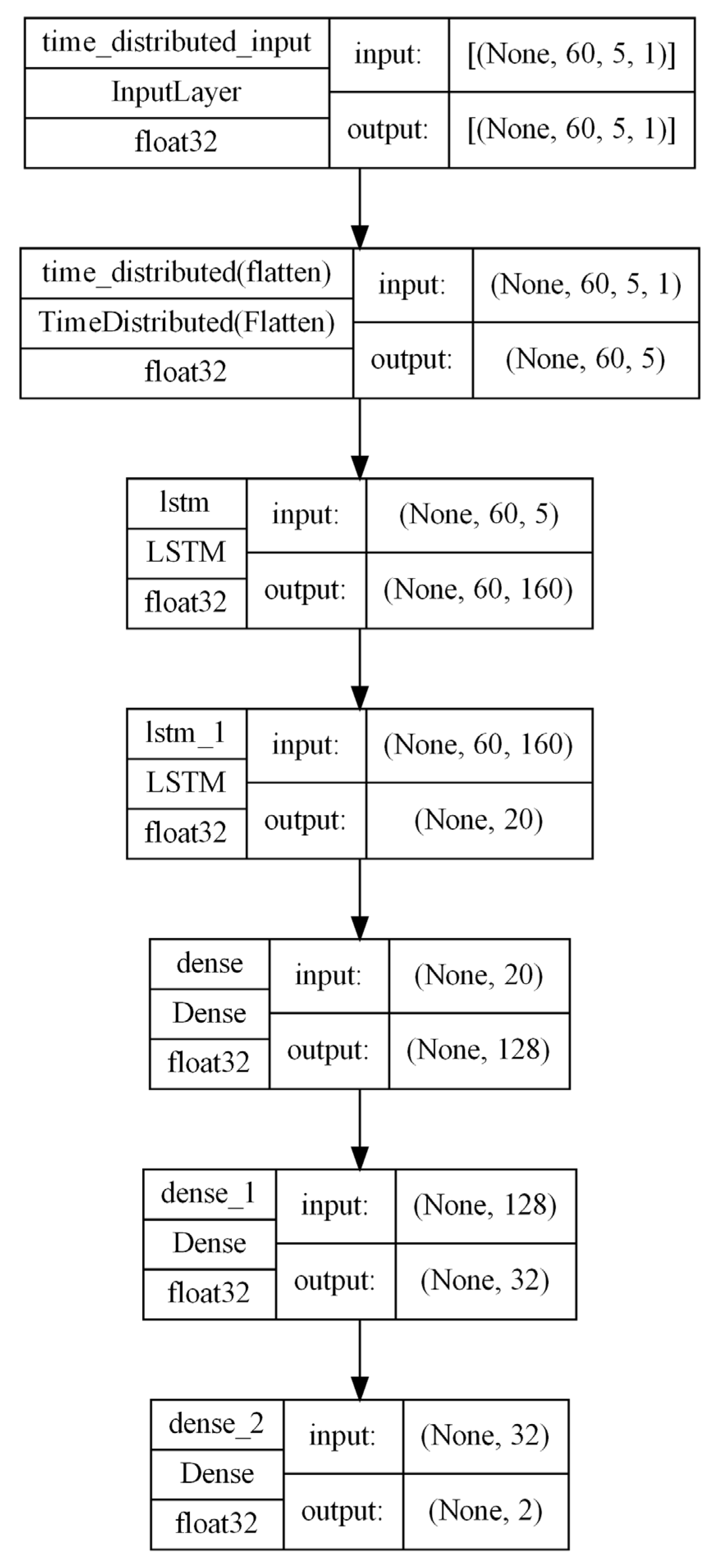
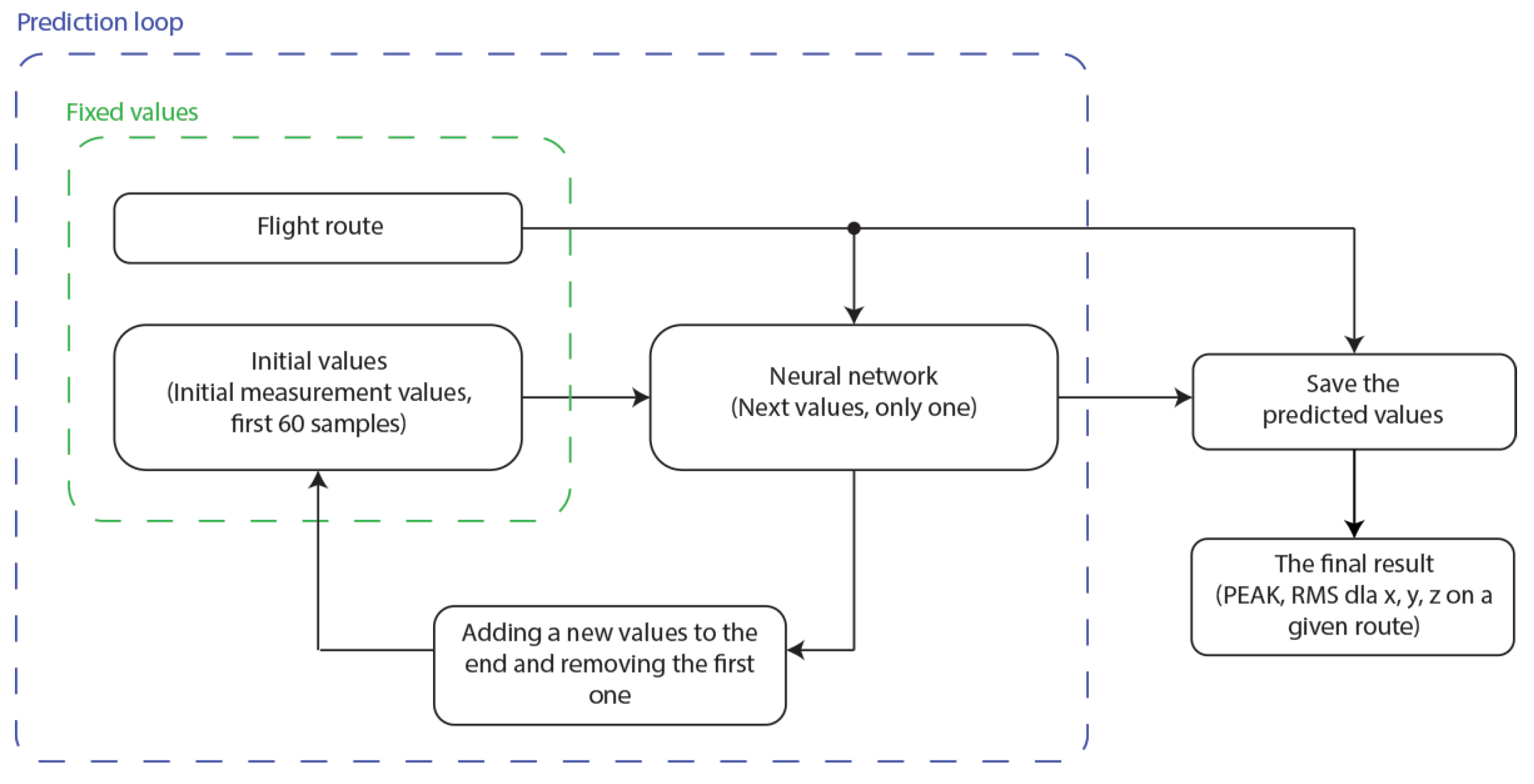
2.3. Development of the Artificial Neural Network Model

The LSTM model of the neural network was developed to recognize the correlation of the flight phases with the measured quality of the E-field strength. Waveforms of E-field strength were recorded during flights carried out as part of training flights. They were used to initiate and train a neural network.

In order to unify the results, a neural network was used, the task of which is to learn how to predict successive instantaneous maximum and integral values of the electromagnetic field. Such a solution will make it possible to establish a uniform route for all aircrafts. This will allow for the selection of a favorable route with a reduced level of electric field intensity.

In the LSTM layer, the output depends on 3 main elements: input data at current time step, cell state—current long-term memory, and hidden state—output at the previous point in time. In the LSTM layer, gates are used, which are responsible for the way information enters the layer, how it is stored in it, and how it leaves the layer. For a given timestamp $t$, the input data to the layer are cell state $C_{t-1}$ and hidden state $h_{t-1}$ and input data $x_t$. These data are processed by the forget gate, where it is decided which elements of $C_{t-1}$ are useful (for each element of $C_{t-1}$, weights are assigned) based on $h_{t-1}$ and $x_t$. The next step is called the input gate. This step sets which new information should be added to the cell state. The output from the LSTM layer is the newly updated cell state $C_t$ and new hidden state $h_t$. The output gate is used to assign new weights to $h_t$ by using $C_t$. The detailed principle of operation of the LSTM network is presented in [21,22,23,24,25].

The developed model of the neural network consists of 7 layers, which include:

• Time-distributed input layer, whose task is to prepare input data to pass through LSTM cells;
• The flattening layer changes the dimension of the input data matrix to the format 1 to x, where x is the total number of all cells in the matrix;
• The task of the 2 layers of LSTM allows for proper storage of values from previous cycles;
• Three fully connected layers of neurons are responsible for creating a hyperplane for the data and the appropriate selection of output values, in this case, E_RMS and E_PEAK.
• The network model is shown in Figure 17.

A predictive model using artificial neural networks was proposed (Figure 18). The model accepts the flight route as input values and analyzes the indications of the instantaneous and integral electric field strength values resulting from the recorded experimental studies. The model performs an iterative analysis by adding a new value to the analyzed window, which results in electric field strength values for given geographic co-ordinates.

The artificial neural network model was trained using the Adam algorithm with the following parameters:$\alpha =0.001;{\beta }_1=0.9, {\beta }_2=0.999; ϵ={10}^{-8}$, according to [25]. For each aircraft separately, a new neural network model with the structure described previously was created. The target number of epochs was 300. The mean absolute error (MAE) was assumed as the loss function. In the learning process, the highest value of the loss function fell on the validation set in the Cessna 152 aircraft and amounted to 0.0672, while the lowest value of the loss function fell on the set for teaching the Tecnam P2006T aircraft and amounted to 0.009. Figure 19 shows the course of the neural network learning process.

In order to verify the model for each of the tested aircraft, it was decided to compare the mean square error (MSE) metric for the input data against the developed artificial neural network model and the naive method. For each aircraft, the neural network model predicts values with greater accuracy than the naive method.

Table 2. Comparison of the winding method with the developed artificial neural network model of the obtained electric field values (E, V/m).

Aircraft	Variable	Method
		Naive	ANN
Aero AT3	EPEAK (V/m)	2.0215	1.9696
	ERMS (V/m)	2.0107	1.4034
Cessna 152	EPEAK (V/m)	4.6422	4.4642
	ERMS (V/m)	3.0470	2.1128
Cessna 172	EPEAK (V/m)	1.4372	1.4152
	ERMS (V/m)	1.6824	1.1988
Tecnam P2006T	EPEAK (V/m)	1.0983	1.0950
	ERMS (V/m)	1.4821	1.0464

shows a comparison of the winding method with the developed artificial neural network model.

Based on the developed model of the ANN, an experiment was carried out in which the flight route shown in Figure 20 was adopted. The dot marked in Figure 20 represents the take-off point of the plane. The task of the model is to determine the indications of the electric field strength for the given route.

The flight path was selected as part of a sinusoidal function in order to test the prediction of the value of the electric component of the electromagnetic field on a new, unknown route. The new path was selected so that its boundaries were within the range of data from aircraft flights. In order to make the analysis more detailed, the flight route is presented in 3D in Figure 21.

As a result of the collected measurement data, a neural network model was created that is able to predict changes in the electric field strength in the appropriate phases of flight 3.

3. Results and Discussion

The instantaneous and integral values of the measurements were superimposed on a grid with a cell size of 0.3 by 0.3 lat/lon to show field values along the route. The results using the neural network are presented successively in Figure 22, Figure 23, Figure 24 and Figure 25 for individual types of aircraft. The differences between the values for individual elements of the grid result from the fact that each model was trained on a different route, and the markings on the grid are relative to the origin of the co-ordinate system, which was determined by the lowest value from the location of the aircraft in the training sequence. To make it easier to distinguish values presented in the figures, they are marked in different colors (Figure 22, Figure 23, Figure 24 and Figure 25).

Table 3. Characteristics predictive of the intensity of the E component of the EMF energy (E, V/m) for new testing route.

Variable	Mean	SD	Maximum	Minimum
Cessna C172
EPEAK	1.945	1.294	12.317	0.354
ERMS	0.259	0.072	0.5011	0.042
Cessna C152
EPEAK	2.291	1.206	11.463	0.245
ERMS	1.755	0.829	5.786	0.310
Aero AT3
EPEAK	1.296	0.812	6.210	0.132
ERMS	1.709	0.936	6.789	0.337
Tecnam P2006
EPEAK	1.109	0.712	7.171	0.100
ERMS	0.875	0.400	3.016	0.165

shows the obtained results of the prediction for new testing route.

On the basis of the analysis, it can be seen that the characteristics obtained as a result of using the neural network model are close to the values obtained in experimental studies.

4. Conclusions

This article presents a model algorithm using neural networks for the analysis of key field parameters during flight phases. In the process of identification and subsequent learning of the network with the use of artificial intelligence, it obtained the expected prognostic capabilities for determining optimal flight routes.

Thanks to the development of the LSTM network model, trends were identified that correlate the detailed positions of aircraft with the measured E_RMS and E_PEAK values. Field mapping during flights is innovative, opens up new possibilities, and allows empirical study of fields that are of both natural and anthropogenic origin. Modeling with trained networks allows you to make field forecasts with high accuracy. The developed algorithm allows for quantitative and qualitative identification of hazards related to the exposure of people conducting pilot training.

The developed model has greater accuracy than the naive method. The developed model consists of 127,602 parameters and the processed data are time series; therefore, the model can be considered as not requiring large amounts of computational power.

The development of the neural network model algorithm will be used in further research as part of the flight route optimization. In addition, a method for predicting the E-field strength was developed by using an artificial neural network to determine optimal flight routes. It is worth noting that an increases in the accuracy of forecasting occurs with the collection of a larger set of training data.

References

1. Creating Breakthrought Technologies Capabilities for National Security. Available online: https://www.darpa.mil (accessed on 6 January 2022).
2. Xiong, G.; Przystupa, K.; Teng, Y.; Xue, W.; Huan, W.; Feng, Z.; Qiong, X.; Wang, C.; Skowron, M.; Kochan, O.; et al. Online Measurement Error Detection for the Electronic Transformer in a Smart Grid. Energies 2021, 14, 3551. [Google Scholar] [CrossRef]
3. Sun, L.; Qin, H.; Przystupa, K.; Majka, M.; Kochan, O. Individualized Short-Term Electric Load Forecasting Using Data-Driven Meta-Heuristic Method Based on LSTM Network. Sensors 2022, 22, 7900. [Google Scholar] [CrossRef] [PubMed]
4. Liyuan, S.; Yao, M.; Fei, G.; Yantao, D.; Cheng, G. Analysis of the Electromagnetic Environment in the Aircraft with Airborne VLF DTWA. In Proceedings of the 4th World Congress on Electrical Engineering and Computer Systems and Sciences (EECSS’18), Madrid, Spain, 21–23 August 2018. [Google Scholar]
5. Bakunowicz, J.; Rzucidło, A. Detection of Aircraft Touchdown Using Longitudinal Acceleration and Continuous Wavelet Transformation. Sensors 2020, 20, 7231. [Google Scholar] [CrossRef] [PubMed]
6. Krasuski, K.; Ćwiklak, J. Aircraft positioning using DGNSS technique for GPS and GLONASS data. Sens. Rev. 2020, 40, 559–575. [Google Scholar] [CrossRef]
7. Irfan, M.; Ayub, N.; Althobiani, F.; Ali, Z.; Idrees, M.; Ullah, S.; Rahman, S.; Alwadie, A.S.; Ghonaim, S.M.; Abdushkour, H.; et al. Energy theft identification using AdaBoost Ensembler in the Smart Grids. CMC-Comput. Mater. Contin. 2022, 72, 2141–2158. [Google Scholar] [CrossRef]
8. Michałowska, J.; Pytka, J.; Tofil, A.; Krupski, P.; Puzio, Ł. Assessment of Training Aircraft Crew Exposure to Electromagnetic Fields Caused by Radio Navigation Devices. Energies 2021, 14, 254. [Google Scholar] [CrossRef]
9. Michałowska, J.; Tofil, A.; Józwik, J.; Pytka, J.; Legutko, S.; Siemiątkowski, Z.; Łukaszewicz, A. Monitoring the Risk of the Electric Component Imposed on a Pilot During Light Aircraft Operations in a High-Frequency Electromagnetic Field. Sensors 2019, 19, 5537. [Google Scholar] [CrossRef] [PubMed]
10. Pytka, J.; Budzyński, P.; Tomiło, P.; Michałowska, J.; Gnapowski, E.; Błażejczak, D.; Łukaszewicz, A. IMUMETER—A Convolution Neural Network-Based Sensor for Measurement of Aircraft Ground Performance. Sensors 2021, 21, 4726. [Google Scholar] [CrossRef] [PubMed]
11. Tomiło, P. Classification of the Condition of Pavement with the Use of Machine Learning Methods. Transp. Telecommun. J. 2023, 24, 158–166. [Google Scholar]
12. Kasprzyk, L. Wybrane zagadnienia modelowania ogniw elektrochemicznych i superkondensatorów w pojazdach elektrycznych. Poznań Univ. Technol. Acad. J. Electr. Eng. 2019, 101, 3–55. [Google Scholar]
13. Burzyński, D.; Kasprzyk, L. A novel method for the modeling of the state of health of lithium-ion cells using machine learning for practical applications. Knowl.-Based Syst. 2021, 219, 106900. [Google Scholar] [CrossRef]
14. Chang, Z.; Jiao, Y.; Wang, X. Influencing the Variable Selection and Prediction of Carbon Emissions in China. Sustainability 2023, 15, 13848. [Google Scholar] [CrossRef]
15. Yang, Y.; Xinyang, S.; Wang, Q.; Fang, C. Enhancement of Electromagnetic Scattering Computation Acceleration Using LSTM Neural Networks. Electronics 2023, 12, 3900. [Google Scholar] [CrossRef]
16. Ignatov, A. Real-time human activity recognition from accelerometer data using Convolutional Neural Networks. Appl. Soft Comput. 2018, 62, 915–922. [Google Scholar] [CrossRef]
17. Guo, Z.; Lin, Q.; Meng, X. A Comparative Study on Deep Learning Models for COVID-19 Forecast. Healthcare 2023, 11, 2400. [Google Scholar] [CrossRef] [PubMed]
18. Preethaa, S.; Muthuramalingam, A.; Natarajan, Y.; Wadhwa, G.; Yusuf, A. A Comprehensive Review on Machine Learning Techniques for Forecasting Wind Flow Pattern. Sustainability 2023, 15, 12914. [Google Scholar] [CrossRef]
19. Yang, J.; Dong, X.; Yang, H.; Han, X.; Wang, Y.; Chen, J. Prediction of Inbound and Outbound Passenger Flow in Urban Rail Transit Based on Spatio-Temporal Attention Residual Network. Appl. Sci. 2023, 13, 10266. [Google Scholar] [CrossRef]
20. RF EMF Guidelines 2020. Available online: https://www.icnirp.org/en/activities/news/news-article/rf-guidelines-2020-published.html (accessed on 1 January 2023).
21. Krasuski, K.; Wierzbicki, D. Monitoring Aircraft Position Using EGNOS Data for the SBAS APV Approach to the Landing Procedure. Sensors 2020, 20, 1945. [Google Scholar] [CrossRef] [PubMed]
22. Sezer, A.; Altan, A. Detection of solder paste defects with an optimization-based deep learning model using image processing techniques. Solder. Surf. Mt. Technol. 2021, 33, 291–298. [Google Scholar] [CrossRef]
23. Sezer, A.; Altan, A. Optimization of deep learning model parameters in classification of solder paste defects. In Proceedings of the 2021 3rd International Congress on Human-Computer Interaction, Optimization and Robotic Applications (HORA), Ankara, Turkey, 11–13 June 2021. [Google Scholar]
24. Kinga, D.; Ba, J. Adam: A method for stochastic optimization. In Proceedings of the 3rd International Conference for Learning Representations, San Diego, CA, USA, 7–9 May 2015. [Google Scholar]
25. Elsworth, S.; Güttel, S. Time Series Forecasting Using LSTM Networks: A Symbolic Approach. arXiv 2020, arXiv:2003.05672. [Google Scholar]
Figure 1. Research method.
Energies 17 00126 g001
Figure 2. Measurement system installed in a Cessna C172 aircraft.
Energies 17 00126 g002
Figure 3. Example of measurement of the E component of the EMF in the time function for Cessna C172 flight nr 1: (a) change in EPEAK value over time 1; (b) change in ERMS value over time 2; (c) flight trajectory.
Energies 17 00126 g003
Figure 4. Example of measurement of the E component of the EMF in the time function for Cessna C172 flight nr 2: (a) change in EPEAK value over time 1; (b) change in ERMS value over time 2; (c) flight trajectory.
Energies 17 00126 g004
Figure 5. Example of measurement of the intensity of the E component of the EMF in the time function for the Cessna C152 flight nr 1: (a) change in EPEAK value over time 1; (b) change in ERMS value over time 2; (c) flight trajectory.
Energies 17 00126 g005
Figure 6. Example of measurement of the intensity of E component of the EMF in the time function for Cessna C152 flight nr 2: (a) change in EPEAK value over time 1; (b) change in ERMS value over time 2; (c) flight trajectory.
Energies 17 00126 g006
Figure 7. Example of measurement of the intensity of the E component of the EMF in the time function for Aero AT3 flight nr 1: (a) change in EPEAK value over time 1; (b) change in ERMS value over time 2; (c) flight trajectory.
Energies 17 00126 g007
Figure 8. Example of measurement of the intensity of the E component of the EMF in the time function for Aero AT3 flight nr 2: (a) change in EPEAK value over time 1; (b) change in ERMS value over time 2; (c) flight trajectory.
Energies 17 00126 g008
Figure 9. Example of measurement of the intensity of the E component of the EMF in the time function for Tecnam P2006 flight nr 1: (a) change in EPEAK value over time 1; (b) change in ERMS value over time 2; (c) flight trajectory.
Energies 17 00126 g009
Figure 10. Example of measurement of the intensity of the E component of the EMF in the time function for Tecnam P2006 flight nr 2: (a) change in EPEAK value over time 1; (b) change in ERMS value over time 2; (c) flight trajectory.
Energies 17 00126 g010
Figure 11. Correlations between the obtained values characterizing the field sizes in relation to the altitude for the Cessna 172.
Energies 17 00126 g011
Figure 12. Correlations between the obtained values characterizing the field sizes in relation to the altitude for the Cessna 152.
Energies 17 00126 g012
Figure 13. Correlations between the obtained values characterizing the field values in relation to the altitude for Aero AT3.
Energies 17 00126 g013
Figure 14. Correlations between the obtained values characterizing the field quantities in relation to the altitude for Tecnam P2006T.
Energies 17 00126 g014
Figure 15. Histogram for the obtained measurement values of integrals electric field strength (ERMS) for individual tested aircraft.
Energies 17 00126 g015
Figure 16. Histogram for the impulse electric field strength measurement (EPEAK) values obtained for each tested aircraft.
Energies 17 00126 g016
Figure 17. Model of structure of the data used for network.
Energies 17 00126 g017
Figure 18. A predictive model.
Energies 17 00126 g018
Figure 19. The process of learning a neural network.
Energies 17 00126 g019
Figure 20. Comparative route—top view.
Energies 17 00126 g020
Figure 21. Comparative route—spatial projection.
Energies 17 00126 g021
Figure 22. Strength of E-field in time function for prediction round of Cessna C172 airplane.
Energies 17 00126 g022
Figure 23. Strength of E-field in time function for prediction round of Cessna C152 airplane.
Energies 17 00126 g023
Figure 24. Strength of E-field in time function for prediction round of Aero AT3 airplane.
Energies 17 00126 g024
Figure 25. Strength of E-field in time function for prediction round of Tecnam P2006 airplane.
Energies 17 00126 g025