Simulation of the Asphaltene Deposition Rate in Oil Wells under Different Multiphase Flow Condition

Abstract

As the wellbore pressure falls below the bubble point pressure, the light components in the oil phase are liberated, forming additional vapor, and the single-phase flow becomes a gas–liquid two-phase flow. However, most studies simplify the multiphase flow to a single-phase flow to study asphaltene deposition in wellbores. This assumption under multiphase conditions may lead to inaccurate prediction results and a substantial economic and operational burden for the oil and gas industry. Therefore, it is crucial to predict the deposition rate of asphaltene in a multiphase flow to assist in minimizing this issue. To do so, the volume of fluid coupling level-set (VOSET) model was used to obtain the flow pattern (bubble, slug, churn, and annular) in the current work. In the next step, the VOSET + k-ε turbulent + DPM models were used to simulate asphaltene deposition in a multiphase flow. Finally, the effects of different parameters, such as the gas superficial velocity, liquid superficial velocity, particle diameter, interfacial tension, viscosity, and average deposition rate, were investigated. The findings revealed that the maximum average deposition rate of asphaltene particles in a bubble flow is 1.35, 1.62, and 2 times that of a slug flow, churning flow, and annular mist flow, respectively. As the apparent velocity of the gas phase escalates from 0.5 m/s to 4 m/s, the average deposition rate experiences an increase of 82%. Similarly, when the apparent velocity of the liquid phase rises from 1 m/s to 5 m/s, the average deposition rate is amplified by a factor of 2.1. An increase in particle diameter from 50 μm to 400 μm results in a 27% increase in the average deposition rate. When the oil–gas interfacial tension is augmented from 0.02 n/m to 0.1 n/m, the average deposition rate witnesses an 18% increase. Furthermore, an increase in crude oil viscosity from 0.012 mPa·s to 0.06 mPa·s leads to a 34% increase in the average deposition rate. These research outcomes contribute to a deeper understanding of the asphaltene deposition problem under multiphase flow conditions and offer fresh perspectives on the asphaltene deposition issue in the oil and gas industry.

1. Introduction

Asphaltene is the heaviest, most polarizable mixture and is also known as the cholesterol of petroleum in crude oil [1,2]. It consists primarily of carbon (C), hydrogen (H), nitrogen (N), oxygen (O), and trace amounts of vanadium (V) and nickel (Ni). The content of asphaltene and the element composition vary with the source of the crude oil. The crude oil compositions in Iraq, Kuwait, Canada, China, and other eight regions were statistically analyzed, and the results are shown in

Table 1. Elemental composition of asphaltene from different countries.

Source	Composition/wt%					Metal Content (μg/g)
	C	H	N	O	S	Fe	Ni	V
Iraq [3]	82.7	8.4		1.2	7.7		145	308
Kuwait [4]	81.62	7.26	1.46	1.02	8.46		320.2	1509.2
Iran [5]	83.2	6.8	1.4	1.5	5.9		390	1200
Maya [4]	83.96	11.8	0.32	0.35	3.57		53.4	298.1
Isthmus [4]	85.4	12.68	0.14	0.33	1.45		10.2	52.7
Olmeca [4]	85.91	12.8	0.07	0.23	0.99		1.6	8
Iran [6]	80.3	10.99	1.99	3.07	3.43		0.12	0.08
Iran [7]	85.14	12.12	0.23		2.52		19.1	63.1
Cold Lake [8]	80.64	7.64	1.6	1.84	7.95		815	310
Canada [9]	83.6	6.95	1.06	2.6	4.64	79	100	140
China [10]	82.89	8.32	0.69	3.25	2.56	13.6	0.5	8

. The primary constituents are the elements carbon (C) and hydrogen (H), with nickel (Ni) and vanadium (V) being the predominant metallic elements. Asphaltene is initially stable in crude oil, but when there is a change in pressure, temperature, or composition, the stability is often varied and it forms precipitations [3,4,5,6,7,8,9,10,11,12,13]. The precipitations stick easily to the metal surface and partially clog the available cross-sectional flow area. It was reported that severe asphaltene deposition reached up to 66.7% and 55% of the tubing radius [14,15]. Regarding the cost of these adverse effects, the production loss ranged from 25,000 to 50 million [16,17,18]. Consequently, it is imperative to accurately predict asphaltene deposition during production.

Many experimental and numerical studies have been conducted to measure the asphaltene deposition rate [19,20,21,22,23,24]. Considering that the experimental method requires high pressure, a high temperature, an expensive equipment and sampling, the computational fluid dynamics method is described in detail in this section.

Zhu et al. [23] employed the commercial software Fluent (Fluent 2021.R1) to simulate the deposition of asphaltene in oil–gas–water flows across pipelines of varying diameters. The governing equation of oil–gas–water three-phase flow, the realizable k-ε turbulence model, and the deposition model were combined to measure the deposition rate of asphaltene. It was indicated that the asphaltene deposition rate increased with the increase in the pressure and flow velocity. Haghshenasfard [24] investigated the deposition rate of a vertical tube under forced convection. Subsequently, based on the Eulerian–Lagrangian method, aggregates with sizes in the range of 50–400 μm were selected to study asphaltene deposition by Seyyedbagheri and Mirzayi [25]. In their work, the effects of the crude oil velocity, surface roughness, and asphaltene particle number were investigated. The results show that a higher crude oil flow rate and more particles are beneficial to increase the deposition rate of asphaltene particles. Sampath [26] also analyzed the influence of gravity, drag, Saffman lift, and thermophoretic parameters on the deposition rate in shell and tube heat exchangers. It was shown that the gravitation and Saffman lift were the main forces required for particle deposition and entrainment into the bulk fluid phase. Gao et al. [16] considered the virtual mass force and pressure gradient force and simulated the deposition rate within the Eulerian–Lagrangian framework in production tubing. However, the above studies have investigated mainly asphaltene deposition in a single-phase flow condition, but multiphase flows are omnipresent in oil and gas production. The process of asphaltene deposition unfolds in three distinct stages: precipitation, flocculation, and deposition. Deposition is influenced by a multitude of factors, encompassing the pressure, temperature, fluid composition, and pore characteristics. The deposition of asphaltene alters the wettability between the crude oil and rock, leading to a reversal in wetting. This phenomenon significantly impacts the migration and production of oil and gas [27,28].

Upon reaching the bubble point pressure, the crude oil initiates the release of the gas phase, thereby forming an additional gas phase. This transition from a single phase to a gas–liquid two-phase system introduces complexity to the process and influences the deposition rate. This complexity arises from the fact that a gas–liquid flow can manifest in four distinct flow types: bubble flow, slug flow, agitation flow, circulation flow, and single-phase pressure–temperature flow. Alterations in these flow patterns induce significant changes in the deposition rate of asphaltene particles within the wellbore. However, the current deposition models do not account for the effects of varying flow patterns. Consequently, there is a pressing need for a more comprehensive understanding of the mechanisms governing asphaltene deposition in multiphase flows.

The advantages of the VOF model are better volume conservation during calculations and the ability to calculate and track the volume fraction of a specific phase in each cell. The disadvantage is that the calculation of spatial derivatives is discontinuous at the interface. The level-set function (LS) has smoothness and continuity characteristics, and it can accurately calculate the spatial gradient of the level-set function and track the interface two-phase flow. By coupling these two, the volume of fluid and level-set together (VOSET) model is obtained.

To overcome these limitations, a multiphase transient flow model to predict the asphaltene deposition rate was developed for vertical wellbores using computational fluid dynamics. The VOSET model was used to obtain the flow pattern (bubble, slug, churn, and annular) in the current work and compared with corresponding flow patterns [29,30,31]. Subsequently, the VOSET + k-ε turbulent + DPM models were used to simulate asphaltene deposition in a multiphase flow. Finally, the effects of different parameters, such as the gas superficial velocity, liquid superficial velocity, particle diameter, interfacial tension, viscosity, and average deposition rate, were investigated.

2. Mathematical Models

The volume of fluid (VOF) model is widely used to simulate multiphase flows. However, a limitation of the VOF method is that the calculation of interface derivatives is not accurate enough, since the VOF function is discontinuous across the interface. To overcome these deficiencies, the VOSET approach is adopted in this work.

2.1. Eulerian–Eulerian Gas–Liquid Two-Phase Flow Modeling

The continuity equation and momentum equation of a gas–liquid two-phase [32] flow in grid cells can be expressed as

$$\frac{\partial }{\partial t}\left({\alpha }_{\mathrm{g}}{\rho }_{\mathrm{g}}\right)+\nabla \left({\alpha }_{\mathrm{g}}{\rho }_{\mathrm{g}}{\nu }_{\mathrm{g}}\right)=0$$

(1)

$$\frac{\partial }{\partial t}\left({\alpha }_0{\rho }_0\right)+\nabla \left({\alpha }_0{\rho }_0{\nu }_0\right)=0$$

(2)

$$\frac{\partial }{\partial t}\left(\rho \nu \right)+\nabla ·\left(\rho \nu \nu \right)=-\nabla p+\nabla ·\left[\mu \left(\nabla \nu +\nabla {\nu }^T\right)\right]+\rho \mathrm{g}+F$$

(3)

where $\rho$ represents the density of the system, kg/m³; $\alpha$ is the volume fraction; t represents time, h; $\nu$ represents the fluid velocity, m/s; μ represents the viscosity of the system, Pa·s; p represents the internal pressure of the fluid, Pa; F indicates volume surface tension, N; g indicates gravitational acceleration, m/s²; subscripts m, o, and g indicate the mixture, oil phase, and gas phase, respectively.

Level-set function:

$$\frac{\partial \phi }{\partial t}+\nabla \cdot \left(\nu \phi \right)=0$$

(4)

$$\phi \left(x,t\right)=\{\begin{array}{l}d x is in the main phase\\ 0 x is on the interface\\ -d x is in the second phase\end{array}$$

(5)

where φ represents the distance function; x represents the position vector; d represents the distance from the interface.

2.2. Asphaltene Particle Movement

In this paper, asphaltene particles are treated as a discrete phase, and the Lagrangian model is used to track the trajectory of asphaltene precipitation. Each asphaltene particle injected into the tube is subject to a comprehensive array of forces, including drag, gravity, buoyancy, virtual mass, pressure gradient, and Saffman lift forces [33]. The velocity change is determined by the force balance on the asphaltene particle, which can be written as follows:

$$m_p\frac{d{u}_p}{dt}=F_D+m_{p}g(1-\frac{{\rho }_f}{{\rho }_p})+F_{vmf}+F_{pgd}+F_{saf}$$

(6)

where m_p is the asphaltene particles mass; u_p is the asphaltene particle phase velocity; ρ_p is the density of the asphaltene particle; F_D represents the drag force; F_vmf is the virtual mass force vector; F_pdf is the pressure gradient force vector; and F_saf is the Saffman lift force vector.

The drag force is calculated as

$$F_D=m_p\frac{u-v}{{\tau }_p}$$

(7)

τ_p is the asphaltene particle relaxation time, calculated by

$${\tau }_p=\frac{{\rho }_p{d}_p{}^2}{18\mu }\frac{24}{C_d{\mathrm{Re}}_p}$$

(8)

μ is the fluid viscosity; d_p is the asphaltene particle diameter; C_d is the drag coefficient; Re_p is the particle Reynolds number. The correlation of non-spherical asphaltene particles was developed by Haider and Levenspiel [34].

$$C_d=\{\begin{array}{c}\frac{24}{{\mathrm{Re}}_p}, {\mathrm{Re}}_p<1\\ \frac{24}{{\mathrm{Re}}_p}(1+b_1{\mathrm{Re}}_p{}^{b_2})+\frac{b_3{\mathrm{Re}}_p}{b_4+{\mathrm{Re}}_p}, 1<{\mathrm{Re}}_p<1000\\ 0.44, {\mathrm{Re}}_p>1000\end{array}$$

(9)

where

$$\begin{array}{l}{b}_1=\exp (2.3288-6.4581\phi +2.4486{\phi }^2)\\ b_2=0.0964+0.5565\phi \\ b_3=\exp (4.905-13.8944\phi +18.4222{\phi }^2-10.2599{\phi }^3)\\ b_4=\exp (1.4681+12.2584\phi -20.7322{\phi }^2+15.8855{\phi }^3)\end{array}$$

(10)

The shape factor is defined as

$$\phi =\frac{s}{S}$$

(11)

where s, S are the surface area of a sphere having the same volume as the particle and the actual surface area of the particle, respectively.

Gravitational and buoyancy forces are the opposite forces acting on asphaltene particles, which are expressed as

$$F_G=\frac{\pi }{6}{d}_p{}^3\left({\rho }_p-{\rho }_{{}_f}\right)g$$

(12)

The virtual mass force and pressure gradient force become significant, and they are recommended due to the similar density of asphaltene particles and crude oil. The virtual mass force and pressure gradient force can be written as

$$F_{vmf}=0.5m_p\frac{{\rho }_f}{{\rho }_p}\left(u_p\nabla u-\frac{d{u}_p}{dt}\right)$$

(13)

$$F_{pgf}=m_p\frac{{\rho }_f}{{\rho }_p}u\nabla u$$

(14)

The expression of the Saffman lift force can be defined as [35]

$$F_{saf}=\frac{1.615\mu d_p{}^2(du/dr)}{\sqrt{v\left|du/dr\right|}}(u-u_p)$$

(15)

2.3. Turbulence Model

The standard k-ε turbulence model was selected to calculate the flow field in the tubing; the MultiFluid model was used to accurately capture the oil–gas interface; the oil–gas two-phase flow in the tubing was calculated; and the DPM model was used to study the movement law of asphaltene particles. The standard k-ε turbulence model is expressed as [32]

$$\frac{\partial \left(\rho k\right)}{\partial t}+\frac{\partial \left(\rho k{u}_i\right)}{\partial x_i}=\frac{\partial }{\partial x_j}\left[\left(\mu +\frac{{\mu }_t}{{\sigma }_k}\right)\frac{\partial k}{\partial x_j}\right]+G_k-\rho \epsilon +G_b-Y_M$$

(16)

$$\frac{\partial \left(\rho \epsilon \right)}{\partial t}+\frac{\partial \left(\rho \epsilon u_i\right)}{\partial x_i}=\frac{\partial }{\partial x_j}\left[\left(\mu +\frac{{\mu }_t}{{\sigma }_{\epsilon }}\right)\frac{\partial \epsilon }{\partial x_j}\right]+C_{1\epsilon }\frac{\epsilon }{k}\left(G_k+G_{3\epsilon }{G}_b\right)-C_{2\epsilon }\rho \frac{{\epsilon }^2}{K}$$

(17)

$${\mu }_t={\rho }_l{C}_{3\epsilon }\frac{k^2}{\epsilon }$$

(18)

where G_k represents the turbulent kinetic energy generated by the average velocity gradient; G_b represents the turbulent kinetic energy generated by buoyancy; k represents the turbulent kinetic energy; ε represents the turbulent energy dissipation rate generated by the laminar velocity gradient; the contribution to the dispersion rate is also included. C_1ε, C_2ε, C_3ε, σ_k, and σ_ε are constants, which are 1.44, 1.92, 0.09, 1, and 1.3, respectively.

3. Numerical Method

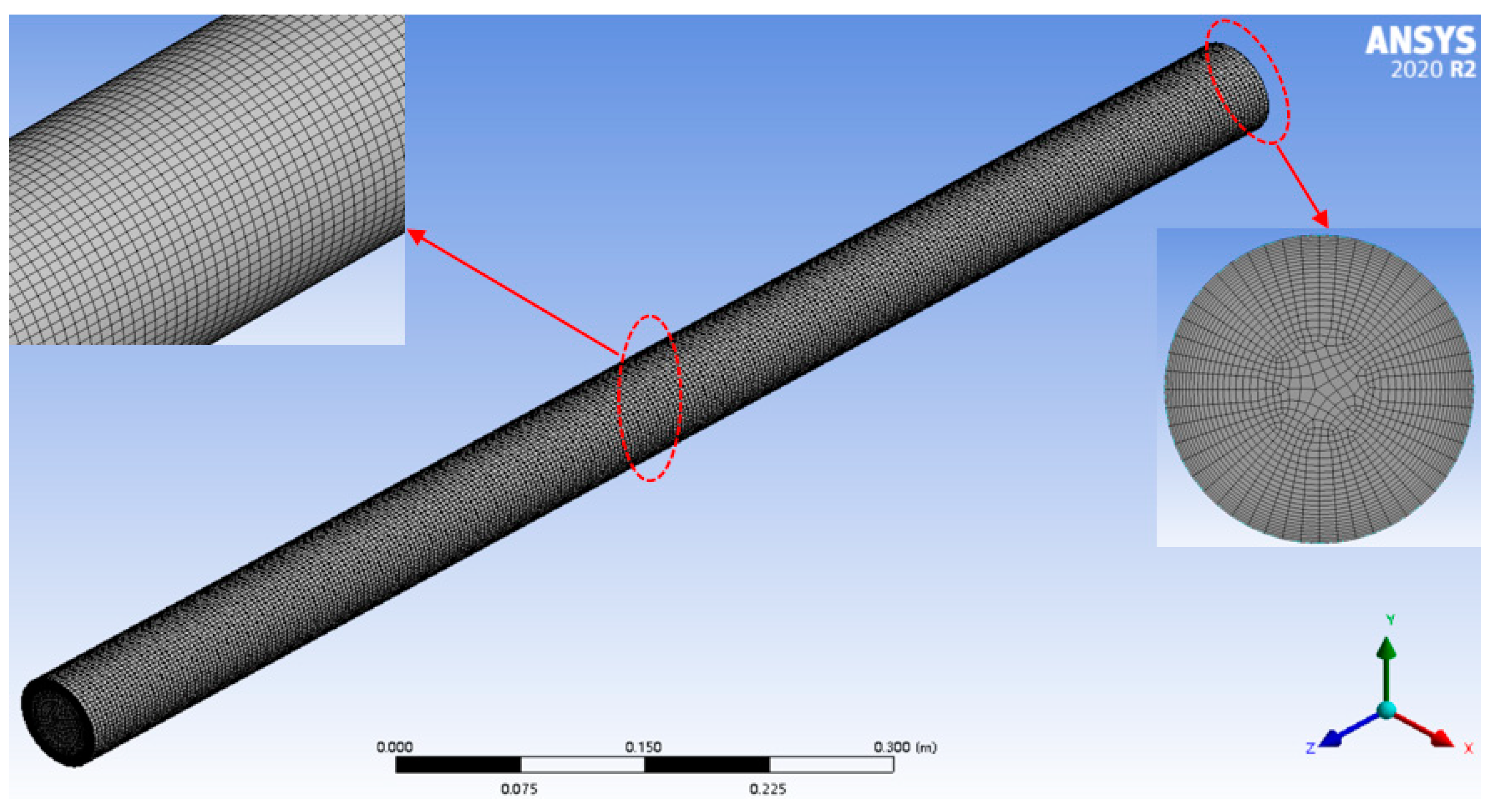
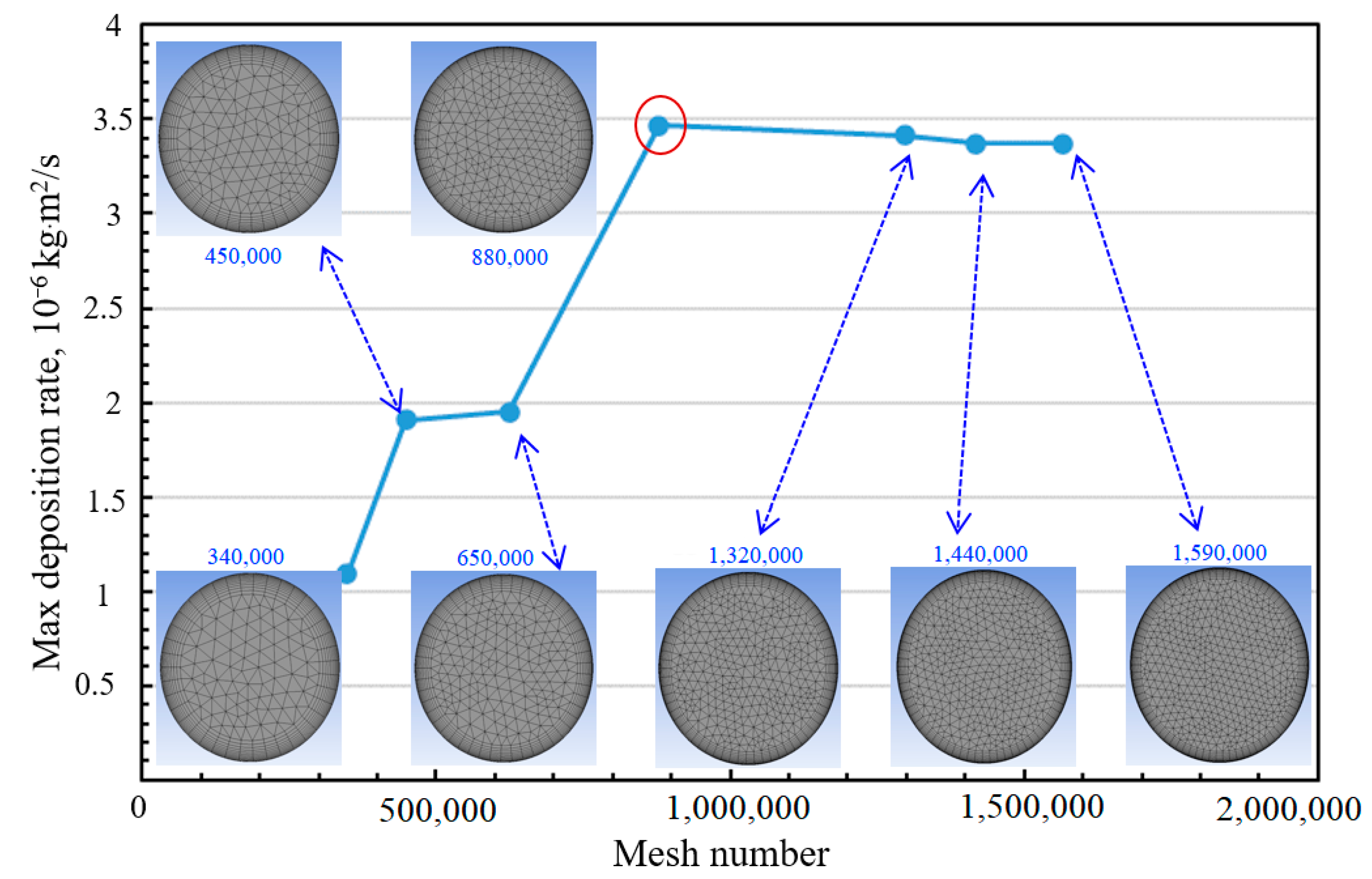
3.1. Geometry Generation and Mesh

In this study, a three-dimensional computational fluid dynamic simulation is used to investigate the deposition rate of asphaltene particles through the tube. In order to simulate the physics of the real-world blockage phenomenon, the inner diameter and length of the production tubing are set as 0.062 m and 1 m, respectively. Some details of the hexahedral mesh are shown in Figure 1. A smooth transitional inflation layer mesh is constructed as a result of the asphaltene deposition near the wall. The thickness of the first layer of the boundary layer is set to 0.5 mm, with a total of 20 layers, and the growth factor is 1.2. We use the grid-independent verification method, similarly to Gao [16], to determine the number of grids, and the final optimal number of grids is 7,420,652. The grid independence verification results are shown in Figure 2.

3.2. Boundary Condition

During the computational procedure, a range of gas–liquid superficial velocities are employed to induce various flow regimes in the tubing, including a bubbly flow, slug flow, agitated flow, and annular mist flow. The outlet is set as a pressure outlet, the turbulent flow intensity is set to 5%, and the turbulent flow diameter is equal to the pipe diameter, which is 0.062 m. In addition, the diameter distribution of the particles is Rosin–Rammler, particles of 10~400 μm are injected from the oil phase inlet, the particle velocity is equal to the oil flow velocity, and the particle density is 1100 kg/m³. The DPM of the entrance and exit is set to Escape, and the DPM of the wall is set to Trap. The simulation parameter settings are shown in

Table 2. Simulation parameter settings.

Parameter	Numerical Value
Diameter, m	0.62
Length, m	1
Crude oil density, m3/d	866
Inlet pressure, MPa	30
Outlet pressure, MPa	29.5
Asphaltene particle density, kg/m3	1100
Apparent velocity of liquid phase, m/s	0.5, 1, 2, 3, 4
Gas phase superficial velocity, m/s	1, 2, 3, 4, 5
Particle diameter, μm	50, 100, 200, 300, 400
Interfacial tension, n/m	0.02, 0.04, 0.06, 0.08, 0.1
Crude oil viscosity, mPa·s	0.012, 0.024, 0.036, 0.048, 0.06

.

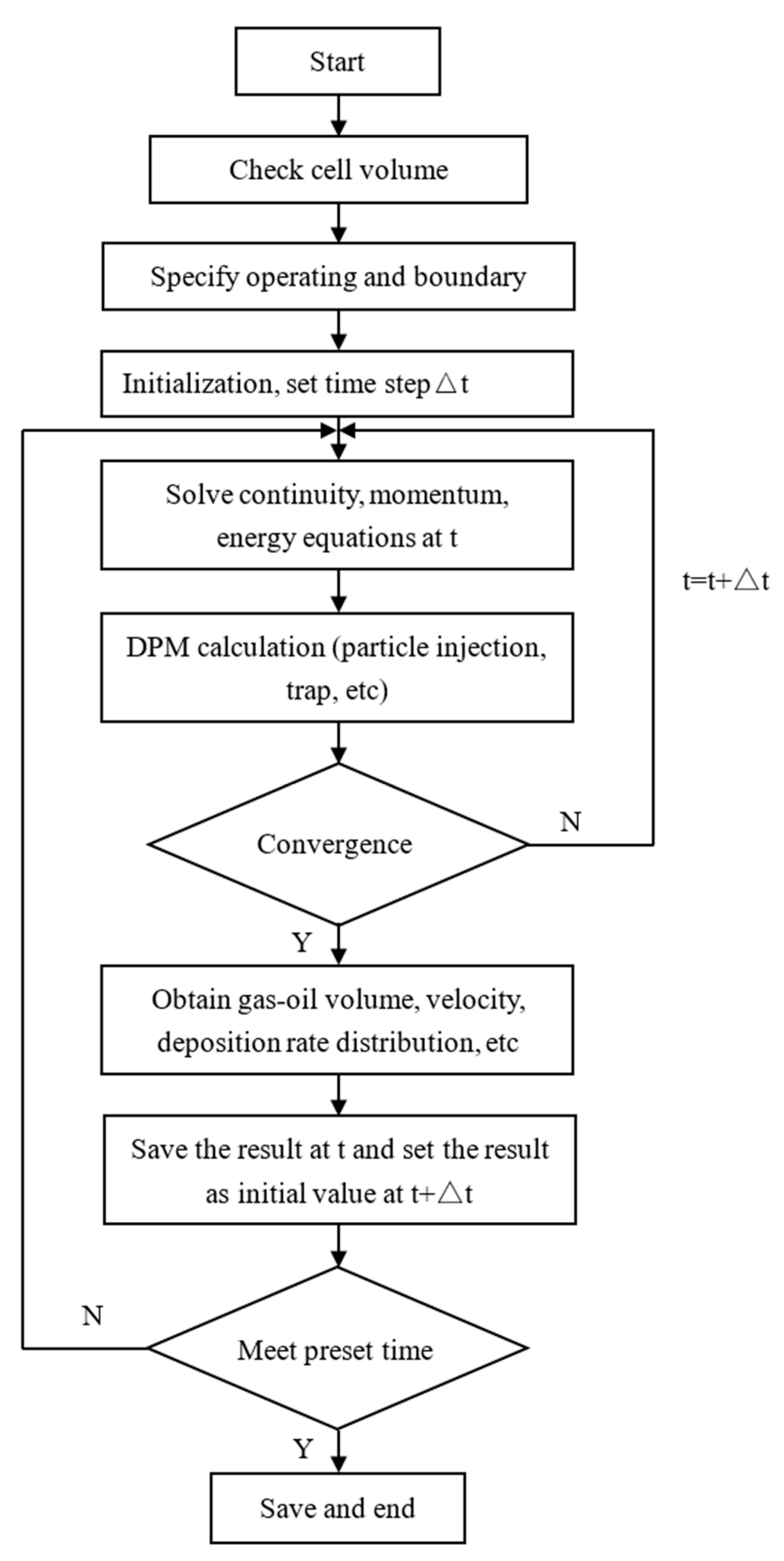
3.3. Calculation Method

The solution models generally include three types, SIMPLE, SIMPLEC, and PISO. The core idea of both the SIMPLEC and SIMPLE algorithms is to use the assumed pressure field to solve the momentum equation to obtain the flux on the boundary; the difference is that SIMPLEC corrects the flux to increase the convergence speed. The PISO algorithm adds momentum correction and grid distortion correction to the SIMPLE algorithm, which improves the accuracy and speed of the pressure field during transient simulation and greatly reduces the amount of CPU calculation. Therefore, this paper uses the PISO algorithm for transient simulation, uses Geo-Reconstruct for the volume fraction, and sets the Courant number to 0.25. In addition, during the simulation process, it is found that convergence difficulties occur when the time step is too large. In order to obtain a stable convergence solution, the pressure is set to 0.2, the density is set to 0.5, the time step is set to 0.001, and the maximum iteration step is 20 times. The time step is 1000 times. The transient simulation flow chart is shown in Figure 3.

4. CFD Simulation Results

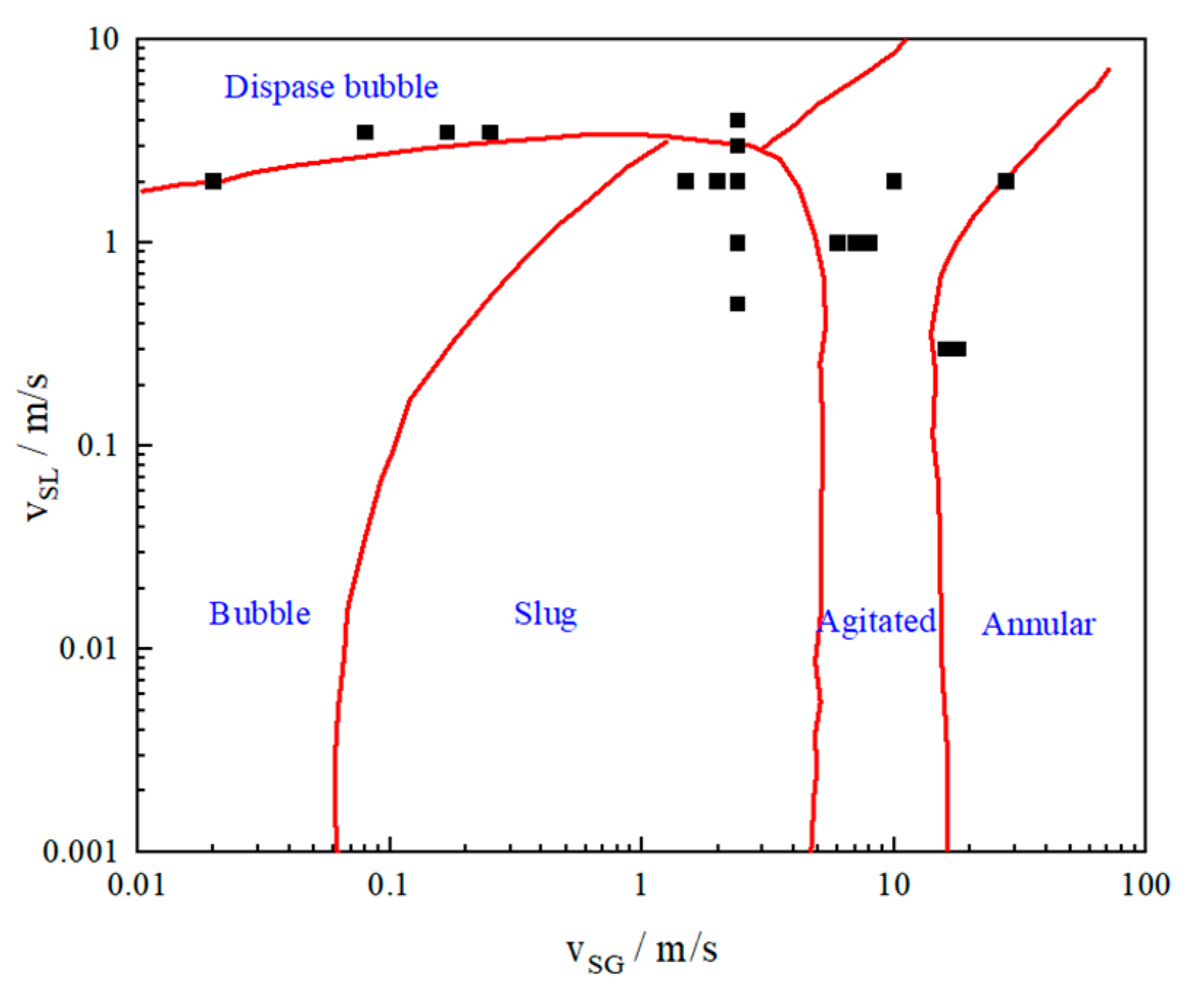
4.1. Model Validation for Gas–Oil Two Phases

Numerical simulation software (Fluent 2021.R1) was used to simulate the bubbly flow, slug flow, agitated flow, and annular fog flow in the vertical pipe, and the simulated gas–liquid phase distribution was compared with the schematic diagrams of the four flow patterns. During the simulation process, the gas phase and liquid phase superficial velocity used in this work are selected from the flow pattern obtained from the experimental research of Barnea et al. [36] (see Figure 4). In addition, according to the mass flow conservation, the production is assumed to be constant in the simulation process; since the bubble point pressure exceeds the multiphase flow, the liquid phase mass flow will decrease with the increase in the gas phase mass flow [37]. Considering the calculation cost, a total of 37 groups of gas–liquid two-phase flows are simulated in this paper, and the corresponding gas phase superficial velocities and liquid phase superficial velocities are marked in Figure 4.

4.1.1. Bubbly Flow

Figure 4 is the gas phase nephogram diagram in the axial (XZ) section and radial (XY) section of different gas phase superficial velocities in the bubbly flow. Due to the small volume fraction of bubbles in the tube during the bubbly flow, it is difficult to accurately distinguish whether there are bubbles, so the upper limit of the gas phase volume fraction is set to 0.7. The blue in the distribution diagram represents the oil phase volume fraction, the other colors represent the gas phase volume fraction, and the darker the color, the higher the gas content. It can be seen in Figure 5a that the bubbles are mainly distributed in the center of the pipe, and the pipe wall is dominated by the liquid phase. The gas phase volume fraction in the tubing and the superficial velocity increase correspondingly with the proportion. When the gas phase superficial velocity is set to 0.09 m/s, some bubbles are scattered in the XZ section, the gas phase volume distribution on the XZ interface increases significantly, and the volume fraction also increases accordingly as the velocity increases. When the speed increases to 0.25 m/s, it is found that the color of the gas phase cloud image on the XZ section is deepened, and the gas phase volume fraction in some positions is as large as 0.7; it is also observed that many small bubbles merge in the middle and upper parts of the tubing, making the volume larger. There are more bubble shapes, such as the hat shape, raindrop shape, inverted heart shape, etc.

Then, the gas–liquid phase distribution nephogram diagram at different heights and different gas phase superficial velocities of the tubing is analyzed, as shown in Figure 5b. It can be observed that the bubbles will coalesce with the increase in the gas phase superficial velocity at the same height, and the gas phase volume will increase accordingly. Generally speaking, the gas phase is the dispersed phase and the liquid phase is the continuous phase in the bubbly flow. 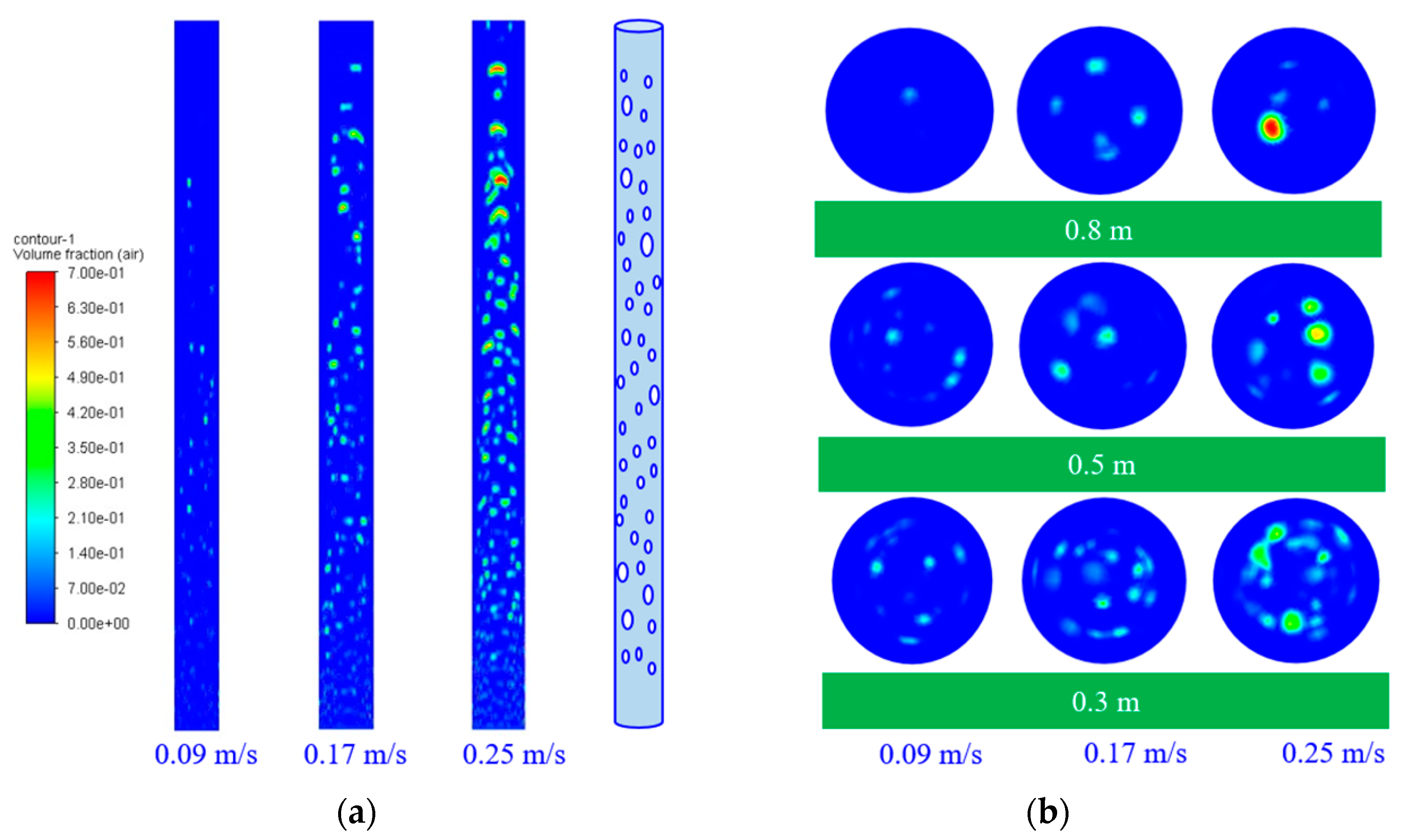In addition, comparing the simulated bubbly flow gas–liquid phase distribution nephogram with the schematic diagram, the bubble distribution structure is similar, indicating that the multiphase flow model can be used to simulate a bubbly flow.

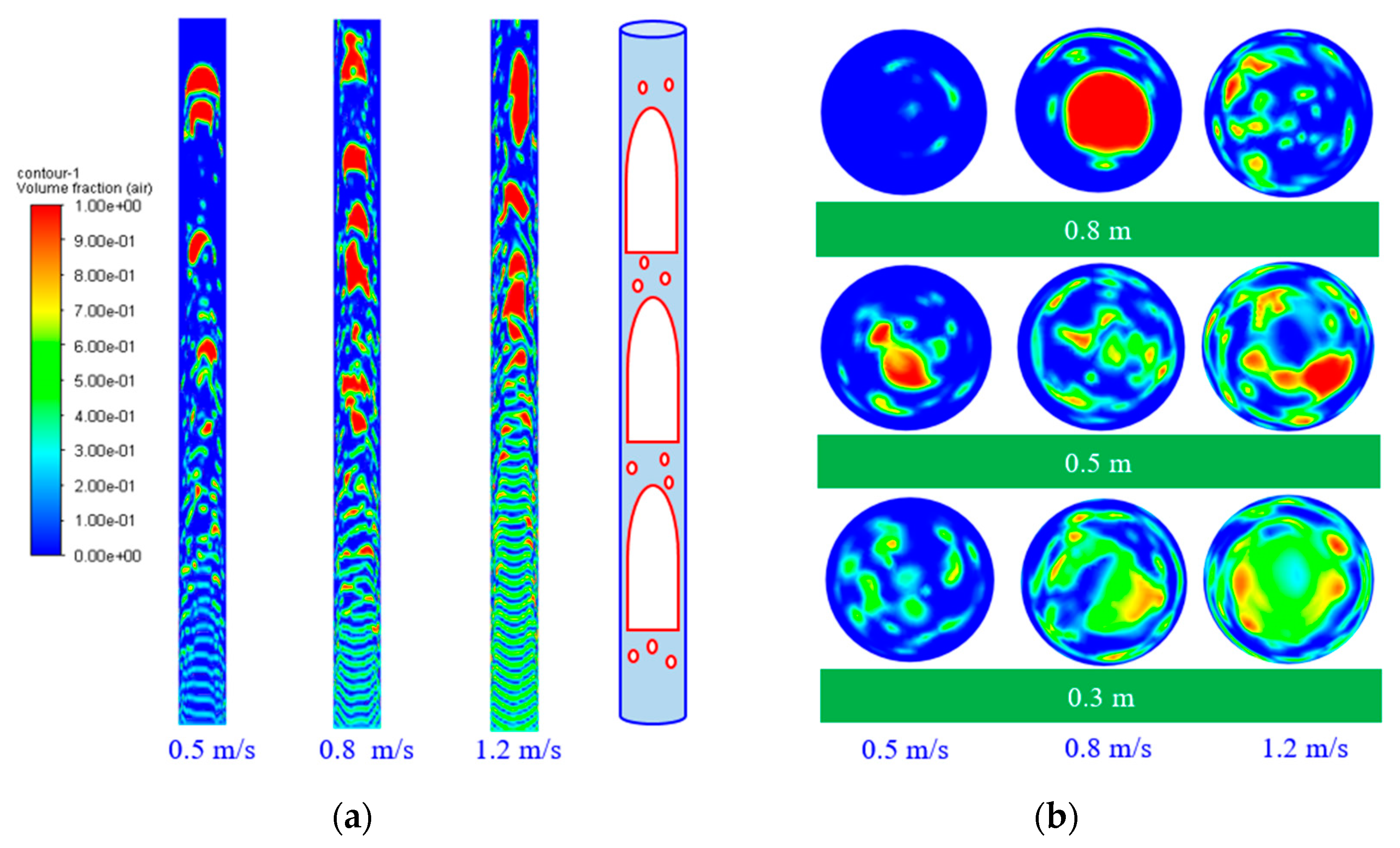
4.1.2. Slug Flow

As the superficial velocity of the gas phase increases, the flow pattern in the tube will change from a bubbly flow to a slug flow, with alternate rises of slugs and bubbles. It can be seen from the XZ axial section nephogram diagram in Figure 6a that the gas phase diagram in the slug flow tubing is richer in color, transitioning from blue and yellow to red, and the darker color indicates a higher gas phase volume fraction. In the slug flow, the tube wall is occupied by oil samples, and the volume distribution of the gas phase is more extensive than in the bubbly flow. Taking the nephogram image of the apparent velocity of the gas phase at 0.5 m/s as an example, it is found that the gas–liquid phase at the entrance enters in the form of a section of gas and a section of liquid.

The above phenomenon can also be observed from Figure 6b, which shows the XY section of the same gas phase superficial velocity. Comparing the gas–liquid phase distribution at different heights and superficial velocities, it is found that the volume distribution and gas phase fraction at the same height will increase with the increase in the gas superficial velocity. In addition, comparing the cloud diagram of the gas–liquid phase distribution of the slug flow with the schematic diagram, it is observed that the method is suitable for slug flow simulation.

4.1.3. Agitated Flow

It can be seen from the XZ axial cross-sectional cloud diagram in Figure 7a that the gas phase breaks through from the previous gas plug in the form of a gas column, almost occupying the entire section of the tubing. The oil phase also changes from the previous continuous phase to the dispersed phase.

The above phenomena are observed from the XY sections of the tubing at different heights and gas phase superficial velocities. It is found in Figure 7b that the liquid phase volume distribution and fraction will decrease with the increase in the gas superficial velocity at the same height (0.3 m, 0.5 m, and 0.8 m). This is because the intensity of the turbulent flow inside the tubing also increases with the gas superficial velocity. This strong turbulent kinetic energy scatters the liquid phase, and some small liquid droplets will be wrapped in the surrounding gas phase. 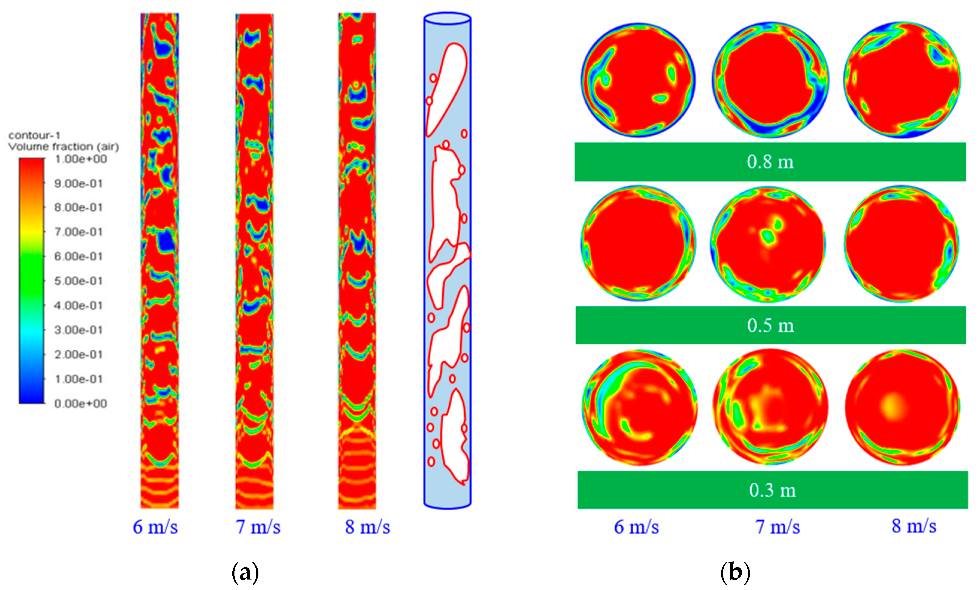In addition, the nephogram image of the gas–liquid phase distribution of the agitated flow is compared with the schematic diagram, which shows that the method can realize the simulation of the agitated flow.

4.1.4. Annular Flow

It can be seen from the XZ section in Figure 8a that the oil pipe is dominated by gas columns, whose diameter is almost equal to the inner diameter of the entire oil pipe, and some small droplets are scattered in the center of the gas column. The droplets are carried out of the wellhead by the velocity of the high-speed flowing gas phase. From the XY section in Figure 8b, it can be observed that a part of the liquid phase adheres to the tubing wall in the form of a thin oil ring. Comparing the cloud diagram and schematic diagram of the gas–liquid phase distribution of the annular fog flow, it is observed that the gas–liquid phase distribution structure is similar, indicating that it can be used to simulate the annular fog flow.

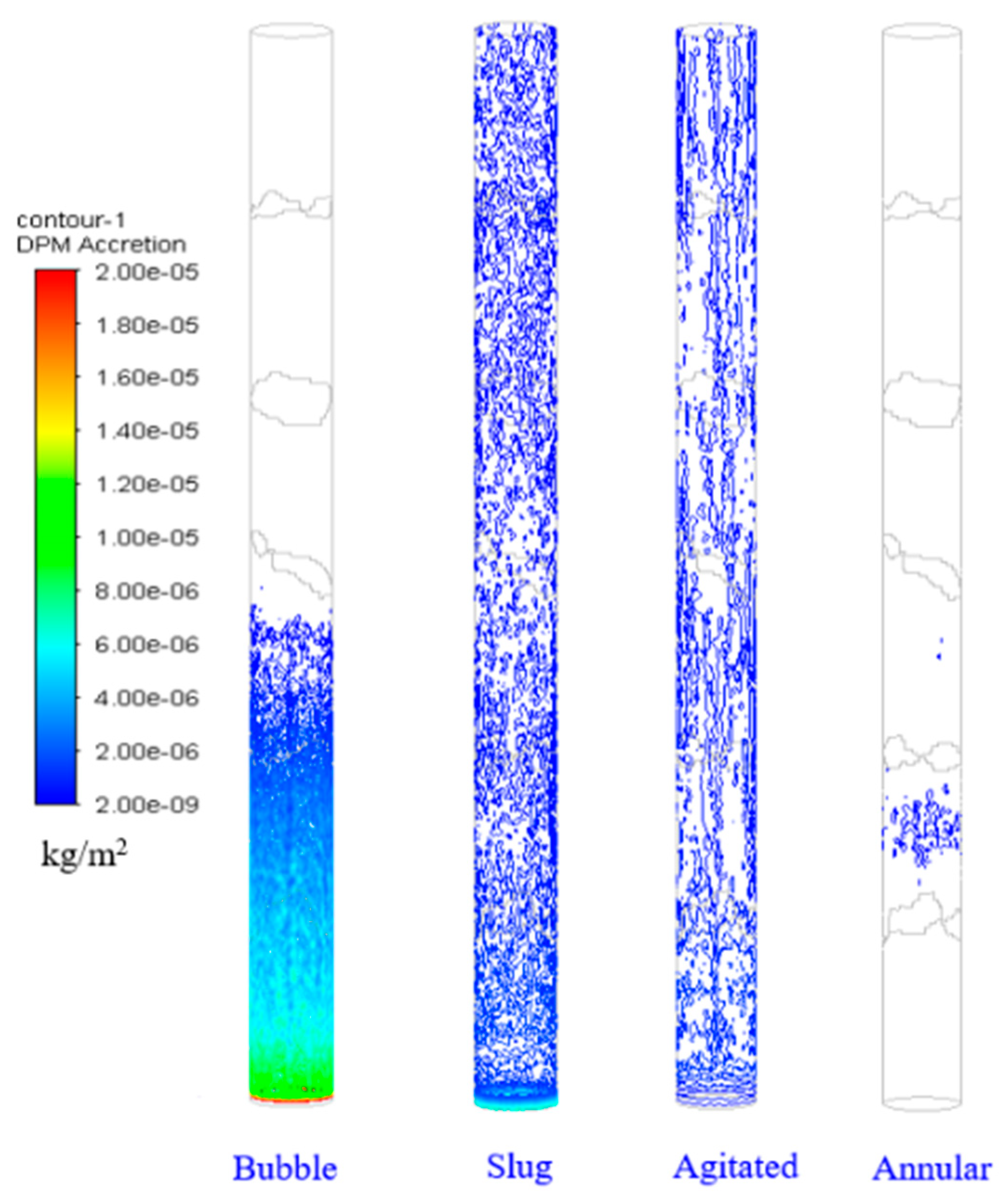
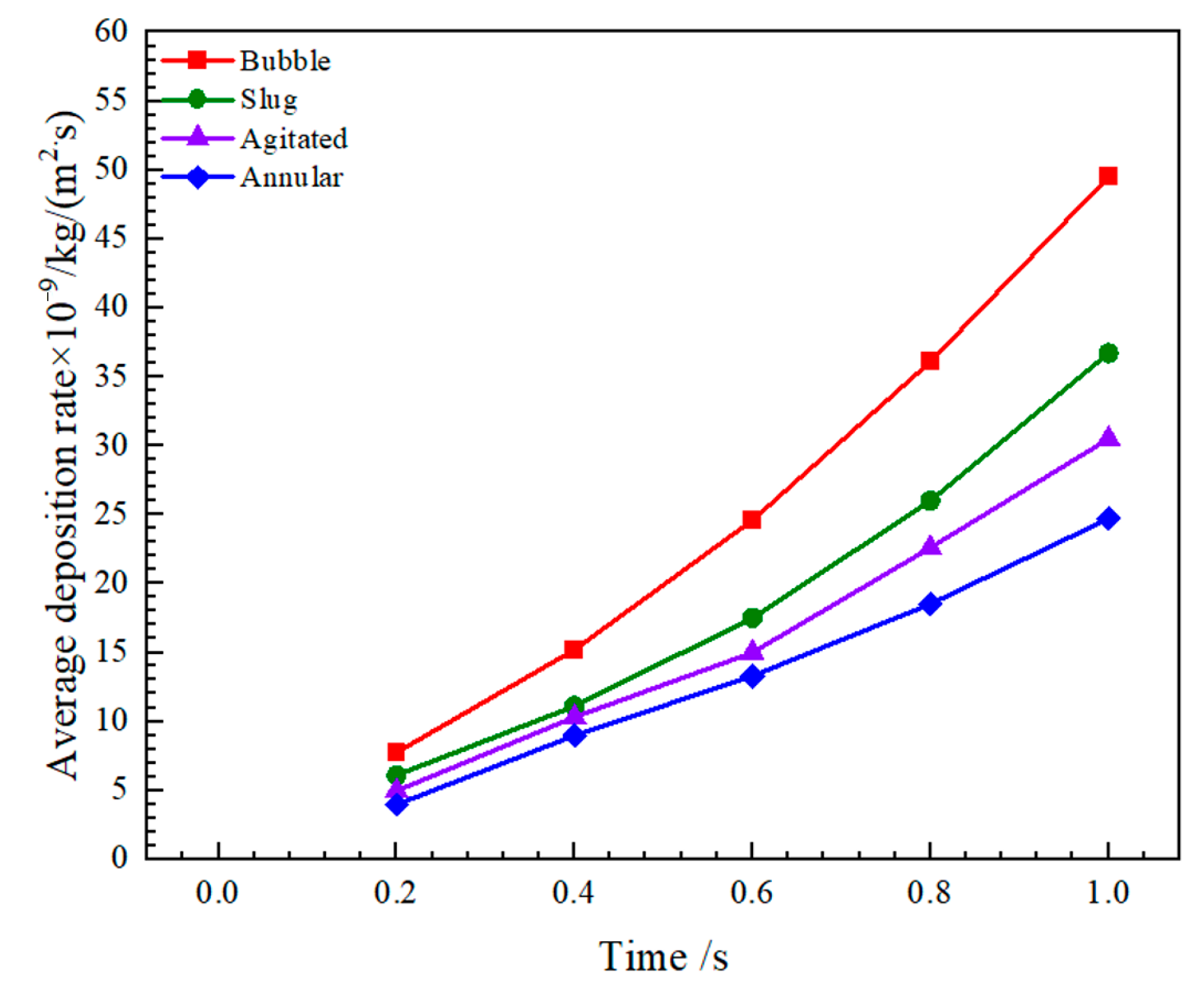
4.2. Comparison of Deposition Rates in Different Flow Patterns

The above simulation results show that the VOSET + standard k-ε turbulence model can be used to simulate the four flow patterns. On this basis, the DPM model is introduced; in this case, asphaltene particles are injected from the inlet end of the tubing, and the velocity of the asphaltene particles is consistent with the crude oil. Using the above simulation methods, the cloud diagrams of the deposition distribution of asphaltene particles in bubbly flow, slug flow, agitated flow, and ring fog flow are obtained, as shown in Figure 9.

It can be seen that the deposition of asphaltene in the pipe is mainly concentrated near the inlet section during bubbly flow, and the color of the deposition cloud is obviously better than that of the other three flow patterns. Asphaltene particles adhere to the entire pipe wall in the cases of slug flow and agitated flow, which also shows that as the flow velocity increases, the turbulent kinetic energy of the fluid in the pipe increases, which makes the adhesion increase. The annular flow distribution of the deposition volume is the lowest, which is mainly caused by an insufficient liquid volume. This point can also be observed from the cloud map of the gas–liquid phase distribution of the annular fog flow.

In order to quantitatively illustrate the relationship between the average deposition rate and the flow pattern, the influence of the flow pattern on the deposition rate at different times is analyzed, as shown in Figure 10. It can be seen that the average deposition rate of asphaltene particles in the bubbly flow is the largest (4.95 × 10⁻⁸ kg/(m²·s)), followed by the slug flow, agitated flow, and annular flow. This is because the oil phase volume and mass flow rate in the bubbly flow are relatively large, which will intensify the collision between particles and the pipe wall, thus increasing the deposition rate. In addition, compared with the other three flow patterns, the velocity of the mixed fluid in the bubbly flow is lower, and the slow flow in the tube will increase the probability of particle adhesion on the tube wall, which will also increase the deposition rate. The flow state in the tubing will transition from bubbly to annular flow as the gas phase velocity increases. According to mass conservation, the mass flow rate of the liquid phase in the oil pipe will decrease due to the increase in the gas phase flow rate, so that the precipitated asphaltene particles in the oil phase will decrease. Although the increase in the gas phase velocity will increase the mixing velocity and turbulence intensity in the tubing, the average deposition rate of asphaltene in the other flow patterns is obviously lower than that in the bubbly flow.

4.3. Sensitivity Analysis

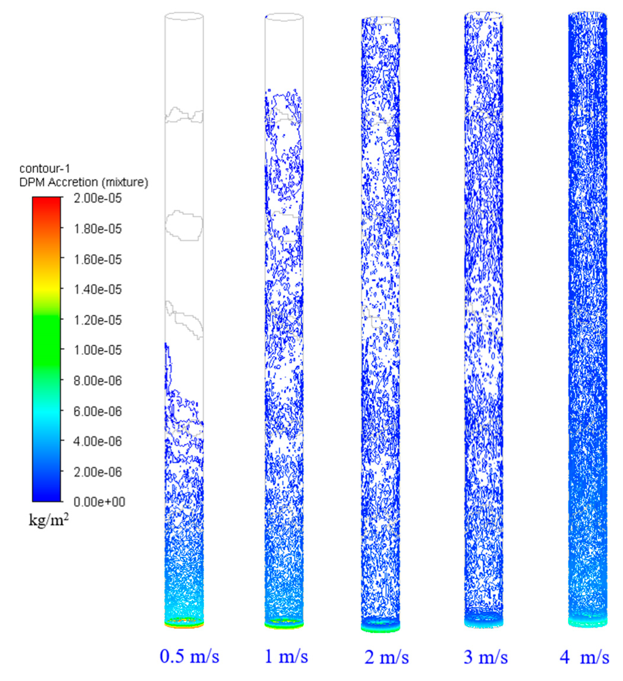
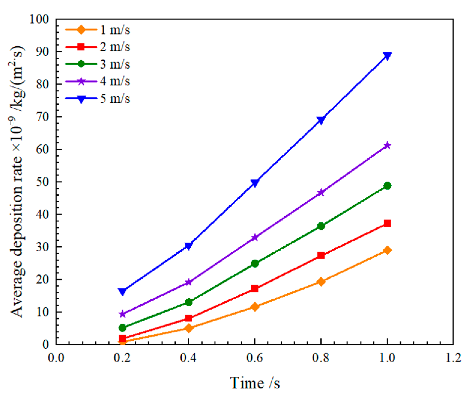
4.3.1. Effect of Gas Superficial Velocity on Deposition Rate

In order to clarify the effect of the gas superficial velocity on the asphaltene deposition rate, the liquid phase superficial velocity is simulated at 2 m/s, and the gas phase velocity is 0.5 m/s, 1 m/s, 2 m/s, 3 m/s, and 4 m/s, respectively.

It can be seen from Figure 11 that the color and distribution of the asphaltene deposition clouds on the tubing wall gradually increase as the superficial velocity of the gas phase increases. In order to more accurately describe the influence of different gas phase superficial velocities on the average deposition rate, the results are quantified (see Figure 12). It can be observed that the average deposition rate is 2.27 × 10⁻⁸ kg/(m²·s) when the gas phase superficial velocity is 0.5 m/s. The average deposition rate increases by 82% when the gas superficial velocity increases by 4 m/s. This is because the mass flow rate of the asphaltene particles precipitated in the crude oil remains constant, and the turbulent kinetic energy of the mixed fluid inside the tubing becomes stronger as the superficial velocity of the gas phase increases. This state will intensity the asphaltene particle–particle and particle–wall collisions and thus increase the probability of adhesion, in line with the deposition rate.

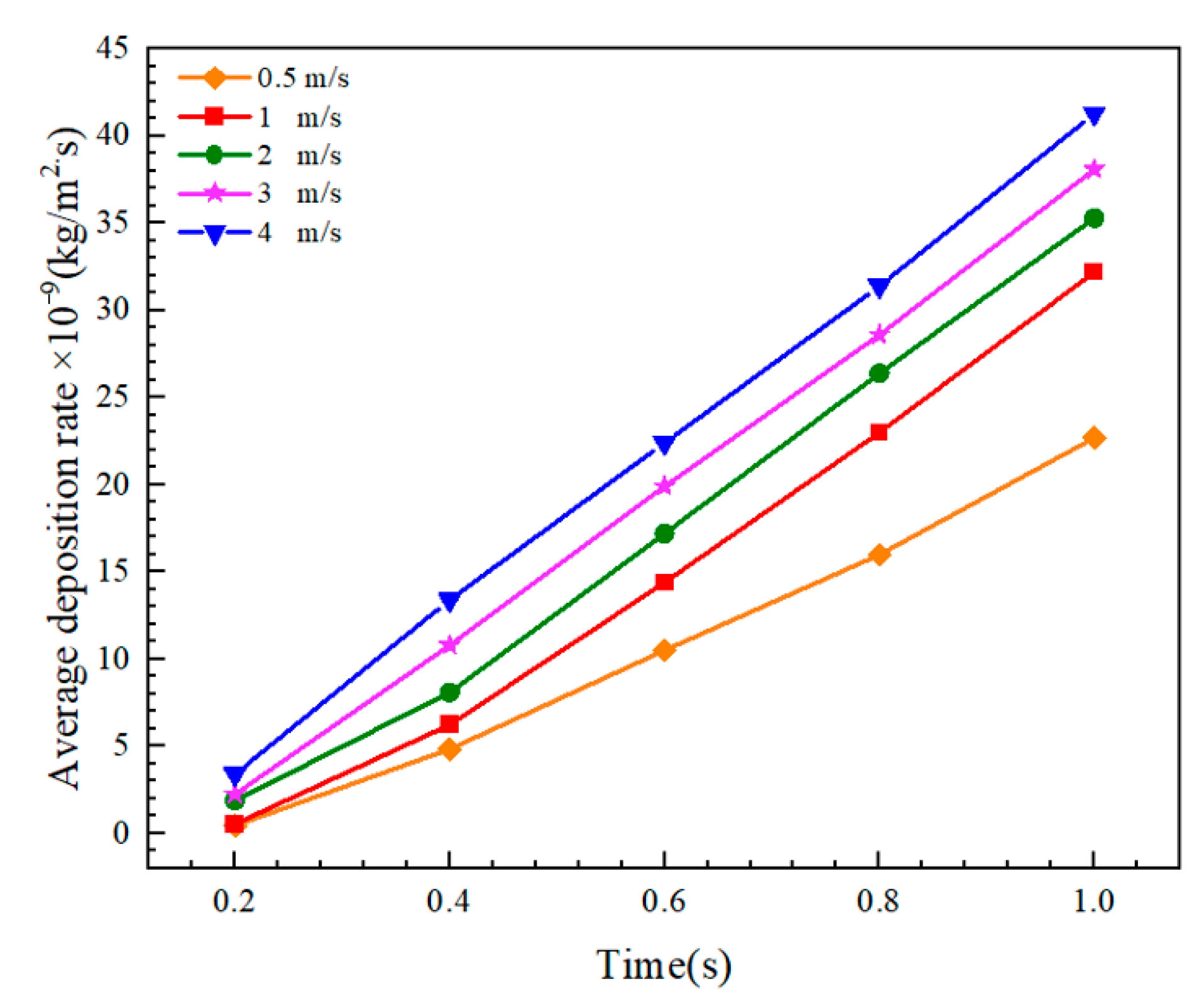
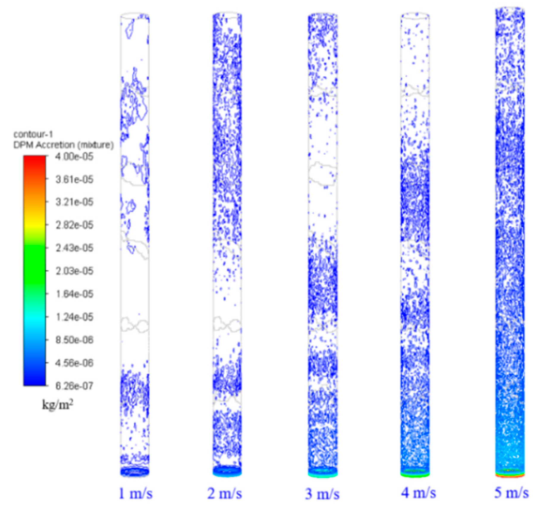
4.3.2. Effect of Liquid Superficial Velocity on Deposition Rate

The asphaltene deposition distribution in the tubing was calculated when the superficial velocity of the gas phase was 2 m/s and the superficial velocity of the liquid phase was 1 m/s, 2 m/s, 3 m/s, 4 m/s, and 5 m/s, as shown in Figure 13.

It can be observed that the distribution area of the asphaltene deposition cloud map on the pipe wall increases as the superficial velocity of the liquid phase increases. The color becomes darker, indicating that the amount of asphaltene deposition increases accordingly. In order to quantitatively illustrate the relationship between the average deposition rate and the superficial velocity of the liquid phase, the influence of the liquid phase superficial velocity is displayed in Figure 14. It can be seen that the average deposition rate of asphaltene is approximately 2.9 × 10⁻⁸ kg/(m²·s) at 1 m/s. The deposition rate of the asphaltene particles will increase as the superficial velocity of the liquid phase increases. The average deposition rate increased by 2.1 times at 5 m/s, since the mass flow rate of asphaltene particles increases significantly with the increase in the liquid phase mass flow rate, and a higher particle mass flow rate will increase the probability of adhesion, which will lead to a corresponding increase in the deposition rate.

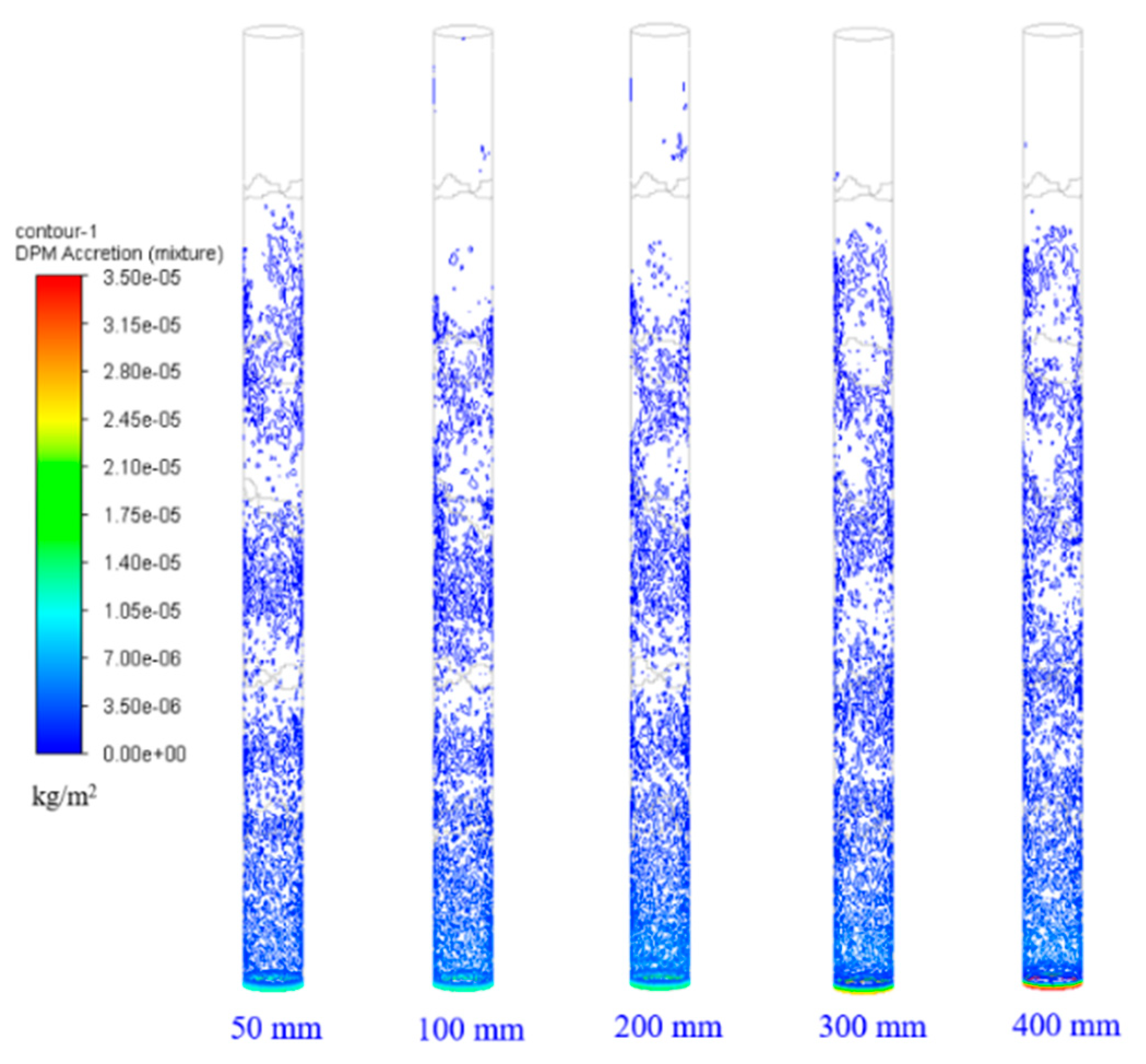
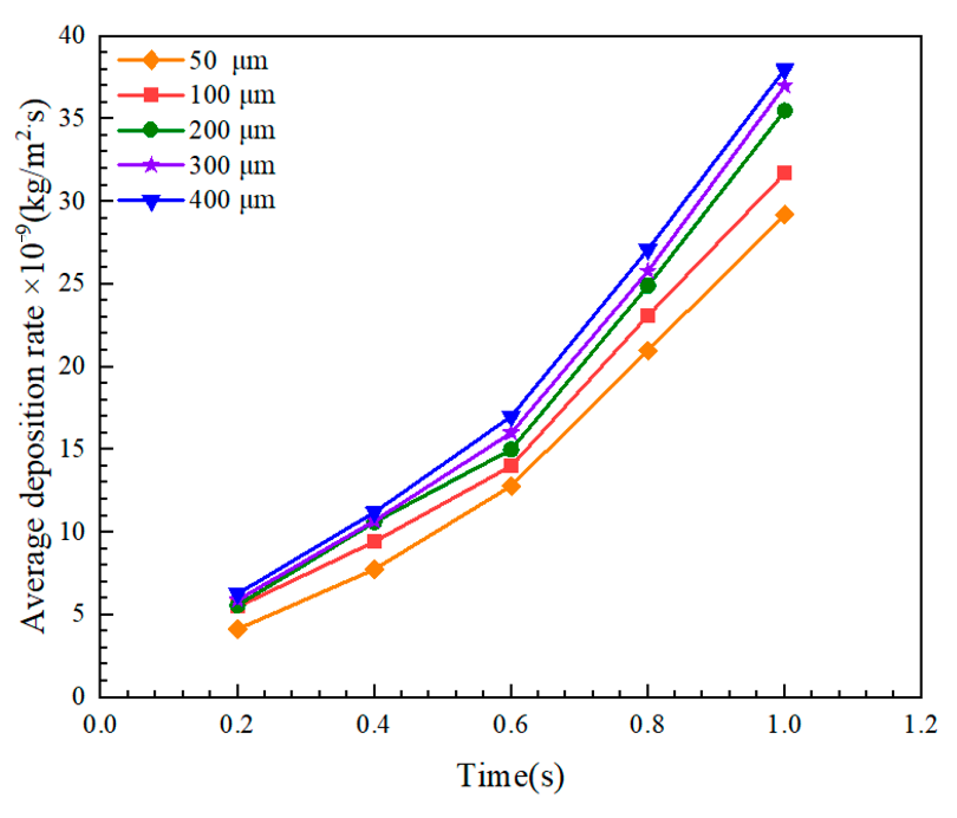
4.3.3. Effect of Particle Diameter on Deposition Rate

The deposition distribution of asphaltene particles in the tubing was calculated when the gas phase superficial velocity was 1 m/s, the liquid phase superficial velocity was 2 m/s, and the particle diameters were 50 μm, 100 μm, 200 μm, 300 μm, and 400 μm, respectively, as shown in Figure 15.

It can be seen that the distribution of asphaltene deposition in oil pipes with five different particle diameters is almost the same; the difference is that the color of the asphaltene deposition cloud image at the inlet end deepens with the increase in particle diameter. The average deposition rate of asphaltene at 50 μm was 2.92 × 10⁻⁸ kg/(m²·s), as seen in Figure 16, and it increased by 27% when the particle size increased to 400 μm. This is because the high inertial and Saffman lift forces of the particles lead to a higher deposition rate.

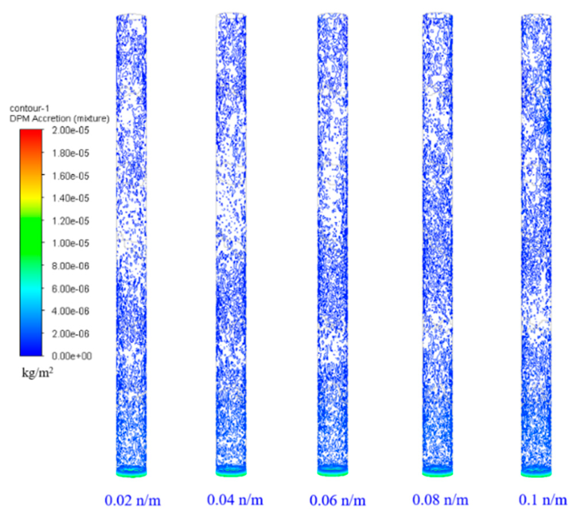
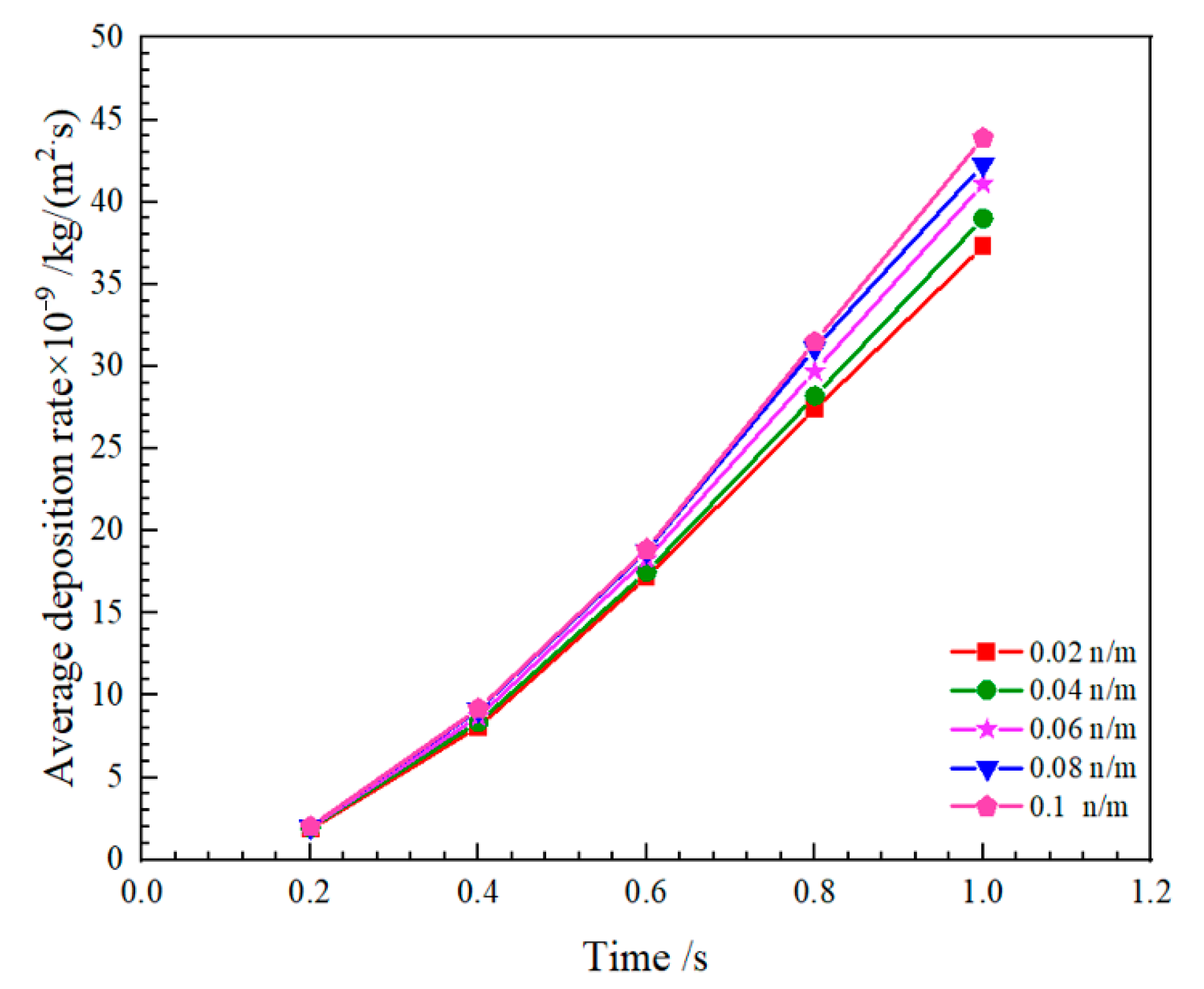
4.3.4. Effect of Interfacial Tension on Deposition Rate

Oil–gas interfacial tension reflects the strength of the force of oil–gas molecules. Changes in the crude oil composition, temperature, and pressure will cause changes in interfacial tension. It is calculated that the superficial velocity of the gas phase is 1 m/s, the superficial velocity of the liquid phase is 2 m/s, and the interfacial tension of oil and gas is 0.02 n/m, 0.04 n/m, 0.06 n/m, 0.08 n/m, and 0.1 n/m, respectively. The distribution of the asphaltene deposits in the tubing is shown in Figure 17.

It can be seen from Figure 17 that the color of the deposition cloud image and the distribution of the deposition amount corresponding to the five oil–gas interfacial tensions have little change, which means that the deposition rates corresponding to the five interfacial tensions are relatively close. In order to accurately analyze the influence of interfacial tension on the average deposition rate, the cloud images of the deposition rate distribution obtained at different times were quantitatively processed, as shown in Figure 18. It can be seen that the average deposition rate increases by 18% from 0.02 n/m to 0.1 n/m. The reason is that the surface tension in VOF actually balances the radially inward attraction between molecules and the radially outward pressure gradient force on the molecular surface. The higher the surface tension, the larger the bubbles and the more difficult it is to achieve a force balance. In addition, according to Formula (6), it can be seen that the momentum will increase with the increase in the surface tension, so the average deposition rate will increase.

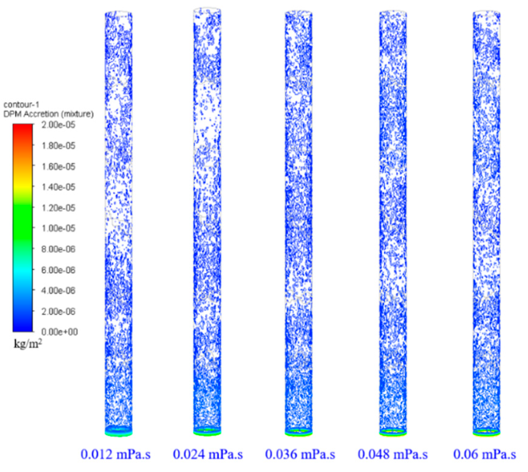
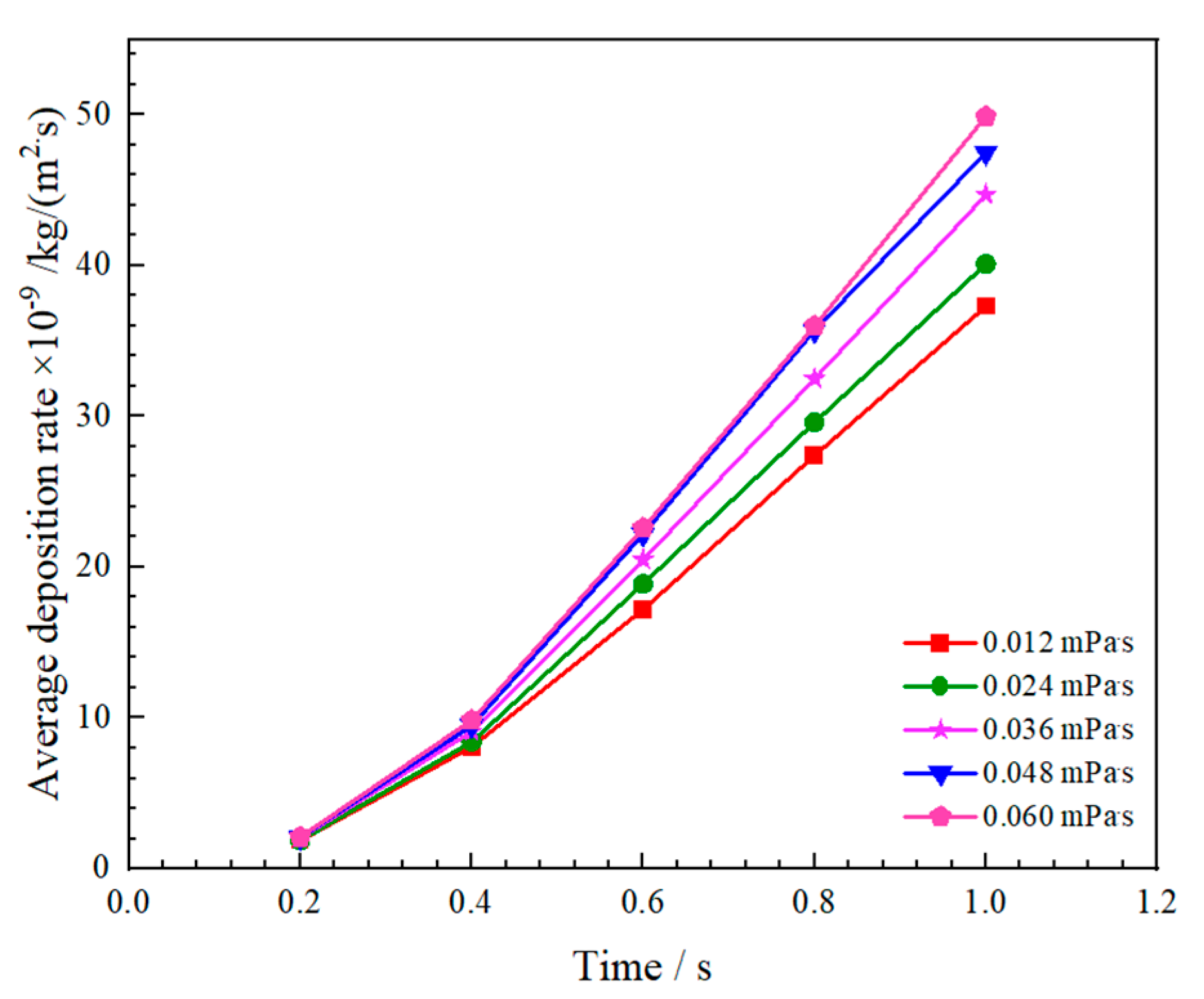
4.3.5. Effect of Oil Viscosity on Deposition Rate

The viscosity determines the difficulty of crude oil flow. In order to study the influence of the crude oil viscosity on the average deposition rate of asphaltene, the gas phase superficial velocity is calculated as 2 m/s, the liquid phase superficial velocity is 2 m/s, and the crude oil viscosity is 0.012 mPa·s, 0.024 mPa·s, 0.036 mPa·s, 0.048 mPa·s, and 0.06 mPa·s, as shown in Figure 19.

It can be seen that the color changes of the five types of sedimentary cloud maps are small, indicating that their deposition rates are not much different. In order to quantitatively analyze them, the relationship between the viscosity of crude oil and the deposition rate is displayed. To precisely assess the impact of the crude oil viscosity on the average deposition rate, cloud images depicting the distribution of the deposition rates, captured at various time points, were subjected to quantitative analysis, as illustrated in Figure 20. It is found that the viscosity of crude oil increases from 0.012 mPa·s to 0.06 mPa·s, and the average deposition rate increases by 34%. This is because the viscosity of crude oil increases exponentially with the content of asphaltene, and an increase in asphaltene content will increase the frequency of particles colliding on the pipe wall, thus causing the high average deposition rate.

5. Conclusions

This work mainly studies the deposition of asphaltene particles on the tubing wall in a multiphase flow. The VOSET + k-ε turbulence model was used to simulate the two-phase flow of oil and gas in the tubing, and the DPM model was used to inject asphaltene particles into the tubing. In addition, the effects of the gas phase superficial velocity, liquid phase superficial velocity, particle diameter, oil–gas interfacial tension, and crude oil viscosity on the asphaltene deposition rate were analyzed. The main conclusions are as follows.

(1)

The deposition rates of asphaltene particles in the four flow patterns are observed to follow the order of bubble flow > slug flow > agitated flow > annular mist flow.

(2)

The deposition rate is observed to be the highest in bubble flow, while it is the lowest in annular flow. Specifically, the deposition rates in bubble flow are 1.35, 1.62, and 2 times greater than those in slug flow, churning flow, and annular mist flow, respectively.

(3)

The average deposition rate of asphaltene is escalated with a rise in the gas phase superficial velocity, liquid phase superficial velocity, particle size, oil–gas interfacial tension, and crude oil viscosity. The gas phase apparent velocity, particle diameter, and interfacial tension increase the deposition rate through changes in fluid kinetic energy. Conversely, the liquid phase apparent velocity and crude oil viscosity contribute to an increase in the deposition rate by amplifying the asphaltene content.

References

- Tavakkoli, M.; Panuganti, S.R.; Taghikhani, V.; Pishvaie, M.R.; Chapman, W.G. Understanding the polydisperse behavior of asphaltenes during precipitation. Fuel 2014, 117, 206–217. [Google Scholar] [CrossRef]
- Kokal, S.L.; Sayegh, S.G. Asphaltenes: The cholesterol of petroleum. In Middle East Oil Show; Society of Petroleum Engineers: Tulsa, OK, USA, 1995; Available online: https://www.onepetro.org/conference-paper/SPE-29787-MS (accessed on 25 November 2023).
- Decanio, S.J.; Nero, V.P.; DeTar, M.M.; Storm, D.A. Determination of the molecular weights of the Ratawi vacuum residue fractions- a comparison of mass spectrometric and vapour phase osmometry techniques. Fuel 1990, 69, 1233–1236. [Google Scholar] [CrossRef]
- Ancheyta, J.; Centeno, G.; Trejo, F.; Marroquín, G.; García, J.A.; Tenorio, E.; Torres, A. Extraction and characterization of asphaltenes from different crude oils and solvents. Energy Fuels 2002, 16, 1121–1127. [Google Scholar] [CrossRef]
- Sato, S.; Takanohashi, T.; Tanaka, R. Molecular weight calibration of asphaltenes using gel permeation chromatography/mass spectrometry. Energy Fuels 2005, 19, 1991–1994. [Google Scholar] [CrossRef]
- Amiri, R.; Khamehchi, E.; Ghaffarzadeh, M.; Kardani, N. Static and dynamic evaluation of a novel solution path on asphaltene deposition and drag reduction in flowlines: An experimental study. J. Pet. Sci. Eng. 2021, 205, 108833. [Google Scholar] [CrossRef]
- Zhang, J.; Tian, Y.; Qiao, Y.; Yang, C.; Shan, H. Structure and Reactivity of Iranian Vacuum Residue and Its Eight Group-Fractions. Energy Fuels 2017, 31, 8072–8086. [Google Scholar] [CrossRef]
- Schucker, R.; Kewwshan, R. Reactivity of Cold Lake asphaltenes. Am. Chem. Soc. Div. Fuel Chem. 1980, 25, 327–346. [Google Scholar]
- Ibrahim, H.H.; Idem, O.R. Interrelationships between asphaltene precipitation inhibitor effectiveness, asphaltenes characteristics, and precipitation behavior during n-heptane (light paraffin hydrocarbon)-induced asphaltene precipitation. Energy Fuels 2004, 18, 1038–1048. [Google Scholar] [CrossRef]
- Chen, C.; Guo, J.; An, N.; Pan, Y.; Li, Y.; Jiang, Q. Study of asphaltene dispersion and removal for high-asphaltene oil wells. Pet. Sci. 2021, 9, 551–557. [Google Scholar] [CrossRef]
- Thomas, F.; Bennion, D.; Hunter, B. Experimental and theoretical studies of solids precipitation from reservoir fluid. J. Can. Petrol. Technol. 1992, 31, 11. [Google Scholar] [CrossRef]
- Hammami, A.; Phelps, C.H.; Monger-McClure, T.; Little, T.M. Asphaltene precipitation from live oils: An experimental investigation of onset conditions and reversibility. Energy Fuels 2000, 14, 14–18. [Google Scholar] [CrossRef]
- Andersen, S.I. Effect of precipitation temperature on the composition of n-heptane asphaltenes. Fuel Sci. Technol. Int. 1994, 12, 51–74. [Google Scholar] [CrossRef]
- Haskett, C.E.; Tartera, M. A Practical Solution to the Problem of Asphaltene Deposits Hassi Messaoud Field, Algeria. J. Pet. Technol. 1965, 17, 387–391. [Google Scholar] [CrossRef]
- Alkafeef, S.F.; Al-Medhadi, F.; Al-Shammari, A.D. A Simplified Method to Predict and Prevent Asphaltene Deposition in Oilwell Tubings: Field Case. SPE Prod. Oper. 2005, 20, 126–132. [Google Scholar] [CrossRef]
- Creek, J.L. Freedom of Action in the State of Asphaltenes: Escape from Conventional Wisdom. Energy Fuels 2005, 19, 1212–1224. [Google Scholar] [CrossRef]
- Vargas, F.M. Modeling of Asphaltene Precipitation and Arterial Deposition; Rice University: Houston, TX, USA, 2009. [Google Scholar]
- Gao, X.; Dong, P.; Chen, X.; Nkok, L.Y.; Zhang, S.; Yuan, Y. CFD modeling of virtual mass force and pressure gradient force on deposition rate of asphaltene aggregates in oil wells. Pet. Sci. Technol. 2022, 40, 995–1017. [Google Scholar] [CrossRef]
- Broseta, D.; Robin, M.; Savvidis, T.; Fejean, C.; Durandeau, M.; Zhou, H. Detection of asphaltene deposition by capillary flow measurements. In SPE/DOE Improved Oil Recovery Symposium; Society of Petroleum Engineer: Tulsa, OK, USA, 2000. [Google Scholar]
- Ekholm, P.; Blomberg, E.; Claesson, P.; Auflem, I.H.; Sjöblom, J.; Kornfeldt, A. A quartz crystal microbalance study of the adsorption of asphaltenes and resins onto a hydrophilic surface. J. Colloid Interface Sci. 2002, 247, 342–350. [Google Scholar] [CrossRef]
- Zougari, M.; Hammami, A.; Broze, G.; Fuex, N. Live oils novel organic solid deposition and control device: Wax and asphaltene deposition validation. In SPE Middle East Oil and Gas Show and Conference; Society of Petroleum Engineers: Tulsa, OK, USA, 2005. [Google Scholar]
- Vilas Bôas Fávero, C.; Hanpan, A.; Phichphimok, P.; Binabdullah, K.; Fogler, H.S. Mechanistic investigation of asphaltene deposition. Energy Fuels 2016, 30, 8915–8921. [Google Scholar] [CrossRef]
- Zhu, H.; Jing, J.; Chen, J.; Li, Q.; Yu, X. Simulations of deposition rate of asphaltene and flow properties of oil-gas-water three-phase flow in submarine pipelines by CFD. In Proceedings of the IEEE International Conference on Computer Science & Information Technology, Chengdu, China, 9–11 July 2010. [Google Scholar]
- Haghshenasfard, M.; Hooman, K. CFD modeling of asphaltene deposition rate from crude oil. J. Pet. Sci. Eng. 2015, 128, 24–32. [Google Scholar] [CrossRef]
- Seyyedbagheri, H.; Mirzayi, B. CFD modeling of high inertia asphaltene aggregates deposition in 3D turbulent oil production wells. J. Pet. Sci. Eng. 2017, 150, 257–264. [Google Scholar] [CrossRef]
- Emani, S.; Shaari, R. Discrete phase-CFD simulations of asphaltenes particles deposition from crude oil in shell and tube heat exchangers. Appl. Therm. Eng. 2019, 149, 105–118. [Google Scholar] [CrossRef]
- Martyushev, D.A. Modeling and prediction of asphaltene-resin-paraffinic substances deposits in oil production wells. Georesursy 2020, 22, 86–92. [Google Scholar] [CrossRef]
- Syuzev, A.V.; Lekomtsev, A.V.; Martyushev, D.A. Complex method of selecting reagents to delete asphaltenosmolaparinine deposits in mechanized oil-producing wells. Bull. Tomsk. Polytech. Univ. Geo Assets Eng. 2018, 329, 15–24. [Google Scholar]
- Parsi, M.; Agrawal, M.; Srinivasan, V.; Vieira, R.E.; Torres, C.F.; McLaury, B.S.; Shirazi, S.A. CFD simulation of sand particle erosion in gas-dominant multiphase flow. J. Nat. Gas Sci. Eng. 2015, 27, 706–718. [Google Scholar] [CrossRef]
- Parsi, M.; Kara, M.; Agrawal, M.; Kesana, N.; Jatale, A.; Sharma, P.; Shirazi, S. CFD simulation of sand particle erosion under multiphase flow conditions. Wear 2017, 15, 1176–1184. [Google Scholar] [CrossRef]
- Rao, Y.; Liu, Z.; Wang, S.; Li, L. Numerical Simulation on the Flow Pattern of a Gas-Liquid Two-Phase Swirl Flow. ACS Omega 2022, 7, 2679–2689. [Google Scholar] [CrossRef] [PubMed]
- Cerne, G.; Petelin, S.; Tiselj, I. Coupling of the interface tracking and the two-fluid models for the simulation of incompressible two-phase flow. J. Comput. Phys. 2001, 171, 776–804. [Google Scholar] [CrossRef]
- Elghobashi, S. Particle-laden turbulent flows: Direct simulation and closure models. Appl. Sci. Res. 1991, 48, 301–314. [Google Scholar] [CrossRef]
- Haider, A.; Levenspiel, O. Drag Coefficient and Terminal Velocity of Spherical and Nonspherical Particles. Powder Technol. 1989, 58, 63–70. [Google Scholar] [CrossRef]
- PSaffman, G. The lift on a small sphere in a slow shear flow. J. Fluid Mech. 1965, 22, 385–400. [Google Scholar] [CrossRef]
- Barnea, D. A unified model for predicting flow-pattern transitions for the whole range of pipe inclinations. Int. J. Multiph. Flow 1987, 13, 1–12. [Google Scholar] [CrossRef]
- Alhosano, A.; Daraboina, N. Effect of multi-phase flow on asphaltene deposition: Field case application of integrated simulator. J. Pet. Sci. Eng. 2021, 206, 1–14. [Google Scholar] [CrossRef]