A Method for Matching Unconventional Wells and Reservoirs Based on Semi-Analytic Models

Abstract

Unconventional well technology is often used as one of the most important means to reduce costs and increase efficiency in oil fields. There are many methods for unconventional well type optimization, but there are relatively few studies on whether the well type is suitable for the reservoir. In this paper, a method for matching unconventional wells and reservoirs is established. In our method, we first simplify the reservoir and choose initial suitable well types based on experience and then use a semi-analytical model to calculate the production rate in different producing sections. After that, we define some parameters to evaluate the matching degree of well types and reservoirs. Finally, we determine whether these well types are suitable for the reservoir based on these parameters. At the end of the paper, we apply the method to a specific case. The result shows that a stepped well is suitable for exploiting thin interbed reservoirs, but it is necessary that the permeability and fluid viscosity in different layers are within a certain range, and the shape of the stepped well is also limited. This paper gives a specific value for this range and limitation. The method for matching unconventional wells and reservoirs proposed in this paper is helpful for guiding the selection of unconventional well types before drilling.

1. Introduction

Unconventional wells refer to all wells with complex structure or process features, excluding vertical wells and including horizontal wells, stepped wells, multilateral wells, and other types of wells [1]. With the current maturity of drilling technology [2,3,4,5,6], unconventional wells account for more than half of the total number of wells drilled worldwide at present [7], and the use of unconventional wells for exploitation has become an essential method to reduce costs and increase efficiency in oilfield development.

Choosing the appropriate unconventional well type to match it with the reservoir is important to increase the production rate of a single well, improve the recovery of the reservoir and reduce the costs. At present, the research methods for this problem mainly include the empirical method, modeling method and statistical method. The indicators for evaluating the degree of matching mainly include economic indicators, production rate indicators, and drilling indicators. Scholars have searched for ways to make a better match between unconventional wells and reservoirs by combining multiple methods and selecting different evaluation indicators.

Most research studies in the field take the characteristics of their respective reservoirs into consideration, and carry out specific studies to select a reasonable well type using economic indicators according to experience, field tests or numerical simulations [8,9,10,11,12,13] From the perspective of the method, the empirical method requires a high level of skill from the engineer. The period of oilfield tests is long, and the cost is relatively high. The numerical simulation method is relatively simple and rapid, but its accuracy is seriously influenced by reservoir parameters. From the perspective of indicators, the use of economic indicators is not conducive to the continuous and stable production of oil fields.

In addition to the mainstream methods mentioned above, there are some other methods that are very useful. Some scholars use several engineering-related parameters such as drilling and reservoirs, as indicators to build a comprehensive model and adopt intelligent algorithms to optimize well types [14,15,16,17]. However, this comprehensive numerical simulation model still requires a large number of field parameters and is therefore very sensitive to data, and even if intelligent algorithms are used to improve the model performance, the reliability of the model cannot be guaranteed. In addition, the excessive amount of data required makes it difficult to perform sensitivity analysis with this type of method. There are also some scholars using statistical laws to optimize unconventional wells [18,19,20]. However, this method requires a large amount of data analysis for a specific oilfield block, and the selected early production characteristic indicators need to be representative, which makes the analysis difficult and less generalizable.

This paper proposes a simple and systematic analysis method for the matching of unconventional wells and reservoirs. The method first simplifies the reservoir within reasonable limits, selects suitable initial well types by checking the table proposed in this paper, and then calculates the production rate in different producing sections of the wells through a semi-analytical model, and finally takes the production rate difference of each producing section as the judgment criterion to determine the matching of selected well type and reservoir. In order to demonstrate the workflow of this method, we provide a case at the end of the paper.

Compared to comprehensive numerical simulation models, the semi-analytical model requires very few parameters, which makes it easier to perform sensitivity analysis and the arithmetic results are less affected by data errors. In addition, in terms of evaluation indicators, production is the comprehensive result of implementing various engineering measures, which is more comprehensive than drilling indicators, reservoir parameter indicators, economic indicators, etc. Therefore, the model is simple, fast, comprehensive and stable, which can be used as guidance for the preference and optimization of unconventional wells.

2. Production Model for Unconventional Wells

At present, production models for unconventional wells include three types: analytical models, semi-analytical models, and numerical models [21,22]. Among them, semi-analytic methods have unique advantages. On the one hand, because of the discrete features, the semi-analytic model can describe the complex shape and properties of the wellbore or fracture more accurately than the analytical model. On the other hand, because the discretization is only used for wellbore or fracture and not for reservoirs, the semi-analytic model is faster to compute and requires fewer reservoir parameters compared to the numerical model.

The semi-analytical model in this paper simplifies the reservoir as a box, discretizes the wellbore into segments and superimposes the segments using Green’s function method [23,24,25] to obtain the semi-analytical solution [26].

2.1. Selecting Model

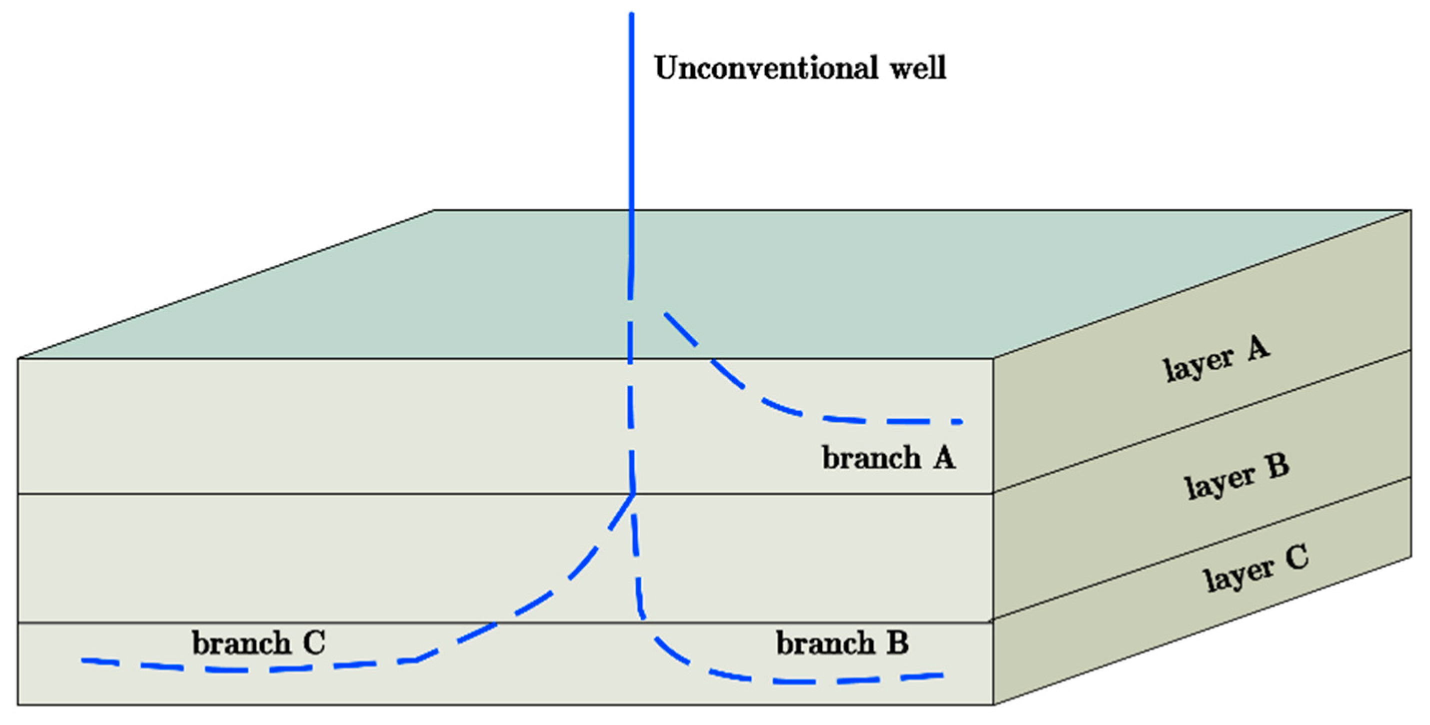
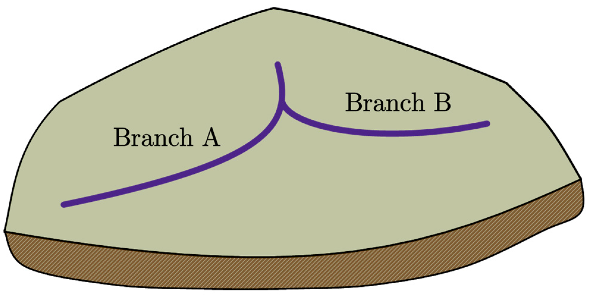
The main indicator for the matching between unconventional well types and reservoirs in this paper depends on the production rate in different producing sections. The producing sections are the part of wellbore where fluid can flow in or out, such as a branch or a step in unconventional wells, as shown in Figure 1.

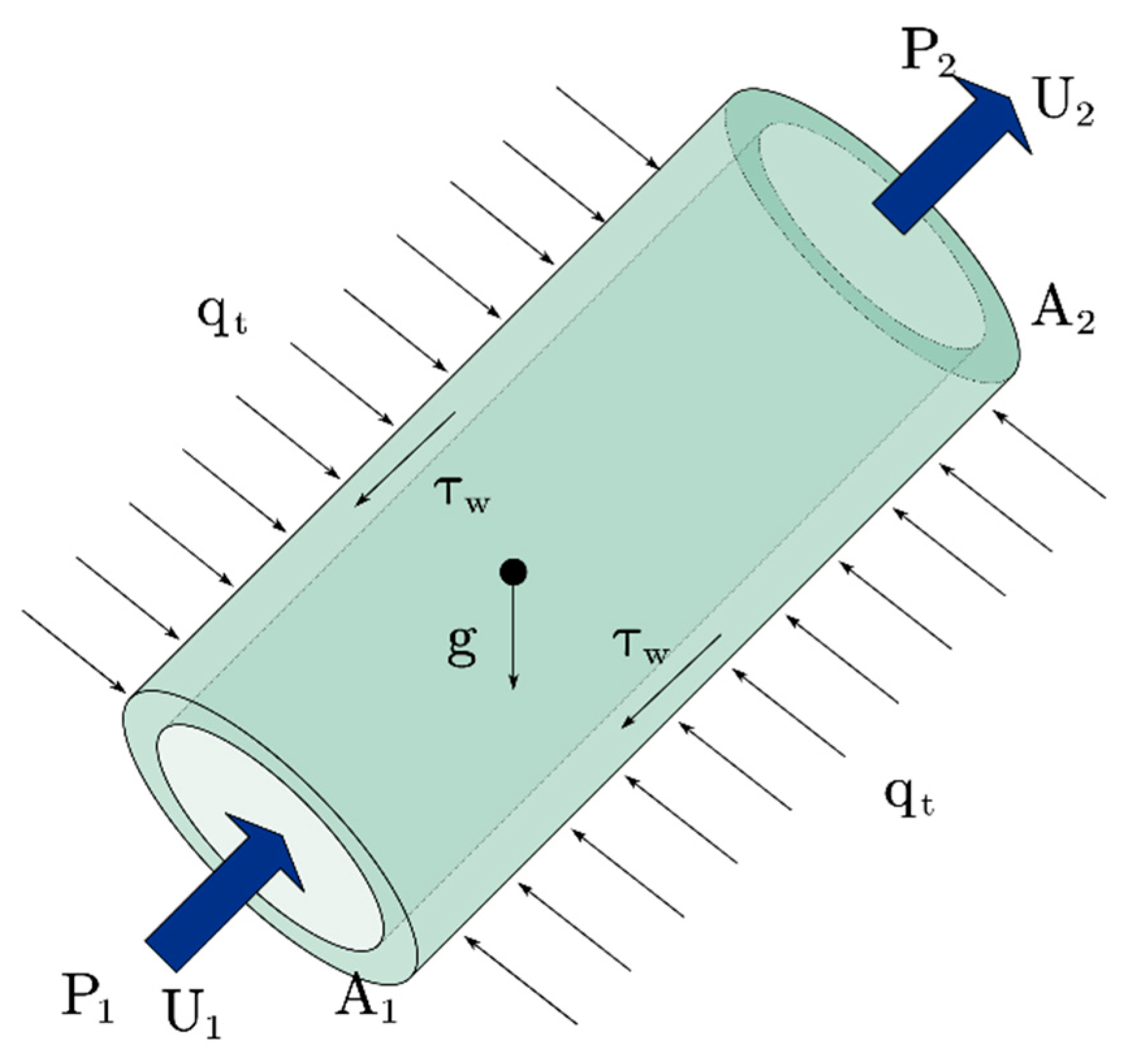
There are many factors affecting the production rate of producing sections, including wellbore flow pressure drop, permeability difference, and viscosity difference between each layer when developing a multilayer reservoir. Therefore, we should choose a suitable model to calculate the production rate of each producing section, which can consider these factors. Han [27] presented a semi-analytical model, which describes the well shape by discretizing the producing section into segments (as shown in Figure 2), treats the reservoir as a box that can be layered (as shown in Figure 3), and considers the coupling between the reservoir and the well.

We assume that there are $n_w$ wells in the reservoir, and for a certain well, $i_w$ has $n_l$ branches, with each branch numbered $i_l$. We discretize each branch into $n_s$ segments, and each segment is numbered $i_s$. The $n_w$, $n_l$, and $n_s$ of the different well types mentioned in this paper are shown in

Table 1. The method of discretization for different unconventional wells.

Unconventional Well Type	${\mathit{n}}_{\mathit{w}}$	${\mathit{n}}_{\mathit{l}}$	${\mathit{n}}_{\mathit{s}}$
Horizontal Wells	1	1	10
Stepped Wells	1	1	10
Multilateral Wells	1	2	10
Fish-bone Wells	1	Arbitrary	Arbitrary

.

2.2. Modeling

In the physical model, we simplify the reservoir as a homogeneous and anisotropic box that can be layered. The fluid in the whole reservoir is simplified to be single-phase and micro-compressible, and the seepage of the fluid follows Darcy’s law. A single unconventional well that has an arbitrary shape and has $n_l$ branches (as shown in Figure 3) is produced in the reservoir. The discrete rule for each branch obeys Table 1.

(1)

Seepage equation

The partial differential equation describing the fluid adiabatic flow is

$$k_x\frac{{\partial }^2\phi }{\partial x^2}+k_y\frac{{\partial }^2\phi }{\partial y^2}+k_z\frac{{\partial }^2\phi }{\partial z^2}=\varphi \mu c_t\frac{\partial \phi }{\partial t}$$

(1)

where $\phi =\mathrm{p}+\rho \mathrm{gh}$. Using potential instead of pressure is included to account for the effect of gravity.

Converting anisotropic reservoirs to isotropic reservoirs using Besson coordinate transformation [28], Equation (1) is rewritten as

$$\frac{{\partial }^2\phi }{\partial x^2}+\frac{{\partial }^2\phi }{\partial y^2}+\frac{{\partial }^2\phi }{\partial z^2}=\frac{\varphi \mu c_t}{k}\frac{\partial \phi }{\partial t}$$

(2)

Using the instantaneous point source solution method intends to obtain a continuous line source solution for line source named $M_0{M}_l$. Appendix A provides the process of the instantaneous point source solution method.

(2)

Variable mass flow equation in wellbore

Adiabatic momentum equation for single-phase incompressible fluids is

$$\frac{dp}{dx}=-2\rho q\frac{U}{A}-{\tau }_w\frac{S}{A}-\rho g\sin \theta$$

(3)

Figure 4 shows the variable mass flow and Equation (3) shows that the pressure drops $\mathsf{\Delta }P$ in the wellbore is composed of three components:

• $\mathsf{\Delta }{P}_a$: pressure drop caused by acceleration;
• $\mathsf{\Delta }{P}_f$: pressure drop caused by friction;
• $\mathsf{\Delta }{P}_g$: pressure drop caused by gravity.

We can calculate $\mathsf{\Delta }{P}_a$, $\mathsf{\Delta }{P}_f$, and $\mathsf{\Delta }{P}_g$ using the methods from some previous studies [29,30,31].

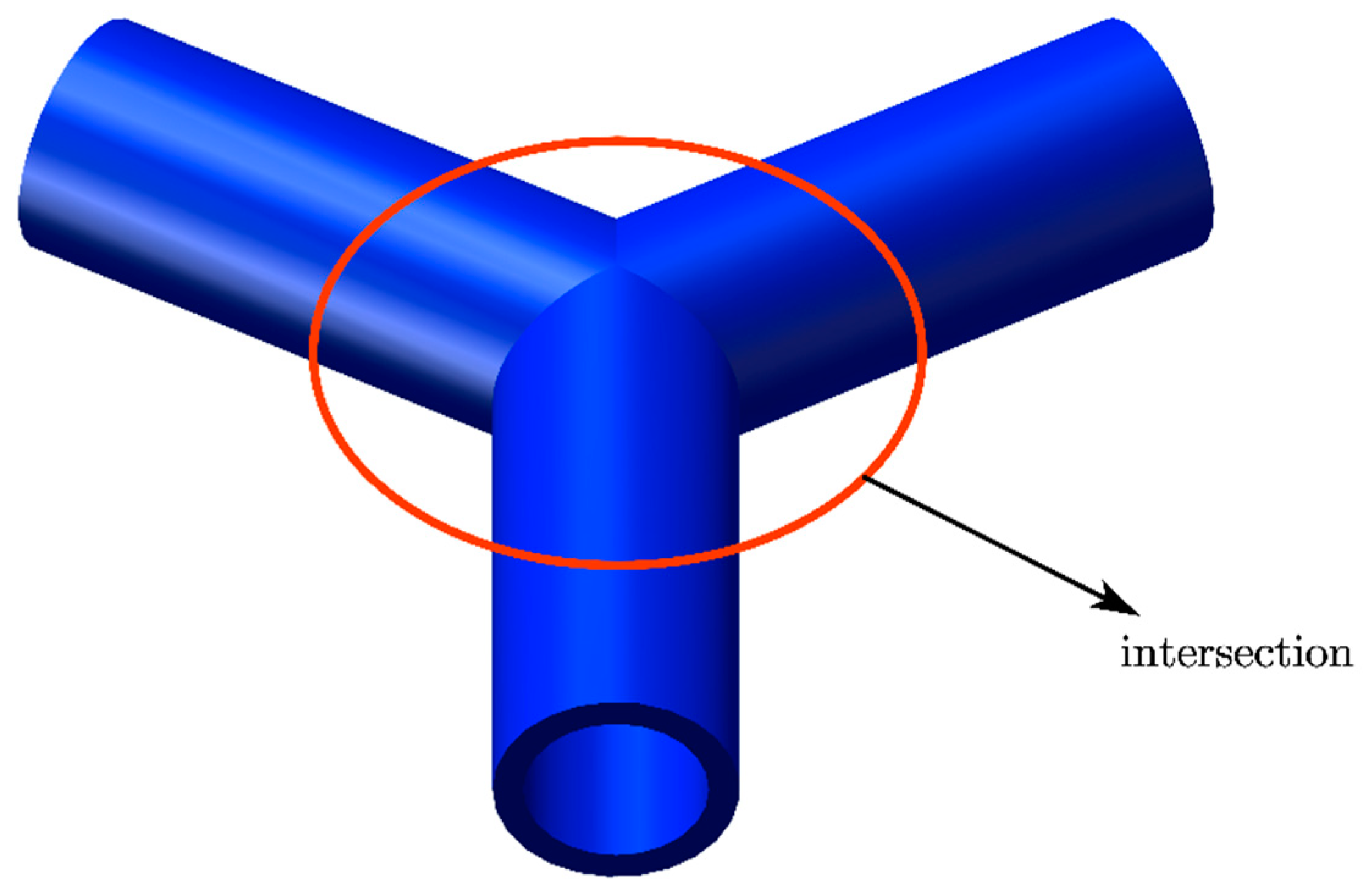
In addition, for multilateral wells, local resistance exists at intersections as shown in Figure 5. The local resistance at an intersection is

$$\Delta P_{\alpha }={10}^{-2}\cdot \frac{3v^2}{2g}\sin \left(\frac{\alpha }{2}\right)$$

(4)

(3)

Coupling model

The coupling model takes each segment as the target, performs a coupled calculation by considering both reservoir seepage and wellbore flow.

We define dimensionless variables as

$$\left\{\begin{array}{c}{\mathrm{t}}_D=\frac{kt}{\varphi \mu c_t{x}_e^2}\\ q_D=\frac{qB\mu }{k{x}_e{\phi }_i}\\ {\phi }_D=\frac{{\phi }_i-\phi }{{\phi }_i}\end{array}\right.$$

(5)

As shown in Figure 2, there are ${2\times n}_w\times n_l\times n_s$ unknown variables in the model, including $n_w\times n_l\times n_s$ inflow and outflow rate $q_{ID}\left(i_w,i_l,i_s\right)$ and $n_w\times n_l\times n_s$ dimensionless potential difference ${\phi }_{wD}\left(i_w,i_l,i_s\right)$. Thus, ${2\times n}_w\times n_l\times n_s$ equations are needed. These equations can be obtained based on mass conservation, potential difference, and flow in the wellbore.

The conservation of mass equation is

$${\displaystyle \sum _{i_l=1}^{n_l(i_w)}{\displaystyle \sum _{i_s=1}^{n_s(i_w,i_l)}{q}_{ID}\left(i_w,i_l,i_s\right)=q_D(i_w)(i_w=1,2,\cdots \cdots .n_w)}}$$

(6)

The potential difference equation is

$$\begin{array}{ll}{\phi }_{wD}\left(i_w,i_l,i_s\right)& =\frac{{\phi }_i-{\phi }_w\left(i_w,i_l,i_s\right)}{{\phi }_i}\\ & ={\displaystyle \sum _{j_w=1}^{n_w}{\displaystyle \sum _{j_l=1}^{n_l(j_w)}{\displaystyle \sum _{j_s=1}^{n_s(j_w,j_l)}{q}_{ID}(j_w,j_l,j_s){\phi }_D(j_w,j_l,j_s)\left[M(i_w,i_l,i_s)\right]}}}\\ & +q_D\left(i_w,i_{\iota },i_s\right)s\left(i_w,i_{\iota },i_s\right)\end{array}$$

(7)

The potential difference equation comes from the solution of the seepage equation by using the instantaneous point source solution method, and we can consider the effect of well completion by introducing a skin factor $s$ in the potential difference equation [32,33]. In addition, Han turned the problem of reservoir heterogeneity into the problem of calculating skin factors near wellbores [34,35,36].

The wellbore flow equation is

$$\begin{array}{ll}{\phi }_{\mathrm{w}}\left(i_w,i_l,i_s+1\right)& ={\phi }_{\mathrm{w}}\left(i_w,i_l,i_s\right)+\Delta p_f\left(i_w,i_l,i_s+1\right)+\Delta p_a\left(i_w,i_l,l_s+1\right)\\ & +\Delta p_g\left(i_w,i_l,i_s+1\right)\end{array}$$

(8)

where

$$\Delta p_f\left(i_w,i_b,i_s,i_s+1\right)=\frac{4{\tau }_w\left(i_w,i_b,i_s,i_s+1\right)}{D}\Delta L\left(i_w,i_b,i_s,i_s+1\right)$$

(9)

$$\Delta p_a\left(i_w,i_l,i_s+1\right)=\frac{2}{A}\rho U{q}_I\Delta L\left(i_w,i_l,i_s+1\right)$$

(10)

$$\Delta p_{\mathrm{g}}\left(i_w,i_l,i_s+1\right)=\rho gA\Delta L\left(i_w,i_l,i_s+1\right)$$

(11)

Then, we can rewrite Equation (8) in a dimensionless form and combine Equations (7) and (8) to find

$$\begin{array}{ll}{\phi }_{\mathrm{wD}}\left(i_w,i_l,i_s+1\right)& ={\phi }_{\mathrm{wD}}\left(i_w,i_{l,}{i}_s\right)+\frac{1}{{\phi }_i}{\displaystyle \sum _{i_b=1}^{i_b-1}{\displaystyle \sum _{i_s=1}^{i_s-1}\left(\Delta p_f+\Delta p_a+\Delta p_g\right)}\left(i_w,i_{b,}{i}_s,i_s+1\right)}\\ & ={\displaystyle \sum _{j_w=1}^{n_w}{\displaystyle \sum _{j_l=1}^{n_l(j_w)}{\displaystyle \sum _{j_s=1}^{n_{s}I{j}_w,j_l)}{q}_{ID}(j_w,j_l,j_s)}}}{\phi }_D(j_w,j_l,j_s)\left[M(i_w,i_l,i_s)\right]\end{array}$$

(12)

For the three types of equations mentioned above, there is one mass conservation equation, $M\times N+1$ potential difference equations, and $M\times N-1$ wellbore flow equations. The number of equations is equal to the number of unknown variables, so the equations are an evenly determined system of equations, and the solution is unique.

2.3. Solving the Model

The model is solved using Ouyang’s method [37]. After obtaining the flow rate in each segment, the potential difference in each segment can be obtained by using Equation (12). Equation (12) can be written in the following form:

$$A\overrightarrow{x}=\overrightarrow{d}$$

(13)

The unknowns vector $\overrightarrow{x}$ is defined as:

$$\overrightarrow{x}={\left[q_{ID}(1,1,1),\cdots \cdots ,q_{ID}(n_w,n_l,n_s),{\phi }_{wD}(1,1,1),\cdots \cdots ,{\phi }_{wD}(n_w,1,1)\right]}^T$$

(14)

The vector $\overrightarrow{d}$ is defined as:

$$\overrightarrow{d}={\left[T(1,1,1),\cdots \cdots ,T(n_w,n_l,n_s),q_D(1),\cdots \cdots ,q_D(n_w)\right]}^T$$

(15)

where

$$T(i_w,i_l,i_s)=-\frac{1}{{\phi }_i}{\displaystyle \sum _{i=1}^{i_s-1}\left(\Delta p_f+\Delta p_a\right)}\left(i_w,i_l,i;i+1\right)$$

(16)

The kernel matrix $A$ is

$$A=\left[\begin{array}{cc}{A}_{11}& A_{12}\\ A_{21}& A_{22}\end{array}\right]$$

(17)

where

$$A_{11}=\left[\begin{array}{cccc}{\varphi }_D(1,1,1)\left[M(1,1,1)\right]& {\varphi }_D(1,1,2)\left[M(1,1,1)\right]& \cdots & {\varphi }_D(n_w,n_l,n_s)\left[M(1,1,1)\right]\\ {\varphi }_D(1,1,1)\left[M(1,1,2)\right]& {\varphi }_D(1,1,2)\left[M(1,1,2)\right]& \cdots & {\varphi }_D(n_w,n_l,n_s)\left[M(1,1,2)\right]\\ \cdots & \cdots & \cdots & \cdots \\ {\varphi }_D(1,1,1)\left[M(1,n_l,n_s)\right]& {\varphi }_D(1,1,2)\left[M(1,n_l,n_s)\right]& \cdots & {\varphi }_D(1,1,1)\left[M(1,n_l,n_s)\right]\\ {\varphi }_D(1,1,1)\left[M(2,1,1)\right]& {\varphi }_D(1,1,2)\left[M(2,1,1)\right]& \cdots & {\varphi }_D(n_w,n_l,n_s)\left[M(2,1,1)\right]\\ \cdots & \cdots & \cdots & \cdots \\ {\varphi }_D(1,1,1)\left[M(2,n_l,n_s)\right]& {\varphi }_D(1,1,2)\left[M(2,n_l,n_s)\right]& \cdots & {\varphi }_D(n_w,n_l,n_s)\left[M(2,n_l,n_s)\right]\\ \cdots & \cdots & \cdots & \cdots \\ \cdots & \cdots & \cdots & \cdots \\ {\varphi }_D(1,1,1)\left[M(n_w,n_l,n_s)\right]& {\varphi }_D(1,1,2)\left[M(n_w,n_l,n_s)\right]& \cdots & {\varphi }_D(n_w,n_l,n_s)\left[M(n_w,n_l,n_s)\right]\end{array}\right]$$

(18)

$$A_{12}=\left[\begin{array}{llllll}-1\hfill & 0\hfill & 0\hfill & \cdots \hfill & 0\hfill & 0\hfill \\ -1\hfill & 0\hfill & 0\hfill & \cdots \hfill & 0\hfill & 0\hfill \\ \cdots \hfill & \cdots \hfill & \cdots \hfill & \cdots \hfill & \cdots \hfill & \cdots \hfill \\ -1\hfill & 0\hfill & 0\hfill & \cdots \hfill & 0\hfill & 0\hfill \\ 0\hfill & -1\hfill & 0\hfill & \cdots \hfill & 0\hfill & 0\hfill \\ \cdots \hfill & \cdots \hfill & \cdots \hfill & \cdots \hfill & \cdots \hfill & \cdots \hfill \\ 0\hfill & -1\hfill & 0\hfill & \cdots \hfill & 0\hfill & 0\hfill \\ \cdots \hfill & \cdots \hfill & \cdots \hfill & \cdots \hfill & \cdots \hfill & \cdots \hfill \\ \cdots \hfill & \cdots \hfill & \cdots \hfill & \cdots \hfill & \cdots \hfill & \cdots \hfill \\ 0\hfill & 0\hfill & 0\hfill & \cdots \hfill & 0\hfill & -1\hfill \end{array}\right]$$

(19)

$$A_{21}=\left[\begin{array}{llllllllllll}1\hfill & \cdots \hfill & 1\hfill & 0\hfill & \cdots \hfill & 0\hfill & 0\hfill & \cdots \hfill & 0\hfill & 0\hfill & \cdots \hfill & 0\hfill \\ 0\hfill & \cdots \hfill & 0\hfill & 1\hfill & \cdots \hfill & 1\hfill & 0\hfill & \cdots \hfill & 0\hfill & 0\hfill & \cdots \hfill & 0\hfill \\ \cdots \hfill & \cdots \hfill & \cdots \hfill & \cdots \hfill & \cdots \hfill & \cdots \hfill & \cdots \hfill & \cdots \hfill & \cdots \hfill & \cdots \hfill & \cdots \hfill & \cdots \hfill \\ \cdots \hfill & \cdots \hfill & \cdots \hfill & \cdots \hfill & \cdots \hfill & \cdots \hfill & \cdots \hfill & \cdots \hfill & \cdots \hfill & \cdots \hfill & \cdots \hfill & \cdots \hfill \\ 0\hfill & \cdots \hfill & 0\hfill & 0\hfill & \cdots \hfill & 0\hfill & 0\hfill & \cdots \hfill & 0\hfill & 1\hfill & \cdots \hfill & 1\hfill \end{array}\right]$$

(20)

The procedure of solving is as follows:

• Solve the conservation of mass equation and potential difference equation ignoring flow in wellbore to obtain the flow rate in each segment.
• Use the result in step 1 and repeat step 1 to calculate the potential difference in each segment.
• Compare the results of each iteration (flow rate and potential difference), stop the iteration if accuracy is sufficient, but otherwise continue iteration.

2.4. Validation of the Model

Validation of the semi-analytical model was performed based on the electrical simulation experimental data and reservoir simulation data from Han’s study [27].

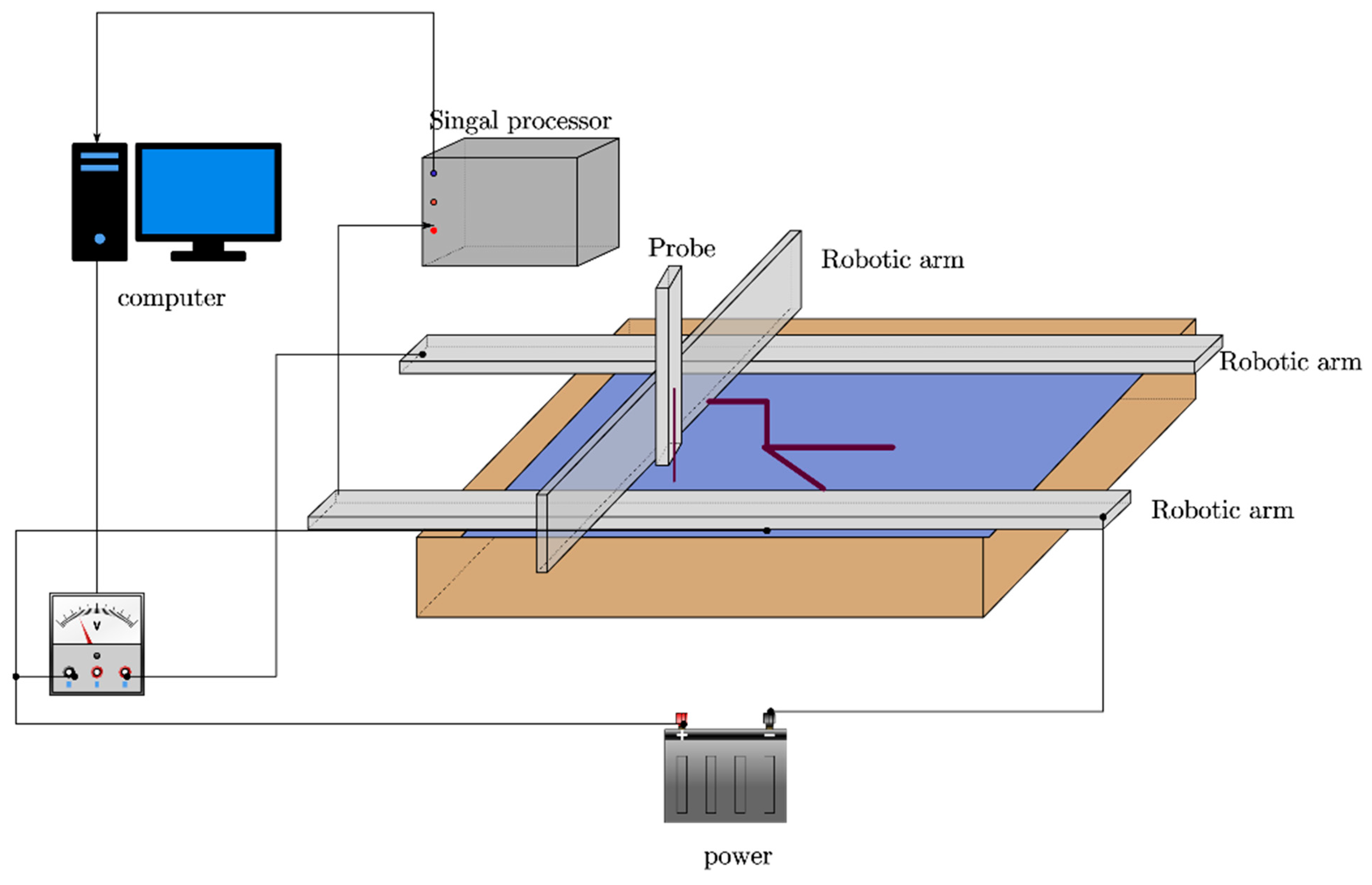
The electrical simulation experiment is a simple and effective method to simulate the seepage in reservoir, which uses brine as a conductive medium, uses the electric field to simulate the seepage field, and uses different shapes and sizes of copper rods to simulate different well types. The theoretical basis of the electrical simulation experiment is the theory of water and electricity similarity [38,39,40]. Figure 6 and Figure 7 show the installation for an electric simulation experiment.

The experimental model and the corresponding actual model parameters are shown in

Table 2. Comparison between the experimental model and the corresponding actual model parameters.

Name	Parameters of Experimental Model (mm)	Parameters of Actual Model (m)
Reservoir Size	740 (Radius)	103.6 (Edge length)
Thickness	109.5	7.66
Well Diameter	2.6/3.0/4.0	0.182/0.21/0.28
Length of Main Wellbore	600	42

.

We define the dimensionless production rate, which means the ratio of the production rate between an actual unconventional well and a vertical well under the same conditions at unit pressure difference, and define the dimensionless current, which means the ratio of current between the experimental model of an unconventional well and vertical well under the same conditions at unit voltage difference. A partial comparison of the experimental results with the semi-analytical model calculations is shown in

Table 3. Comparison of the results between experimental model and semi-analytical model for horizontal wells.

Well Type	Length of Experimental Model Well (m)	Diameter of Experimental Model Well (mm)	Dimensionless Current	Dimensionless Production Rate	Relative Deviation (%)
Horizontal Wells	0.6	4.0	2.73	2.90	6.40
	0.6	2.6	2.61	2.79	7.02

and

Table 4. Comparison of results between experimental model and semi-analytical model for multilateral wells.

Well Type	Branch Length of Experimental Model Well (m)	Diameter of Experimental Model Well (mm)	Angle of Experimental Model Well (°)	Dimensionless Current	Dimensionless Production Rate	Relative Deviation (%)
Multilateral Wells	0.6	4.0	45	3.93	3.99	1.38
	0.4	2.6	90	3.05	3.21	5.13
	0.4	2.6	45	2.76	2.91	5.51
	0.4	2.6	30	2.66	2.78	4.60
	0.4	2.6	10	2.46	2.54	3.21

.

Reservoir simulation can also validate the model. Han used Eclipse as the reservoir simulation software and the semi-analytical model to obtain the inflow profile of wellbore, respectively. The basic parameters are shown in

Table 5. Basic parameters.

Basic Parameters	Values
Reservoir Size (m)	1500 × 1950 × 90
Permeability (mD)	136.25 × 135.33 × 11.74
Porosity (fraction)	25
Initial Pressure (MPa)	25
Fluid Density (kg/m3)	961.5
Fluid Viscosity (cp)	20
Volume Factor (m3/m3)	1.05
Wellbore Radius (m)	0.1

.

The comparison of wellbore inflow profile obtained by reservoir simulation and the semi-analytical model is shown in Figure 8.

The results of experiment and reservoir simulation agree well with the predicted results of the semi-analytical model, so the calculation of the semi-analytical model can be considered accurate.

3. The Method for Matching Unconventional Wells to Reservoirs

In this section, we propose a new method for matching unconventional wells to reservoirs. First, we simplify the reservoir to a box that can be layered, and perform an initial adaptation of unconventional wells and reservoirs. Second, we introduce the concept of matching degree curve and matching interval to provide a quantitative criterion for matching the well type to the reservoir. Next, we introduce some parameters for sensitivity analysis to match the well type and reservoir based on matching degree curve and matching interval. Finally, we make a conclusion and provide a workflow to help readers understand the procedure of this method.

3.1. Reservoir Simplification and Initial Adaptation

In different reservoirs, different well types have different levels of adaption. For example, stepped wells are more suitable for thin interbed reservoirs or massive thick heterogeneous reservoirs because they have two or more horizontal producing sections in different planes as shown in Figure 9. Multilateral wells are more suitable for exploiting single-layer reservoirs spread over a large area because they have two or more branches in the same plane, which can increase the drainage area, as shown in Figure 10.

First, we should simplify the reservoir as a box that can be layered. This reservoir box is rectangular in shape and meets the basic requirements of the model in the previous sections. Then, we propose an initial adaptation for different well types and reservoirs based on

Table 6. Initial adaptation table.

Unconventional Well Type	Reservoir
Horizontal wells	Single thin-layer reservoir
Stepped wells	thin interbed reservoir
	Massive thick-layer reservoir with strongly heterogeneous
Porosity (fraction)	Single thin-layer reservoir with large area
Multilateral wells (Branches in the same plane)	Thin interbed reservoir
	Massive thick-layer reservoir with strongly heterogeneous
Multilateral wells (Branches in the different plane)	Single thin-layer reservoir with large area
	Thin interbed reservoir
	Massive thick-layer reservoir with strongly heterogeneous

.

3.2. Judgement of Matching

There are often two or more producing sections in unconventional wells. Due to a series of factors such as fluid and formation properties in different layers, the production rate in some producing sections may be low, which means that drilling these producing sections is a waste of cost. Therefore, guaranteeing that the inflow differences of each producing section are within an acceptable range is an important indicator to evaluate the degree of matching between well type and reservoir. Based on this, we propose some definitions to measure the difference of production rate in different producing section as follows.

$$q_{ns}=\frac{q_1}{q_2}$$

(21)

$$C{r}_1=\frac{q_1}{q_{all}}$$

(22)

$$C{r}_2=\frac{q_2}{q_{all}}$$

(23)

Among them, $q_1$, $q_2$, and $q_{all}$ denote the production rate in different producing sections and the total production rate, respectively. $q_{ns}$ is the dimensionless production rate, which indicates the ratio of the production rate in adjacent producing sections and reflects the coordinated production degree of each producing section. ${Cr}_1$ and ${Cr}_2$ are the contribution rates of different producing sections.

With modifying parameters of reservoir or fluid, the value of $q_{ns}$, ${Cr}_1$, and ${Cr}_2$ will change, and then we can obtain a curve named the matching degree curve. We set an upper boundary and lower boundary when ${Cr}_1$ or ${Cr}_2$ are equal to 1/3, and at the same time $q_{ns}$ equals 200% or 50%, as shown in Figure 11. The lower and upper boundaries divide the curve into three intervals, as follows:

(1)

When $q_{ns}$ is less than the value of upper boundary and greater than the value of lower boundary, the unconventional well is considered to be well matched to the reservoir, and this interval is named the effective interval.

(2)

When $q_{ns}$ is greater than the upper boundary, the unconventional well is considered to be poorly matched to the reservoir, and this interval is named the upper inefficient interval.

(3)

When $q_{ns}$ is less than the lower boundary, the unconventional well is also considered to be poorly matched with the reservoir, and this interval is named the lower inefficient interval.

It should be noted that only two adjacent producing sections are considered here. For the case of multiple producing sections, the dimensionless production rate of adjacent producing sections can be calculated two by two, and the smallest group is considered as the dimensionless production rate in this case.

3.2.1. Sensitivity Analysis of Matching

We define some parameters called impact parameters, which represent the property of the reservoir, fluid or wellbore that can affect the production rate in each producing section, and we can conduct a sensitivity analysis of matching by setting different impact parameters and using semi-analytical model to calculate. There are two categories of impact parameters: the impact parameters related to reservoir and fluid properties and the impact parameters related to wellbore characteristics.

The impact parameters related to reservoir and fluid properties include permeability difference and viscosity difference, which mainly involve two reservoir characteristics: thin interbed reservoir and massive thick reservoir with strongly heterogeneous features, as shown in Figure 12.

As seen in Figure 12, if the reservoir is a thin interbed reservoir, $k_u$ is the permeability in the upper layer, $k_d$ is the permeability in the lower layer, ${\mu }_u$ is the viscosity in the upper layer, and ${\mu }_d$ is the viscosity in the lower layer. If the reservoir is a massive thick reservoir, $k_u$ is the permeability in the upper region, $k_d$ is the permeability in the lower region, ${\mu }_u$ is the viscosity in the upper region, and ${\mu }_d$ is the viscosity in the lower region.

(1)

Permeability difference

A permeability difference in different layers for thin interbed reservoirs or heterogeneity for massive thick reservoir may lead to different production rates in different producing sections. When we set different permeability differences, $q_{ns}$, ${Cr}_1$, and ${Cr}_2$ will be changed. Therefore, we can obtain a matching degree curve and make a judgement between reservoir and wellbore by the upper boundary and the lower boundary in Figure 11.

We can define permeability differences as follows:

$$k_D=\frac{k_u}{k_d}$$

(24)

where $k_D$ is the permeability difference, $k_u$ is the permeability of the upper layer (or the upper region of one layer), and $k_d$ is the permeability of the lower layer (or the lower region of one layer).

(2)

Viscosity ratio

Like permeability, viscosity is an equally important factor affecting the production rate of producing sections. Similarly, the viscosity ratio is defined as

$${\mu }_{ns}=\pm \frac{{\mu }_{\max }}{{\mu }_{\min }}$$

(25)

where ${\mu }_{ns}$ is the viscosity ratio and ${\mu }_{max}$ and ${\mu }_{min}$ are the fluid viscosities in different layers, and ${\mu }_{max}$ is greater than ${\mu }_{min}$.

Due to the effect of pressure drop along the wellbore, the value of the viscosity ratio when the fluid viscosity in the upper layer is greater than the lower layer and when the fluid viscosity in the lower layer is greater than the upper layer are not equivalent. Therefore, when the fluid viscosity in the lower layer is greater than in the upper layer, the viscosity ratio is defined as a negative value. Conversely, when the fluid viscosity in the lower layer is smaller than in the upper layer, we define the viscosity ratio as a positive value.

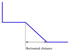
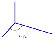
The impact parameters related to wellbore characteristics mainly include height distance, horizontal distance, and branching angle, as shown in Figure 13.

(1)

Height distance

For unconventional wells whose producing sections are not in the same plane, such as stepped wells, the greater the vertical distance between the two producing sections, the greater the pressure drop in the wellbore caused by friction and gravity, which will result in a producing pressure difference in different producing sections, and the producing section in deeper planes may be inefficient or even non-productive. Therefore, the vertical distance between the two producing sections needs to be considered when we decide to use an unconventional well whose producing sections are not in the same plane. In this paper, the vertical distance between the two producing sections is named as height distance, which is one of the impact parameters for well type and reservoir matching.

(2)

Horizontal distance

Similar to the height distance, the greater horizontal distance between the two producing sections, the greater the pressure drop in the wellbore. However, since the increase in horizontal distance only increases the pressure drop caused by friction and has no effect on the pressure drop caused by gravity, the effect of horizontal distance on the matching of well type and reservoirs is not obvious and even negligible when the well production is low.

(3)

Branching angle

When an unconventional well has branches and whose branches are producing in the same layer, interference of the seepage field will exist. The interference will lead to the production rate when these branches develop together being smaller than the sum of the production rate when these branches develop separately. In addition to the matching curve, the analysis of matching for the branching angle also takes the ratio of the production rate when the branches develop together and separately into account. This impact parameter is mainly applicable to multilateral wells and fishbone wells whose branches exploit the same layer.

The list of all impact parameters is shown in

Table 7. The list of all impact parameters.

Impact Parameter Type		Equation or Diagram
Impact parameter related to reservoir	Permeability difference	$K_{\mathrm{ns}}=\frac{K_u}{K_d}$
	Viscosity ratio	${\mu }_{ns}=\pm \frac{{\mu }_{\max }}{{\mu }_{\min }}$
Impact parameter related to wellbore characteristics	Height distance
	Horizontal distance
	Angle

.

3.2.2. Workflow

(1)

Take the reservoir as the object of study and simplify the reservoir as a rectangular box with a single layer or multiple layers. Make an initial adaptation combing reservoir characteristics and referring to Table 6.

(2)

Establish the semi-analytical model for unconventional wells combining reservoir physical properties, fluid properties, and production parameters.

(3)

Controlling the other impact parameters, change a certain impact parameter and substitute it into the semi-analytical model to calculate the production rate of each producing section, further obtaining the matching degree curve.

(4)

Use the matching degree curve based on judgement of the matching we presented above to find the applicable range of the impact parameters. When the matching degree curves are within the “effective interval”, the unconventional wells and reservoirs are considered to be well matched. On the contrary, when the matching degree curve is within the upper inefficient interval or lower inefficient interval, the unconventional well and the reservoir are considered to be poorly matched.

The workflow mentioned above is summarized in Figure 14.

4. Case Analysis

4.1. Reservoir Simplification and Initial Adaptation

We simplify a real thin interbed reservoir as a box-shaped reservoir, which is divided into three layers: an upper layer, middle layer and lower layer. Among them, the middle layer is an impermeable barrier. According to the principle of initial adaptation, stepped wells or multilateral wells whose producing sections are not in the same plane can be selected for exploitation. In this case, we choose the stepped well to exploit the reservoir, and put the producing sections in the upper layer and lower layer, separately. The two producing sections are connected by a blind pipe.

The basic data of the simplified reservoir and well are shown in

Table 8. The basic data of reservoir.

	Upper Layer	Middle Layer	Lower Layer
$\mathrm{Layer}\mathrm{size}(\mathrm{m}$)	2000 × 2000 × 10	2000 × 2000 × 10	2000 × 2000 × 10
$\mathrm{Top}\mathrm{depth}(\mathrm{m}$)	1000	1010	1020
$\mathrm{Permeability}\mathrm{in}\mathrm{x-direction}(\mathrm{m}\mathrm{D}$)	1500	10	1500
$\mathrm{Permeability}\mathrm{in}\mathrm{y-direction}(\mathrm{m}\mathrm{D}$)	1500	10	1500
$\mathrm{Permeability}\mathrm{in}\mathrm{z-direction}(\mathrm{m}\mathrm{D}$)	150	10	150
Porosity	0.3	/	0.3
$\mathrm{Initial}\mathrm{formation}\mathrm{pressure}\left(\mathrm{M}\mathrm{P}\mathrm{a}\right)$	10.1	/	10.3
Rock compressibility $({\mathrm{M}\mathrm{P}\mathrm{a}}^{-1}$)	0.32 × 10−4	/	0.32 × 10−4
Fluid compressibility $({\mathrm{M}\mathrm{P}\mathrm{a}}^{-1}$)	0.002	/	0.002
$\mathrm{Fluid}\mathrm{density}(\mathrm{g}/{\mathrm{c}\mathrm{m}}^3$)	0.925	/	0.925
$\mathrm{Fluid}\mathrm{viscosity}(\mathrm{m}\mathrm{P}\mathrm{a}·\mathrm{s}$)	30	/	30

,

Table 9. The basic data of stepped well.

	Producing Section in Upper Layer	Producing Section in Lower Layer
$\mathrm{Length}(\mathrm{m}$)	200	200
$\mathrm{Tubing}\mathrm{radius}(\mathrm{m}$)	0.06	0.06

and

Table 10. The basic data of production.

	Value
$\mathrm{Bottom}\mathrm{hole}\mathrm{pressure}(\mathrm{M}\mathrm{P}\mathrm{a}$)	9
$\mathrm{Production}\mathrm{time}(\mathrm{d}$)	200

.

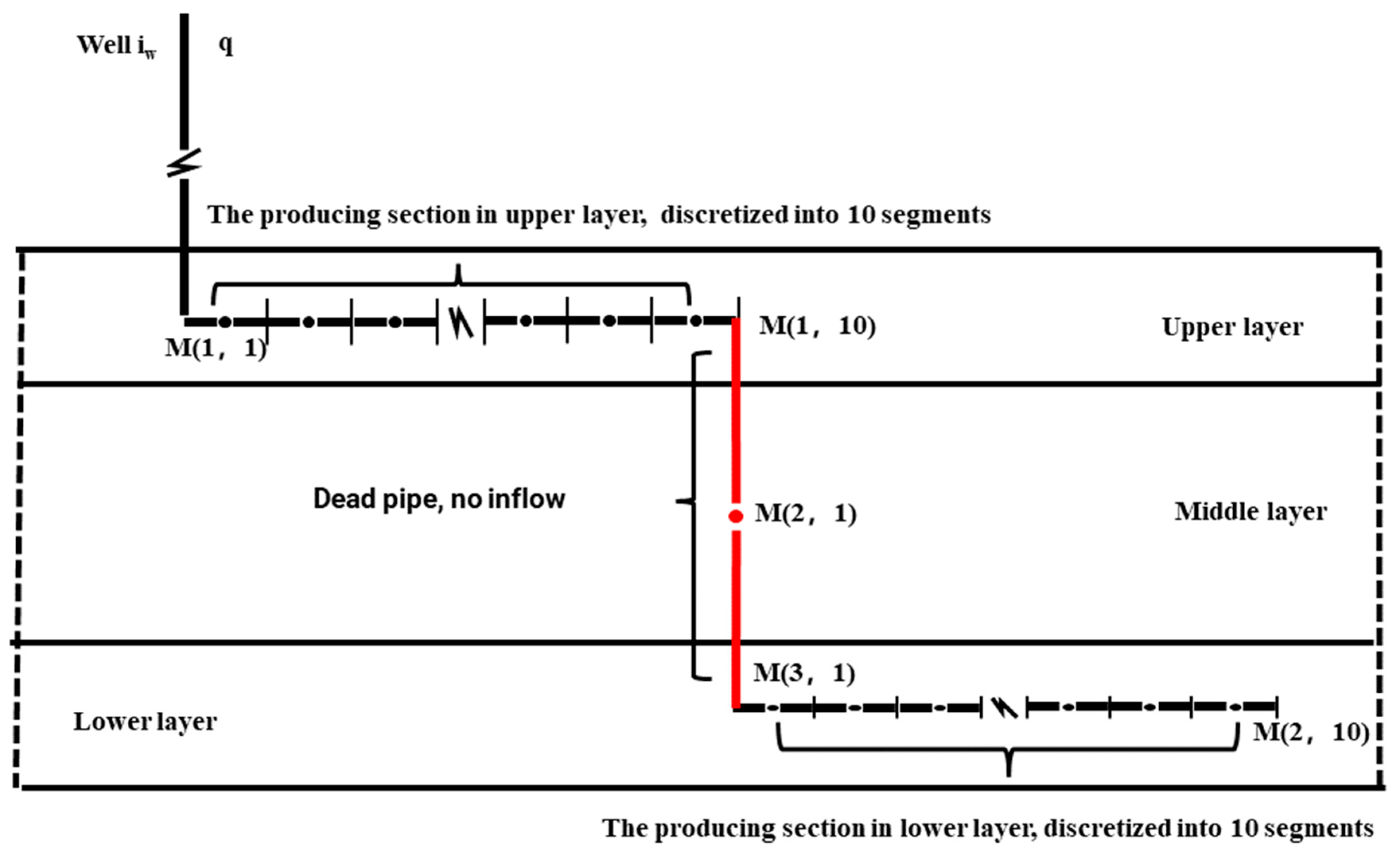
Based on the reservoir and the wellbore description, a semi-analytical model can be developed. The model discretizes each of the two producing sections into ten segments, and the blind tubing section is not discretized. This is shown in Figure 15.

Based on the characteristics of this stepped well and the reservoir, the matching analysis includes four impact parameters: permeability difference, viscosity ratio, height distance, and horizontal distance. The angle between the producing sections is not considered because they are in the same longitudinal plane and do not exploit the same layer.

4.2. Permeability Difference Analysis

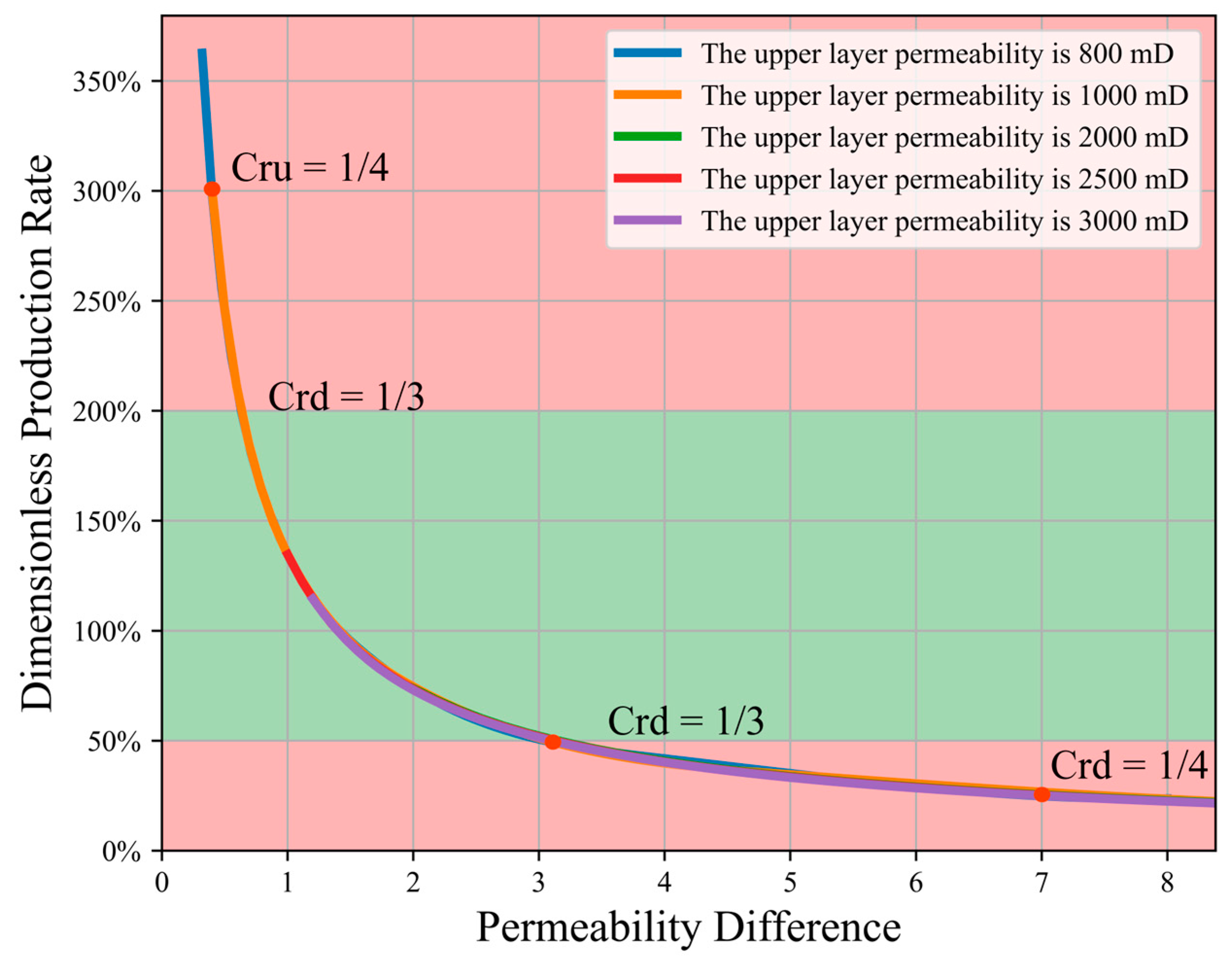
Fixing the permeability in the upper layer and changing the permeability in the lower layer, we can obtain a series of dimensionless production rates. Taking the permeability difference as the X axis and dimensionless production rate as the Y axis, we can obtain a series of points. In this paper, the matching degree curve for the permeability difference is plotted by connecting these points through cubic spline interpolation. Given the dimensionless production rates of 50% and 200%, with substitution into the matching degree curve, we can obtain the matching degree limit of permeability difference. In the image analysis, we use red background and green background to indicate beyond and within matching limits, respectively. Replacing the value of the permeability in the upper layer and repeating the above operation, multiple sets of matching degree curves for the permeability difference can be obtained, as shown in Figure 16.

As shown in Figure 16, the dimensionless production rate shows a decreasing trend as the permeability difference increases, i.e., the greater permeability difference between the lower layer and the upper layer, the worse the matching degree is between the stepped well and the reservoir, and this decreasing trend tends to slow down gradually as the permeability difference increases. The reason is that when the upper layer permeability is fixed, the lower the permeability in the lower layer and the worse the flow ability of fluid is from the lower layer to the wellbore, resulting in a low production contribution from the lower producing section. In addition, the dimensionless production rate is the ratio of two production rates, and when the denominator tends to infinity, the value of the dimensionless production rate will converge to 0. Therefore, as the permeability difference becomes larger, the trend of decreasing the dimensionless production rate becomes slower. Similarly, when the permeability of the lower layer is fixed. The matching degree curves for different permeability values in the upper layer are plotted in the same coordinate system as in Figure 17.

Observing Figure 17, it can be found that the different value of permeability in the upper layer has almost no effect on the shape of the matching degree curve for a certain permeability difference. Therefore, it can be considered that under the current reservoir conditions, regardless of the specific values taken for the permeability in the upper and lower layers, if the value of the permeability difference between the adjacent upper and lower layers is between 0.6 and 3.0, the stepped well can be used for exploitation, i.e., the stepped well is well matched with this thin interbed reservoir in terms of permeability difference. If the permeability difference is not within the effective interval, we think the stepped well is poorly matched with this thin interbed reservoir, and the stepped well is not recommended for exploitation. Since the permeability of the upper and lower layers in this case are equal, i.e., the value of the permeability difference is 1, it can be considered that the stepped well is suitable for the reservoir in the case from the perspective of the permeability difference.

4.3. Viscosity Ratio Analysis

Since the relative values of fluid viscosity in the upper and lower layer directly affect whether the viscosity ratio defined in this paper is positive or negative, only two cases are selected for the analysis of the viscosity ratio in order to unify the positive and negative signs, i.e., the case where the fluid viscosity in the upper layer is less than that in the lower layer (for convenience, we name such reservoirs as ULL) and the case where the fluid viscosity in the upper layer is greater than that in the lower layer (we name such reservoir as UGL).

In this case, the fluid viscosity is 30 mPa∙s, so the fluid viscosity in the upper layer is fixed at 30 mPa∙s, and the fluid viscosity in the lower layer is set as follows: 30, 40, 50, 60, 70, 80, 90, 100, and 110 mPa∙s. We can obtain a series of dimensionless production rates by using the semi-analytical model. Taking the viscosity ratio as the X axis and dimensionless production rate as the Y axis, we can obtain a series of points. Because the fluid viscosity in the upper layer is smaller than or equal to the fluid viscosity in the lower layer at this time, the reservoir in this case is ULL, and the value of the viscosity ratio is specified to be negative in accordance with the viscosity ratio concept mentioned earlier. By connecting these points through cubic spline interpolation, a matching degree curve for the viscosity ratio can be plotted. Given a dimensionless production rate of 50% and 200%, the boundary of the viscosity ratio can be obtained by substituting into the matching degree curve. This is shown in the left panel of Figure 18. Similarly, we can fix the fluid viscosity in the lower layer as 30 mPa∙s, take the fluid viscosity in upper layer as 30, 40, 50, 60, 70, 80, 90, 100, and 110 mPa∙s and repeat the above operation, and we can acquire a matching degree curve for fluid viscosity in UGL. It should be noted that the value of the viscosity ratio is positive, as shown in the right panel of Figure 18.

As shown in Figure 18, the shape and the boundary of the matching degree curve between the ULL reservoir (left figure) and the UGL reservoir (right figure) are different. The former has a larger viscosity ratio threshold. This is because the frictional pressure drop in the producing section in the upper layer is larger than in the lower layer when developing the UGL reservoir, resulting in the producing section in lower layer not having enough production pressure difference to help the fluid flow into the wellbore. Therefore, stepped wells impose higher requirements for UGL reservoirs.

Observing the boundaries in Figure 18, we can conclude that for the reservoir in this case, the viscosity ratio should not exceed 3.03 for the ULL reservoir, i.e., if the fluid viscosity in the upper layer is 30 mPa∙s, the fluid viscosity in the lower layer should not exceed 91 mPa∙s; otherwise, we consider that the stepped well and the reservoir are not well matched, so it is not recommended to use the stepped well to develop this reservoir. Similarly, the viscosity ratio should not exceed 1.56 for the UGL reservoir, i.e., if the fluid viscosity in the lower layer is 30 mPa∙s, the fluid viscosity in the upper layer should not exceed 47 mPa∙s.

Since the fluid viscosity in the upper layer and lower layer are the same in this case, the stepped well is suitable for developing this thin interbed reservoir from the perspective of the viscosity ratio.

4.4. Analysis of Height Distance and Horizontal Distance

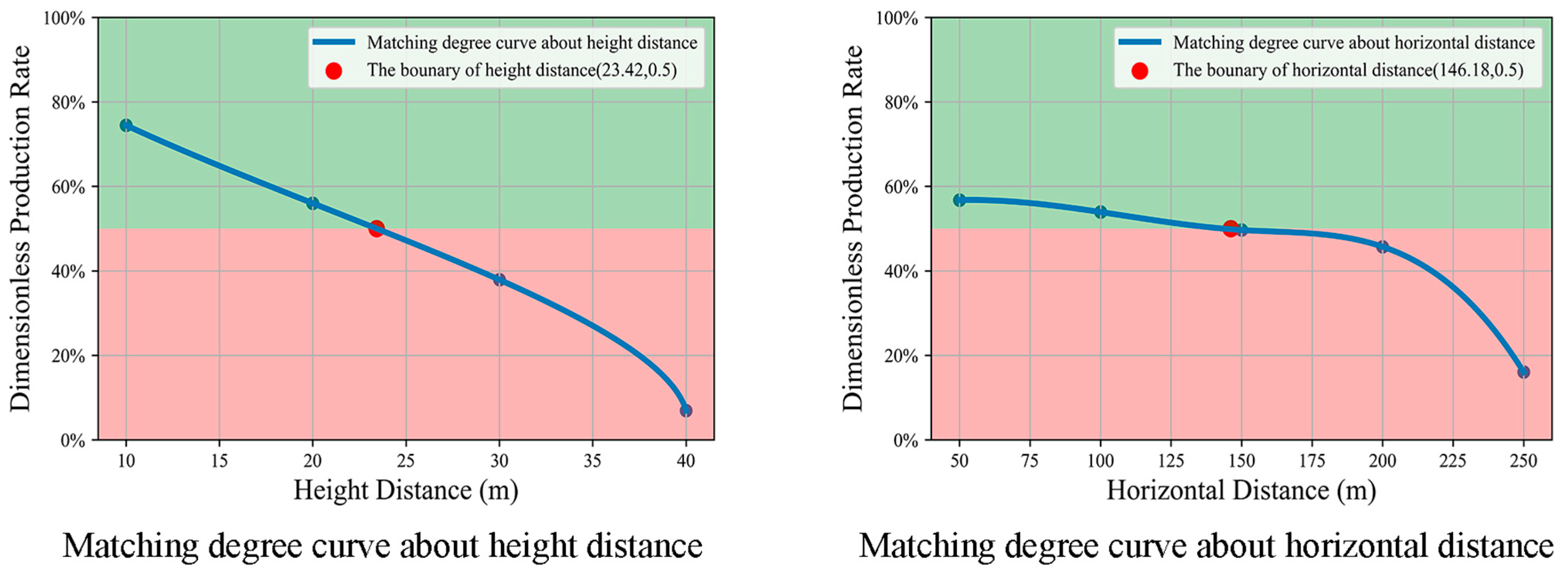
Keeping the other parameters constant, we change the thickness of the compartment and ensure the two producing sections are in the middle depth of the upper and lower layers. The production rate of the producing sections in the upper and lower layers are calculated by the semi-analytical model, and then the matching degree curve and boundaries related to height distance are obtained, as shown in the left panel of Figure 19. Similarly, keeping the other parameters constant and changing the horizontal distance of the two producing sections, we can obtain the matching degree curve and boundaries related to the horizontal distance, as shown in the right panel of Figure 19.

Figure 19 shows that when the height distance does not exceed 23.4 m and the horizontal distance does not exceed 146 m, the stepped well and reservoir are well matched. In this case, the height distance is 20 m and the horizontal distance is 0 m, so we think the stepped well and the reservoir in this case are well matched from the perspective of height distance and horizontal distance. It can also be seen that the height distance between the two producing sections has a much greater effect on the matching of well type and reservoir compared to the horizontal distance. This is because height distance directly affects the gravity pressure drop in the wellbore, which is often much larger than the friction and acceleration pressure drops. Therefore, the height distance of the stepped well needs to be a key consideration.

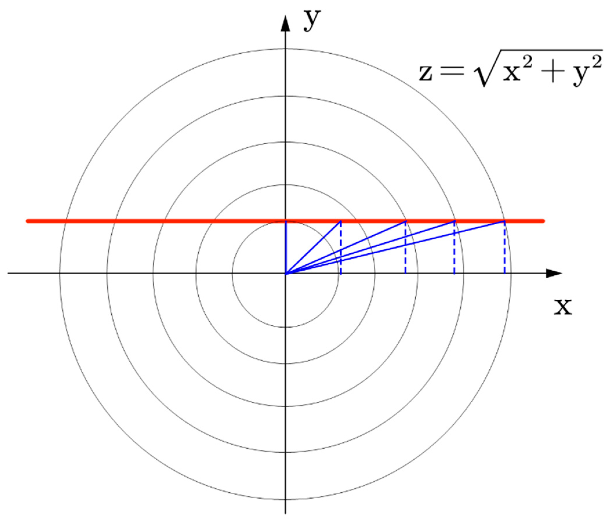
From the right graph of Figure 19, it can be seen that as the horizontal distance increases, the dimensionless production rate decreases gently at first and rapidly later. This is because horizontal distance directly affects the frictional pressure drop, which is proportional to the along-range distance under certain other conditions. We can define $x$ as the horizontal distance, $y$ as the height distance, and $z$ as the along-range distance. The relationship among $x$, $y,$ and $z$ is

$$z=\sqrt{x^2+y^2}$$

(26)

Equation (26) is a circular system equation, and the radius of the circle is z. Keeping $y$ constant, we can obtain a line that is parallel to the $x$ axis, as shown in Figure 20.

Figure 20 shows when $x$ is small, $z$ is mainly influenced by $y$. Since y remains constant, the change in $z$ is not obvious. As $x$ increases, the influence of $y$ on $z$ gradually decreases and the trend of $z$ gradually becomes similar to $x$. It can be imagined easily that when $x$ tends to infinity, the value of $z$ will be almost equal to $x$, and at this time the along-range distance can be approximated as the horizontal distance. The horizontal distance increases, which means that the along-range distance increases identically, and the frictional resistance increases.

4.5. Result

In this case, a thin interbed reservoir is studied for the optimization of unconventional well types, and a stepped well is selected to exploit this reservoir. The degree of matching between the stepped well and reservoir is investigated using the methods proposed in this paper. In summary, the result of this case can be concluded as follows.

• In this method, thin interbed reservoirs need to be simplified as box-shaped reservoirs, which can be layered.
• According to initial adaption, the stepped well is suitable to exploit thin interbed reservoirs;
• Under current reservoir conditions, stepped wells can be used if the permeability difference between the adjacent upper and lower layers is between 0.6 and 3.0. In this case, the permeability difference between the adjacent upper and lower layers is 1, so the stepped well is applicable;
• When the upper fluid viscosity is 30 mPa∙s, the lower fluid viscosity should not exceed 91 mPa∙s, and when the lower fluid viscosity is 30 mPa∙s, the upper fluid viscosity should not exceed 47 mPa∙s. In this case, the fluid viscosity in the upper layer and lower layer are equal to 30 mPa∙s, so the stepped well is applicable;
• When the height distance does not exceed 23.4 m and the horizontal distance does not exceed 146 m, the stepped well and reservoir are well matched. In this case, the height distance is 20 m and the horizontal distance is 0 m, so the stepped well is applicable.

5. Discussion

5.1. Discussion on Model

In this paper, a semi-analytical model is established to calculate the production rate of unconventional wells under different reservoir conditions. The characteristics of this model are summarized as follows:

• Considering the pressure drop in the wellbore and the local resistance in intersections;
• Considering the coupling between the wellbore and reservoir;
• Able to describe the thin interbed and heterogeneous reservoir;
• Able to describe the wellbore with arbitrary shape;
• Considering the effect of well completion.

Using the semi-analytical model for matching unconventional wells and reservoirs is a good idea. On the one hand, we do not need too many parameters to describe the reservoirs and wellbores, and the result is relatively convincing. On the other hand, compared to the numerical model, the semi-analytical model more easily performs sensitivity analysis. However, if we want to describe reservoirs or wellbores more accurately, or describe more complex physical models, we need to conduct more work on modeling. For instance, this model cannot describe reservoirs with arbitrary boundary shapes, multi-media reservoirs, or multi-phase flow in reservoirs or wellbores. We can take a lesson from other research and take more factors into consideration, such as boundary shape [41,42,43], multi-media [44], multi-phase flow [45,46,47,48], temperature distribution in wellbore [49], and other completion methods [50].

5.2. Discussion on the Method for Matching Unconventional Wells to Reservoirs

The method for matching unconventional wells and reservoirs can be divided into two important steps. In the first step, we simplify the reservoir as a box, which can be layered to describe thin interbed reservoirs. Then, we make an initial adaptation between the wellbore and simplified reservoir. In the second step, we build the semi-analytical model based on the first step and define several parameters as quantitative indicators to describe the matching degree between unconventional wells and reservoirs. These quantitative indicators relate to the characteristics of the reservoir and wellbore.

However, if the geological characteristics of a reservoir or the structure of unconventional wells are more complex, the method needs to be expanded further. First, from the perspective of the model, a more comprehensive semi-analytical model needs to be established. Then, we should propose more quantitative indicators as the judgement of matching to analyze the matching degree comprehensively. Finally, some impact parameters involved in this paper need to be modified according to the actual situation.

6. Conclusions

This paper presents a complete analysis method for matching unconventional wells and reservoirs based on semi-analytical models. The method is able to provide a quantitative indicator to describe the matching degree between unconventional wells and reservoirs and is applied to a case. The contributions of this paper are summarized as follows.

• A semi-analytical model is established. This model can describe the shape of well by discretizing the wellbore into segments. A discretization method for some common unconventional wells is provided in this paper, including horizontal wells, stepped wells, multilateral wells, and fishbone wells. In addition, this model takes anisotropic information of reservoirs, variable mass flow in wellbores, and the local resistance at intersections into consideration.
• An initial adaptation reference table for matching unconventional wells and reservoirs is given, which can help engineers to choose a suitable type of unconventional wells for different reservoirs quickly and easily.
• For stepped wells, the height distance has a greater effect on the matching degree than the horizontal distance because of gravity pressure drops. Therefore, we should pay more attention to the height distance when considering using stepped wells.
• When the horizontal distance of the stepped well is short, the pressure drop between the two producing sections is dominated by gravity pressure drop, so the degree of matching is less influenced by horizontal distance. When the horizontal distance is long, the pressure drop between two producing sections is dominated by along-range frictional pressure drop, so the matching degree is more influenced by the horizontal distance.

References

1. Yang, L.; Shi, F.; Zhao, Y. Applied research of complex structure well in shale gas development. Sci. Technol. Eng. 2019, 19, 12–20. [Google Scholar]
2. Shi, P.; Chen, P.; Zhang, Z. Study of completion techniques for unconventional wells. West-China Explor. Eng. 2010, 22, 72–76. [Google Scholar]
3. Sahebi, H.; Wiktorski, E.; Sui, D. Design, Optimization, and Visualization of Wellbore Trajectory in 3D. In Proceedings of the SPE Norway Subsurface Conference, Bergen, Norway, 27 April 2022. [Google Scholar]
4. Al-Dabooni, S.; Tawiq, A.A.; Alshehab, H. Dual Heuristic Dynamic Programming in the Oil and Gas Industry for Trajectory Tracking Control. In Proceedings of the SPE Conference at Oman Petroleum & Energy Show, Muscat, Oman, 21–23 March 2022. [Google Scholar]
5. Alyaev, S.; Daireaux, B. Multi-Trajectory Hydraulic Model for More Accurate Geosteering Constraints. In Proceedings of the SPE/IADC International Drilling Conference and Exhibition, Virtual, 8–12 March 2021. [Google Scholar]
6. Omer, M.; Fragachan, F.E. An Integrated Approach to Optimize Drilling, Completion and Hydraulic Fracturing Performance in Unconventional Wells. In Proceedings of the SPE Annual Technical Conference and Exhibition, Virtual, 26–29 October 2020. [Google Scholar]
7. Reyes, A.; Huang, J.J.; Yuan, Z. Cloud-Based Coherent Wellbore Stability, Improving Trajectory Design for Unconventional Well Construction Planning. In Proceedings of the IADC/SPE International Drilling Conference and Exhibition, Galveston, TX, USA, 3–5 March 2020. [Google Scholar]
8. Dai, Y.; Li, S.; Xia, L. A CBM development well type optimization method based on thelong-run marginal cost. Nat. Gas Ind. B 2018, 38, 113–119. [Google Scholar]
9. Li, X. Geothermal Drilling Well Type Selection and Parameter Optimization Design. Master’s Thesis, Xi’an Shiyou University, Xi’an, China, 2019. [Google Scholar]
10. Boardman, D.W. Designing the Optimal Multi-Lateral Well Type for a Heavy Oil Reservoir in Lake Maracaibo, Venezuela. In Proceedings of the International Thermal Operations and Heavy Oil Symposium, Bakersfield, CA, USA, 10–12 February 1997. [Google Scholar]
11. Lux, M.; Szanyi, J. Effects of vertical anisotropy on optimization of multilateral well geometry. J. Pet. Sci. Eng. 2022, 208, 109424. [Google Scholar] [CrossRef]
12. Almedallah, M.; Altaheini, S.K.; Clark, S. Combined stochastic and discrete simulation to optimise the economics of mixed single-horizontal and multilateral well offshore oil developments. Pet. Explor. Dev. 2021, 48, 1183–1197. [Google Scholar] [CrossRef]
13. Lyu, Z.; Song, X.; Geng, L. Optimization of multilateral well configuration in fractured reservoirs. J. Pet. Sci. Eng. 2019, 172, 1153–1164. [Google Scholar] [CrossRef]
14. Lu, R.; Reynolds, A.C. Joint Optimization of Well Locations, Types, Drilling Order, and Controls Given a Set of Potential Drilling Paths. SPE J. 2020, 25, 1285–1306. [Google Scholar] [CrossRef]
15. Yeten, B.; Durlofsky, L.J.; Aziz, K. Optimization of Nonconventional Well Type, Location, and Trajectory. SPE J. 2003, 8, 200–210. [Google Scholar] [CrossRef]
16. Robertson, E.; Iyer, N.; Klenner, R. Optimization of Unconventional Well-Pad Area Using Reservoir Simulation and Intelligent Sequential Sampling. In Proceedings of the SPE/AAPG/SEG Unconventional Resources Technology Conference, Austin, TX, USA, 24–26 July 2017. [Google Scholar]
17. Rafiee, J.; Sarma, P.; Zhao, Y. Combining Machine Learning and Physics for Robust Optimization of Completion Design and Well Location of Unconventional Wells. In Proceedings of the International Petroleum Technology Conference, Riyadh, Saudi Arabia, 21–23 February 2022. [Google Scholar]
18. Cao, R.; Liu, C.; Brennan, C. Understand the Early Indicators for Long-Term Performance of Unconventional Wells. In Proceedings of the SPE/AAPG/SEG Unconventional Resources Technology Conference, Houston, TX, USA, 23–25 July 2018. [Google Scholar]
19. Carpenter, C. Production Metrics To Predict Long-Term Performance of Unconventional Wells. J. Pet. Technol. 2017, 69, 73–75. [Google Scholar] [CrossRef]
20. Rui, Z.; Cui, K.; Wang, X. A quantitative framework for evaluating unconventional well development. J. Pet. Sci. Eng. 2018, 166, 900–905. [Google Scholar] [CrossRef]
21. Li, R.; Huang, Y.; Li, Y. Research progress of reservoir seepage model and numericalsimulation technology. Petrochem. Ind. Appl. 2021, 40, 11–15+29. [Google Scholar]
22. Zhang, Y.; Ge, H.; Zhao, K. Simulation of pressure response resulted from non-uniform fracture network communication and its application to interwell-fracturing interference in shale oil reservoirs. Geomech. Geophys. Geo-Energy Geo-Resour. 2022, 8, 114. [Google Scholar] [CrossRef]
23. Kelvin, L. Mathematical and Physical Papers; Cambridge University Press: London, UK, 2011. [Google Scholar]
24. Hantush, M.S.; Jacob, C.E. Non-steady radial flow in an infinite leaky aquifer. Eos Trans. Am. Geophys. Union 1955, 36, 95–100. [Google Scholar] [CrossRef]
25. Nisle, R.G. The Effect of Partial Penetration on Pressure Build-Up in Oil Wells. Trans. AIME 1958, 213, 85–90. [Google Scholar] [CrossRef]
26. Horne, R.N.; Temeng, K.O. Relative Productivities and Pressure Transient Modeling of Horizontal Wells with Multiple Fractures. In Proceedings of the Middle East Oil Show, Manama, Bahrain, 11–14 March 1995. [Google Scholar]
27. Han, G. Semi-Analytical Integrated Prediction Model for Unconventional Wells. Doctoral Thesis, China University of Petroleum, Beijing, China, 2004. [Google Scholar]
28. Besson, J. Performance of Slanted and Horizontal Wells on an Anisotropic Medium. In Proceedings of the European Petroleum Conference, The Hague, The Netherlands, 21–24 October 1990; Available online: https://onepetro.org/SPEEURO/proceedings/90EUR/All-90EUR/SPE-20965-MS/67973 (accessed on 5 October 2022).
29. Schulkes, R.; Utvik, O.H. Pressure Drop in a Perforated Pipe With Radial Inflow: Single-Phase Flow. SPE J. 1998, 3, 77–85. [Google Scholar] [CrossRef]
30. Yuan, H.; Sarica, C.; Brill, J.P. Effect of Completion Geometry and Phasing on Single-Phase Liquid Flow Behavior in Horizontal Wells. In Proceedings of the SPE Annual Technical Conference and Exhibition, New Orleans, Louisiana, 27–30 September 1998. [Google Scholar]
31. Yuan, H.J.; Sarica, C.; Brill, J.P. Effect of Perforation Density on Single-Phase Liquid Flow Behavior in Horizontal Wells. SPE Prod. Facil. 1999, 14, 203–209. [Google Scholar] [CrossRef]
32. Unneland, T. An Improved Model for Predicting High-Rate Cased-Hole Gravel-Pack Well Performance. In Proceedings of the SPE European Formation Damage Conference, The Hague, The Netherlands, 31 May–1 June 1999. [Google Scholar]
33. Furui, K.; Zhu, D.; Hill, A.D. A Comprehensive Model of Horizontal Well Completion Performance. In Proceedings of the Spe Technical Conference & Exhibition, Denver, Colorado, 5–8 October 2003; pp. 207–220. [Google Scholar]
34. Peaceman, D.W. Interpretation of well-block pressures in numerical reservoir simulation. SPE J. 1978, 18, 183–194. [Google Scholar]
35. Holmes, J.A.; Barkve, T.; Lund, O. Application of a Multisegment Well Model to Simulate Flow in Advanced Wells. In Proceedings of the European Petroleum Conference, The Hague, The Netherlands, 20–22 October 1998. [Google Scholar]
36. Hawkins, M. A Note on the Skin Effect. Trans. AIME 1956, 207, 65–66. [Google Scholar] [CrossRef]
37. Ouyang, L.B.; Aziz, K. A Simplified Approach to Couple Wellbore Flow and Reservoir Inflow for Arbitrary Well Configurations. Procrrdings of the SPE Annual Technical Conference and Exhibition, New Orleans, Louisiana, 27–30 September 1998. [Google Scholar]
38. Yildiz, T.; Deniz, O. Experimental Study on the Productivity of Complex Well Configurations. In Proceedings of the SPE International Conference on Horizontal Well Technology, Calgary, AB, Canada, 1–4 November 1998. [Google Scholar]
39. Jia, Z.; Li, H.; Song, X. Electrical simulation study of pressure distribution in horizontal wells. J. DaQing Pet. Inst. 1994, 27–30. [Google Scholar]
40. Qu, Z.; Xu, X.; Liu, J. Electric analogy experiment of the productivity of radia-l distributing mult-i branch horizontal wells. J. Xi’an Shiyou Univ. 2007, 65–68+71+3. [Google Scholar]
41. Idorenyin, E.H.; Shirif, E.E. Transient Response in Arbitrary-Shaped Composite Reservoirs. SPE Reserv. Eval. Eng. 2017, 20, 752–764. [Google Scholar] [CrossRef]
42. Jia, P.; Cheng, L.; Huang, S. A comprehensive model combining Laplace-transform finite-difference and boundary-element method for the flow behavior of a two-zone system with discrete fracture network. J. Hydrol. 2017, 551, 453–469. [Google Scholar] [CrossRef]
43. Wang, J.; Wang, X.; Dong, W. Rate decline curves analysis of multiple-fractured horizontal wells in heterogeneous reservoirs. J. Hydrol. 2017, 553, 527–539. [Google Scholar] [CrossRef]
44. Li, Z.; Wu, X.; Han, G. Transient Pressure Analysis of Volume-Fractured Horizontal Wells Considering Complex Fracture Networks and Stress Sensitivity in Tight Reservoirs. ACS Omega 2019, 4, 14466–14477. [Google Scholar] [CrossRef] [Green Version]
45. Zhang, F.; Emami-Meybodi, H. A type-curve method for two-phase flowback analysis in hydraulically fractured hydrocarbon reservoirs. J. Pet. Sci. Eng. 2022, 209, 109912. [Google Scholar] [CrossRef]
46. Zhang, F.; Emami-Meybodi, H. Semianalytical method of two-phase liquid transport in shale reservoirs and its application in fracture characterization. AIChE J. 2022, 68, e17449. [Google Scholar] [CrossRef]
47. Zhang, F.; Emami-Meybodi, H. A Semianalytical Method for Two-Phase Flowback Rate-Transient Analysis in Shale Gas Reservoirs. SPE J. 2020, 25, 1599–1622. [Google Scholar] [CrossRef]
48. Zhang, Z.; Wang, X.; Xiong, Y.; Peng, G.; Wang, G.; Lu, J.; Zhong, L.; Wang, J.; Yan, Z.; Wei, R. Study on borehole temperature distribution when the well-kick and the well-leakage occurs simultaneously during geothermal well drilling. Geothermics 2022, 104, 102441. [Google Scholar] [CrossRef]
49. Tan, M.; Li, Y.; Qi, M.; Wang, H.; Wang, Y.; Lu, J.; Chen, M.; Wu, H. A novel multi-path sand-control screen and its application in gravel packing of deepwater horizontal gas wells. Nat. Gas Ind. B 2022, 9, 376–382. [Google Scholar] [CrossRef]
50. Lu, J.; Jin, G.; Li, D.; Liang, D.; He, Y.; Shi, L.; Zhang, Y.; Xiong, Y. Numerical Simulation on Sand Production Based on Laboratory Gas Hydrate Production Experiment. J. Mar. Sci. Eng. 2023, 11, 110. [Google Scholar] [CrossRef]
Figure 1. Definition of producing section.
Energies 16 03207 g001
Figure 2. Schematic diagram of wellbore segmentation in semi-analytical model.
Energies 16 03207 g002
Figure 3. Schematic diagram of reservoir layering in semi-analytical model.
Energies 16 03207 g003
Figure 4. Diagram of wellbore fluid flow.
Energies 16 03207 g004
Figure 5. Schematic diagram of intersection.
Energies 16 03207 g005
Figure 6. Physical diagram of electric simulation experiment.
Energies 16 03207 g006
Figure 7. Electric simulation experimental schematic diagram.
Energies 16 03207 g007
Figure 8. Inflow profile of wellbore.
Energies 16 03207 g008
Figure 9. Double stepped well in thin interbed reservoir and massive thick reservoir with strongly heterogeneous features.
Energies 16 03207 g009
Figure 10. Multilateral well in single-layer reservoirs with large area.
Energies 16 03207 g010
Figure 11. Matching degree curve and three intervals.
Energies 16 03207 g011
Figure 12. Two simplified reservoir characteristics and corresponding parameters.
Energies 16 03207 g012
Figure 13. Impact parameters related to wellbore characteristics.
Energies 16 03207 g013
Figure 14. Flow chart of matching method between unconventional wells and reservoir.
Energies 16 03207 g014
Figure 15. Schematic diagram of simplified reservoir and stepped well in the case.
Energies 16 03207 g015
Figure 16. Matching degree curve for permeability difference when we change lower layer permeability.
Energies 16 03207 g016
Figure 17. Matching degree curve for permeability difference when change the upper layer permeability.
Energies 16 03207 g017
Figure 18. Matching degree curve about viscosity ratio.
Energies 16 03207 g018
Figure 19. Matching degree curve for height distance and horizontal distance.
Energies 16 03207 g019
Figure 20. Circular system equation.
Energies 16 03207 g020