Characterization of the Hydropower Inlet Effect on the Electric Network Frequency

Abstract

One of the challenges posed by renewable energies is the stabilization of parameters related to the quality of electrical energy. This study demonstrates the existence of a relationship between input blocks of hydropower and the variation of the fundamental frequency of the electricity grid. By mapping production data provided by the Spanish Electric Network with frequency measured in the laboratory, it is shown that gradients of hydropower are correlated with frequency fluctuations for certain characteristic times. Considering hourly instances of energy input, the study compares two methods for calculating hydropower gradients (linear regression and pseudo-linear regression) and two methods for calculating local frequency extrema (the “specular inertia” method and analysis by comparison with the moving average) in order to corroborate the results.

1. Introduction

The electricity grid is a complex system that interconnects generators and consumers of electricity through transmission and distribution infrastructure. The frequency of the supplied voltage is thus a critical parameter that must be kept constant and resilient despite the numerous factors that affect its stability. In the context of an electricity grid, resilience means the ability to withstand and reduce the magnitude and/or duration of disruptive events, including the capability to anticipate, absorb, adapt to, and/or rapidly recover from such an event. Indeed, variations in the frequency of the electrical grid can have serious consequences at the local and large-scale levels, including blackouts and damage to electrical equipment [1,2]. To be more concise, the frequency range for synchronous systems imposed by the UNE-EN 50160:2011 standard for synchronized networks is the following [3]:

• 50 Hz ± 1% during 99.5% of the year.
• 50 Hz + 4%/− 6% during 100% of the time.

This standard also mentions that the frequency must be measured using 10-s periods.

In the last decade, a considerable increase in frequency fluctuations in the grid has been detected, mainly due to the penetration of distributed renewable energy sources [4] and synchronous generators being replaced by power inverters. This is primarily due to the global reduction of grid inertia: converter-based generators have a much lower inertia than a rotating synchronous generator, and thus lead to a greater degree of instability in the electricity grid frequency [5]. Additionally, certain renewable energy sources, such as solar photovoltaic or wind power, are unpredictable, fluctuate, and introduce new terms of randomness in addition to traditional sources of internal noise into the process of stability characterization [6,7].

Nonetheless, not all the energy sources will act the same way on the frequency behaviour. This paper attempts to characterize the difference regarding the energy sources that have been known to have a major correlation with the electricity grid frequency.

Unscheduled energy demand also affects grid stability. For example, during high demand periods, such as peak hours, generation may not be sufficient to meet it, causing subsequent frequency fluctuations. Therefore, adequate control and automatic regulation systems are necessary to maintain a sufficient level of relative stability. In these systems, monitoring, analysis, and characterization of the fluctuation pattern play a crucial role [8,9].

In this paper, after performing a data analysis with MATLAB^TM, the hourly points of maximum and minimum frequency were detected using two different algorithms. The frequency data was obtained based on the methods described in previous work [10]. Analyzing the production data provided by the official website of the Spanish Electric Network, we searched for a relationship between different energy sources, including renewable sources (wind, solar photovoltaic, hydropower, and solar thermal), and combined-cycle power plants [11].

The results show that the gradient of hydropower is correlated with the appearance of the aforementioned local frequency maxima and minima; while the gradient is positive, the tendency is the appearance of maxima, with the same relationship between the negative gradient and minima.

On the one hand, this characterization will allow for quantitative information on the range of frequency variation in a real case. On the other hand, correction mechanisms for corrective maintenance actions can be implemented based on the models.

The paper is structured as follows: After this introduction, the methodology is presented in the next section. Section 3 details the interpretation of the results obtained and is subsequently discussed. Finally, the conclusions are drawn in Section 4.

2. Experimental Methodology

Two datasets have been used: measurements of the frequency and production data of the grid.

The former is extracted from a database of the research group PAIDI-TIC-168 at the University of Cadiz. This dataset collects the values of the grid frequency measured every 10 s online.

The second dataset collects grid power production data, which includes real, forecasted, and scheduled power, as well as power generated from different energy sources (nuclear, coal, combined-cycle, renewables, etc.) [12].

First, the network signal was acquired at the Algeciras Technical School of Engineering (Algeciras, Spain) using hardware, which essentially consists of a chassis and a data acquisition card (DAQ) from the manufacturer NI™, which receives on one hand the voltage input (50 Hz, 230 V RMS) of the electricity grid, and, on the other hand, the pulsed signal (1 PPS) from the GPS receiver (Symmetricon™) [10].

Once the frequency signal was obtained, several sudden fluctuations in the instantaneous frequency of the grid were identified, which occurred during the hourly blocks of the electricity market, i.e., during peak hours.

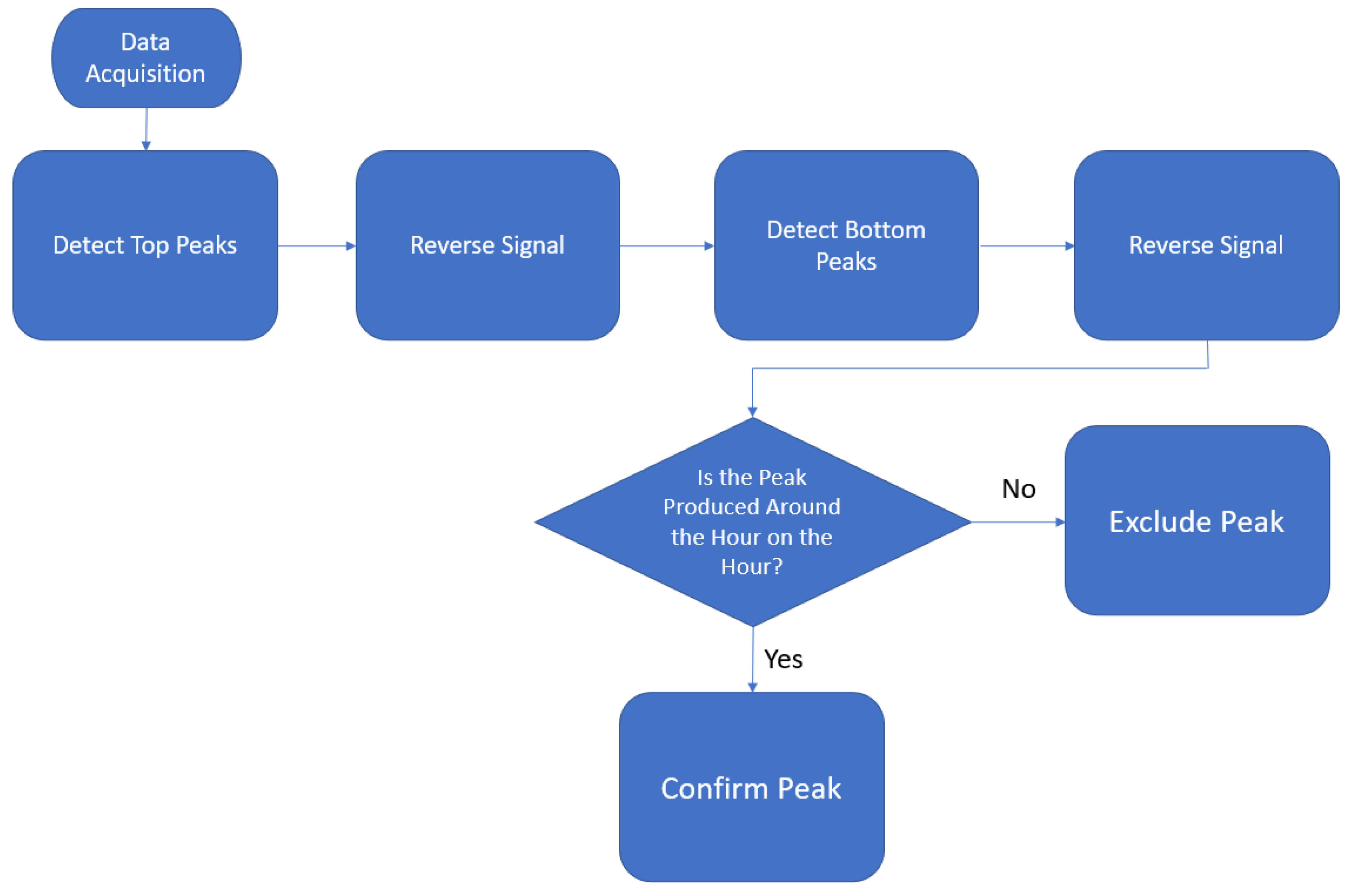
In order to search for fluctuations or “peaks,” it is mandatory that we first define this concept. In this paper, we understand a peak as a local maximum or minimum that surpasses a certain threshold imposed by our algorithms and it is produced in an hour on the hour. That threshold is lower than the actual limits imposed by the norm, so we can thoroughly study not only the points that fall outside the norm but also the potential points that can provoke that situation.

Two algorithms have been programmed to search for these changes using MATLAB^TM software, which are detailed below:

• “Specular inertia” method:
  • This method is based on stabilizing signals with weak damping around a final value. An algorithm was developed using the MATLAB^TM (2022b version, MathWorks) function “Findpeaks”, which locates local extrema. The method identifies the first location using the “MinPeakHeight” and “MinPeakDistance” parameters of the “findpeaks” function, and identifies the second location by first inverting the signal so that the local minimum of the signal becomes the local maximum, and then using the same parameters to locate the R peak. Under these conditions, a search for these extrema was performed, and the algorithm identified the following extrema over the course of a month.
• Comparison with the moving average-based method:
  • This method is based on comparing the 10-min moving average of the frequency with the current value in conjunction with an absolute extremum finder algorithm, working within a certain time window. If the comparison value at the absolute extremum between the moving average and the actual signal exceeds a certain threshold and falls within the range of an hourly block in the electricity market, at each hour on the hour, it is identified as a local maximum or minimum extremum, depending on its value.

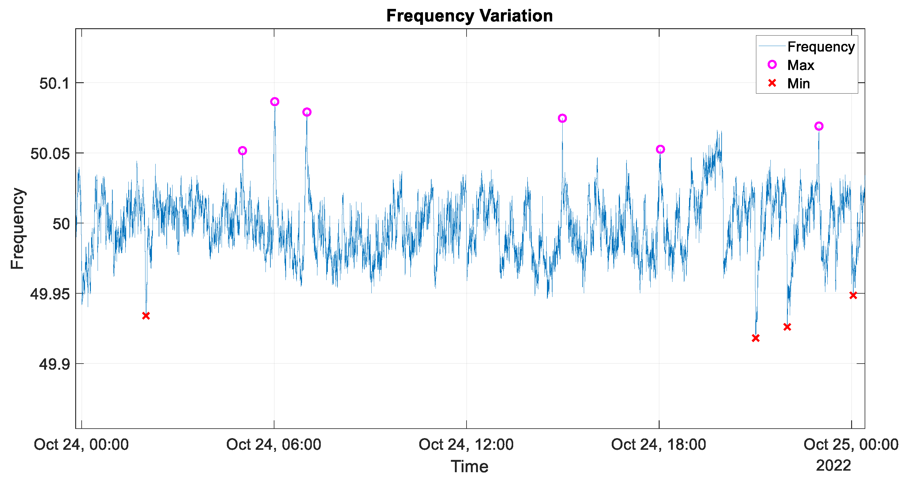
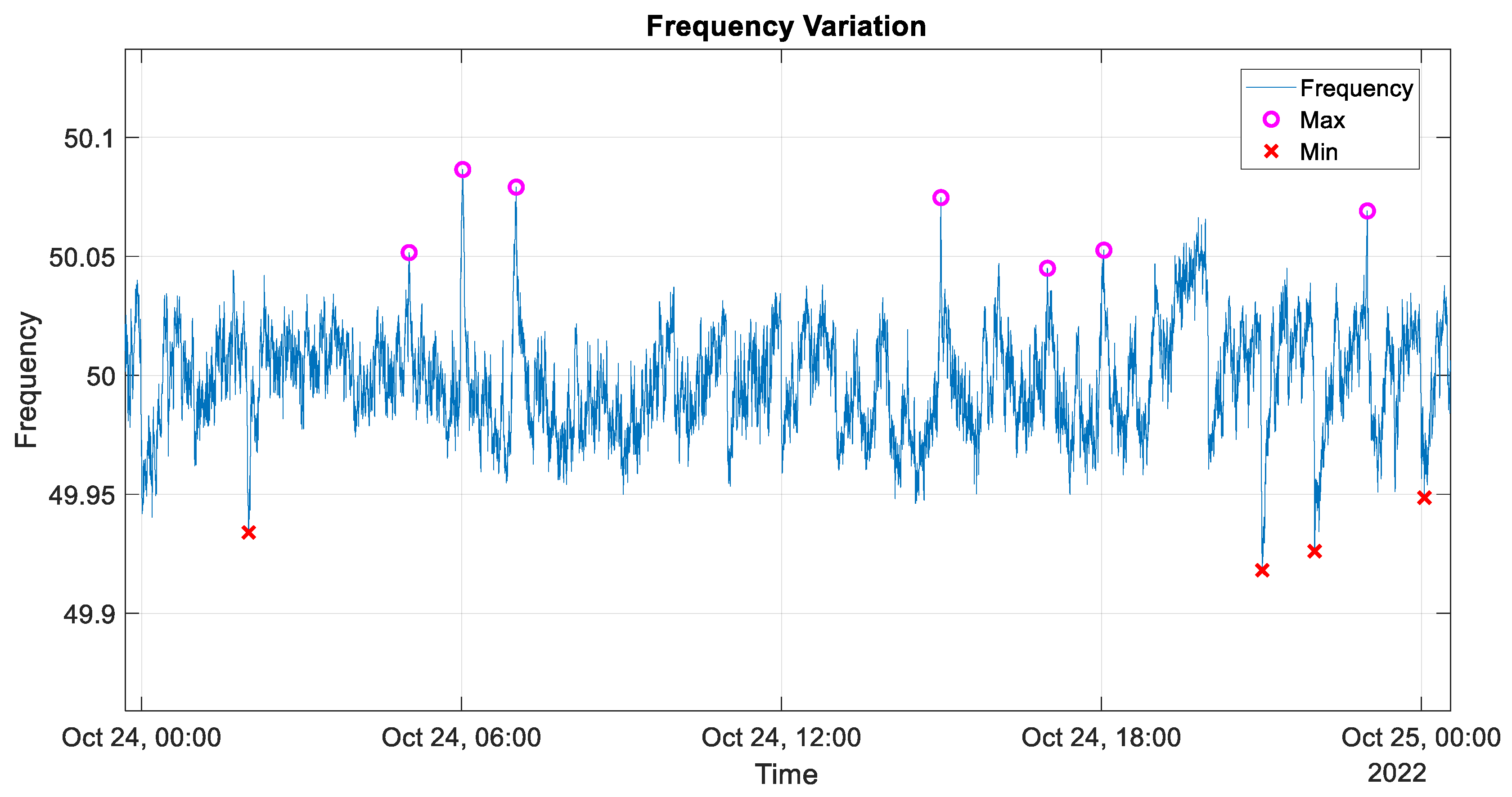
In Figure 1 and Figure 2 we appreciate the flowchart of the “specular inertia method” and the detected points with the algorythm, whereas in Figure 3 and Figure 4 we witness the same information but for the comparison with the moving average-based method.

As a clarification, in Figure 2 and Figure 4, there are several detected points whose peaks are extremely narrow. This is due to both the scale of the image and the sample time of the frequency data (10 s).

It is also important to note that grid frequency is somewhat a measure of the grid’s health, as it reflects its ability to balance and correct differences between supply and demand. In this context, inertia has historically been an important issue of reliability in the electric grid. Indeed, rotating electrical generators in fossil and hydroelectric power plants (and eventually in nuclear power plants) represent sources of stored energy that is usually withdrawn for a few seconds to provide the grid time to respond to the power plant or other system failures. This is why, in this paper, the sharpness of the peaks provides a qualitative indication of the grid inertia. Inertia is negligible for renewable resources in comparison with hydropower [4,5].

Later on, the gradient of hydropower will be used to test the hypothesis that maxima tend to occur in situations where there is an increase in hydropower, and conversely, where there are minima, there is a decrease in hydropower.

To calculate this gradient, production data, which is provided every 5 min, is used. The objective is to obtain an average gradient per hour in order to compare it with the hourly maxima and minima and determine the average slope at which they occur.

Since there are 12 production data points in an hour (one every 5 min), they are divided into 3 blocks of 4 data points. The average of each block is calculated, and with those 3 averages, the increase of the first block average with the second block average and the increase of the second block average with the third block average are calculated, concluding with the average of both increases. This average will be the hourly value of the gradient used in subsequent sections. Figure 5 graphically represents the described method with an example dataset.

With the MATLAB^TM function “Polyfit,” we obtain the coefficients of the regression line of the analyzed data by means of the following line of code.

[r,~,mu] = polyfit(minute,Hydropower,1);

The polyfit function is given as input the time base, the hydroelectric power, and one, which refers to the degree of the polynomial of fit of the regression line. These polynomials are calculated 1 for each slope; that is, we will have 24 polynomials each day. We show an example of one of the regression lines.

As an output, the MATLAB^TM function returns r and mu, where r is a vector of the coefficients of the polynomial, and mu is a vector that represents the mean and median of said line (statistical values of the regression line).

r = 354.3x + 1013.8

3. Data Interpretation

To obtain the results presented in this section, the “specular inertia” method was used to obtain maxima and minima, and the “pseudo-linear regression” method was used to obtain the gradients of the hydropower.

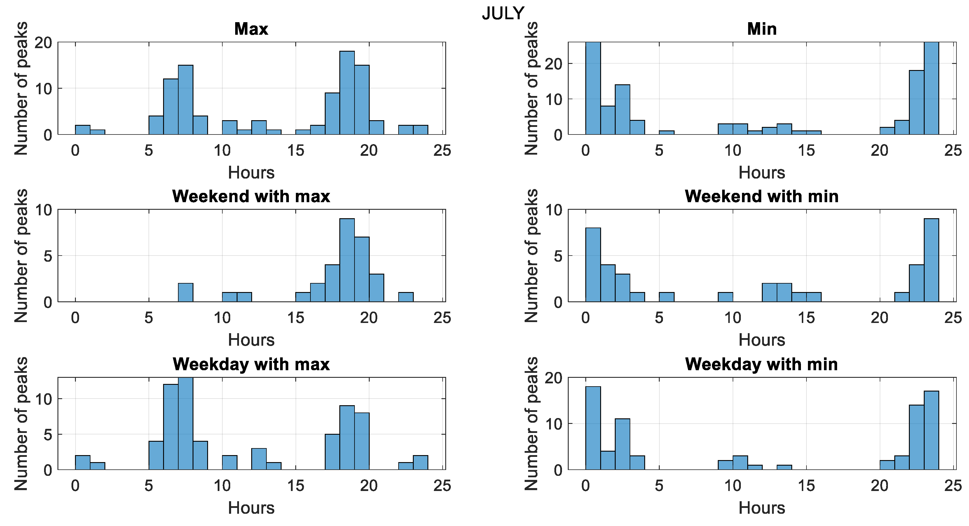
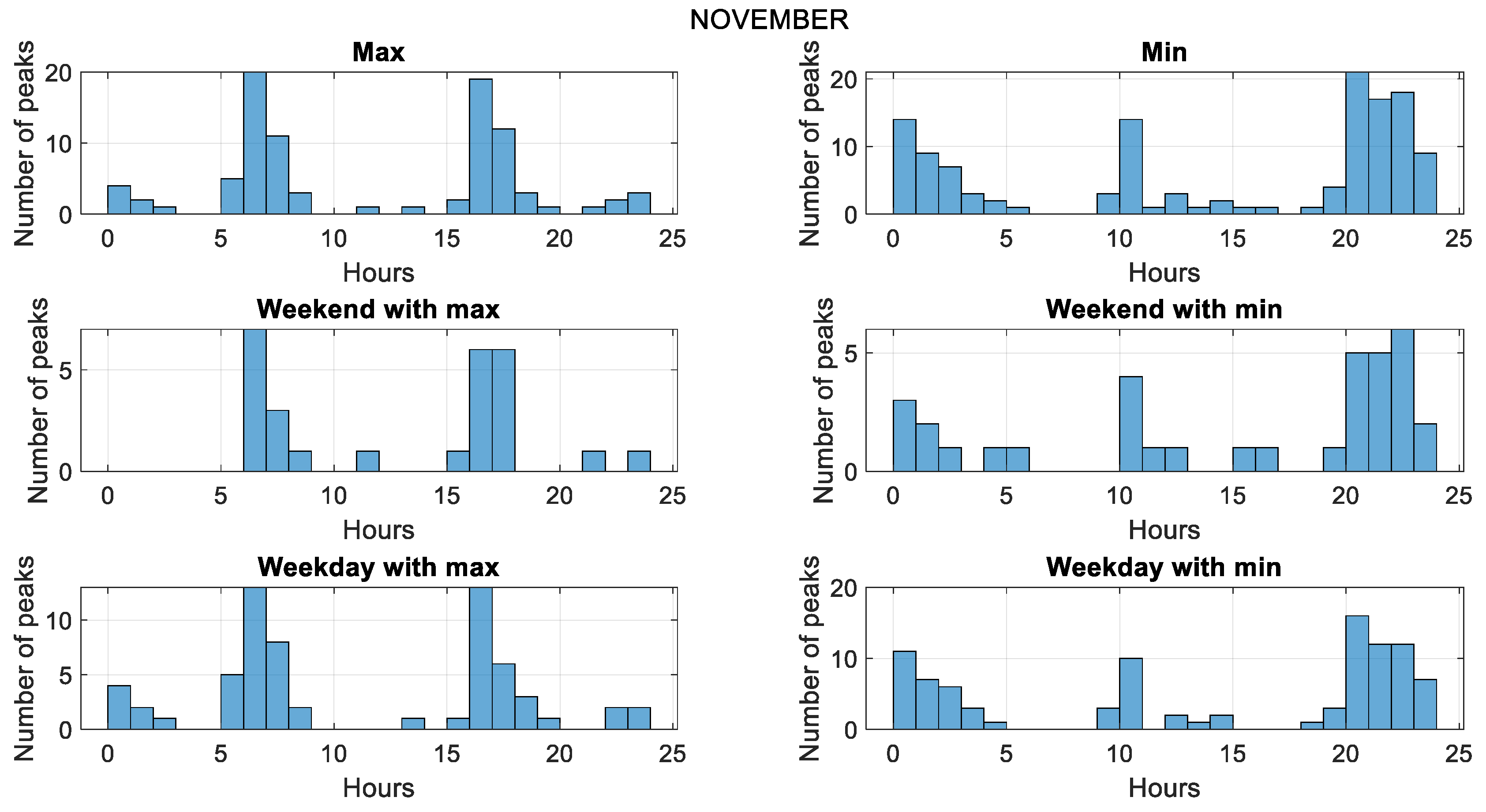
After collecting the local extrema, the data is represented through various graphs to facilitate comprehension and observation. First, we look at histograms differentiating between local maxima and minima, classified by whole month, weekdays, and weekends, to see if there are any different patterns in these time intervals throughout the month.

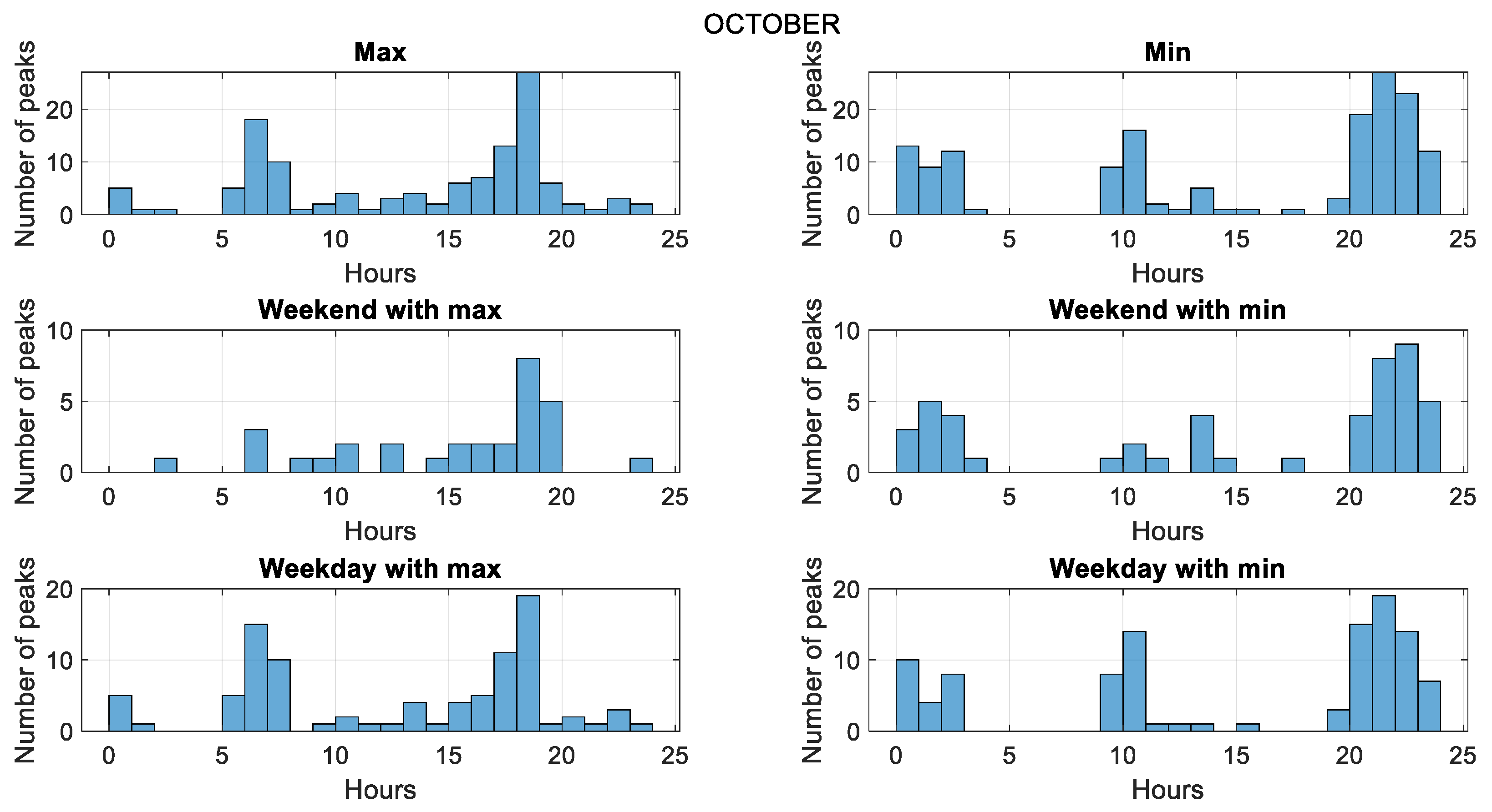
In Figure 6, the classification of the extrema identified with the algorithm is observed for both the whole month (July) and weekdays/weekends. Throughout the month, the extrema occur within a specific time period; in the case of local minima, between 9 p.m. and 4 a.m. We will look at other months to compare this observation. November and October are represented in Figure 7 and Figure 8 respectively:

We can see that the trend of the occurrence of the extrema is the same in both months.

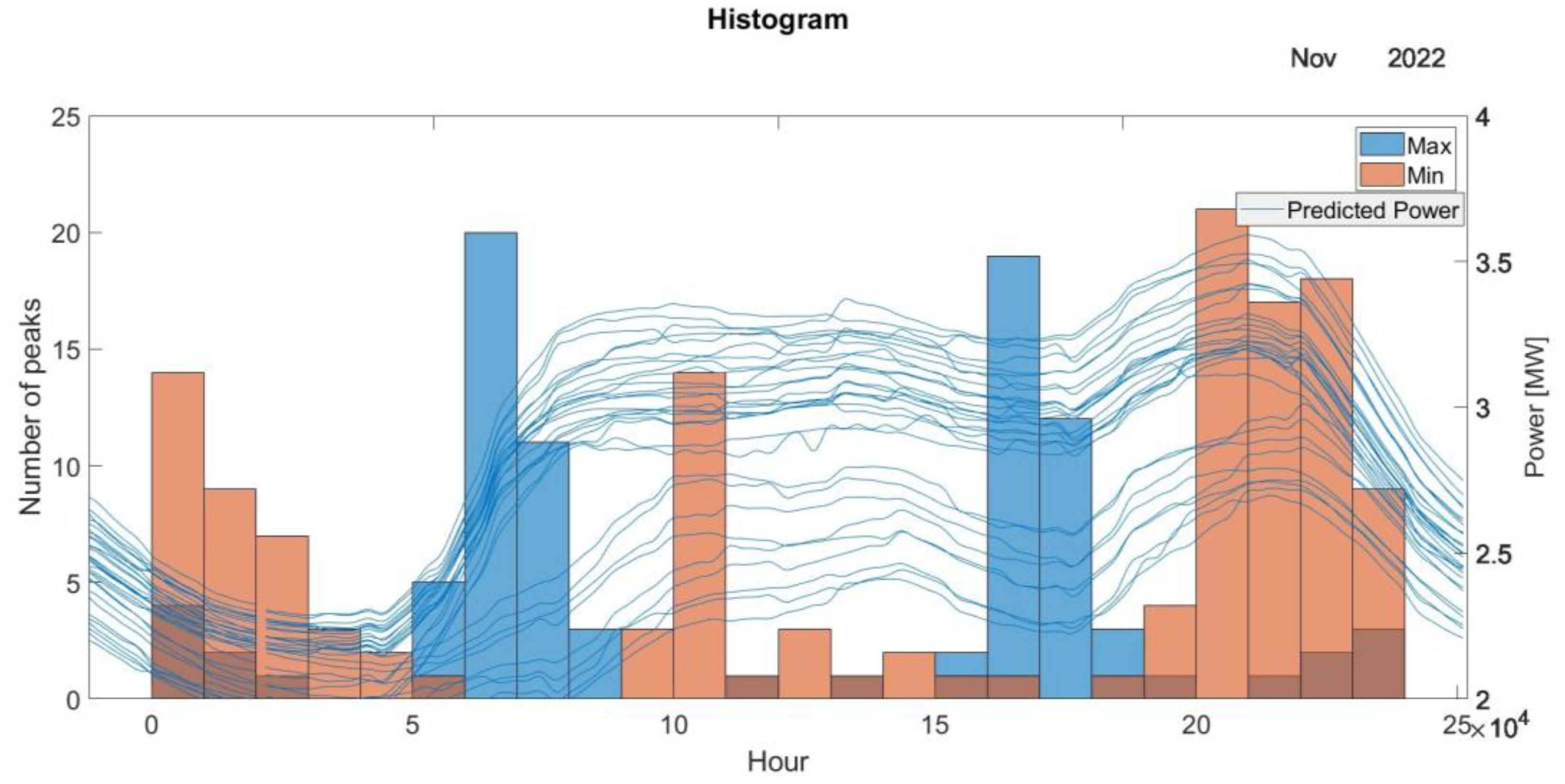
As the points identified by the algorithm fall within a specific time period, the next step is to relate these extrema to the grid energy sources. For this purpose, the above histogram is represented on the same graph as the forecasted power curve for November 2022.

In Figure 9, we observe the relationship between the localized minimum points and the downward trend of the predicted power gradient, while no relationship is observed between the detected maximum points and the upward trend of the predicted power. In order to look for any pattern that relates the maximum and minimum points localized by the algorithm, in Figure 10, we represent the points along with various renewable sources (wind power, PV solar, thermal solar, and hydropower) along with the maximum and minimum points represented by the symbols ‘o’ and ‘x’, respectively.

As shown in Figure 10, we can observe at a glance that no energy source has a relationship with the localized points except for two: hydropower and combined-cycle. In both cases, we notice a higher probability for localized maximum points to appear when there is an upward trend of power, and localized minimum points in sections with a downward trend of power. This effect is even more noticeable with hydropower, so we are going to focus the rest of the paper on this exact energy source.

Note that, in Figure 10, we are also considering the negative part of the power. This is due to some energy sources, such as solar thermal consuming power instead of generating it over certain time spans due to the automatic regulation system of the grid.

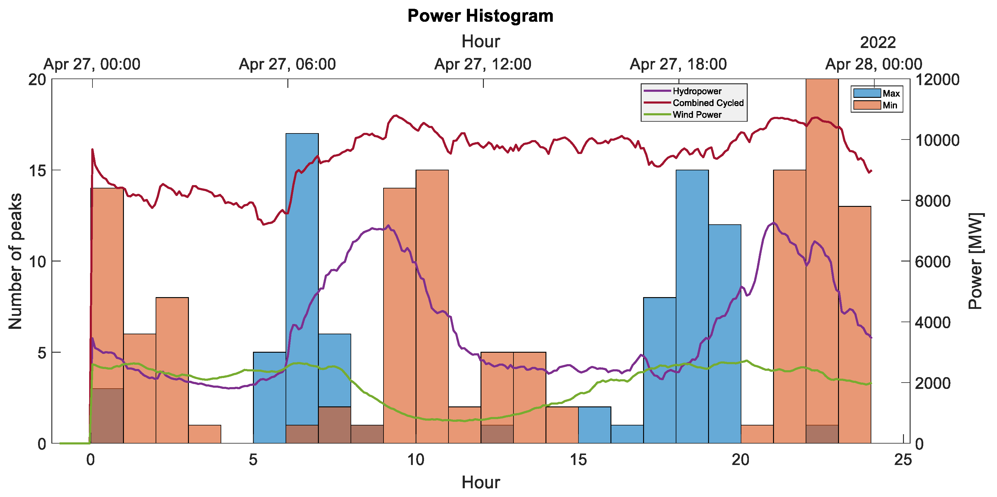
If we acquire the hydropower, combined-cycle, and wind power information from Figure 10 and represent it with a histogram for any given month as shown in Figure 7, we obtain Figure 11.

In Figure 11, we observe in greater detail the aforementioned assertion. We can observe that when the hydropower power curve tends to decrease, localized minimum points appear (orange bars), and when it tends to increase, localized maximum points appear (blue bars).

For combined-cycle, the same affirmation can be made to a lesser extent, but for wind power, no correlation between the power curve and the extrema has been found.

Later in this paper, we will corroborate all these assertions statistically.

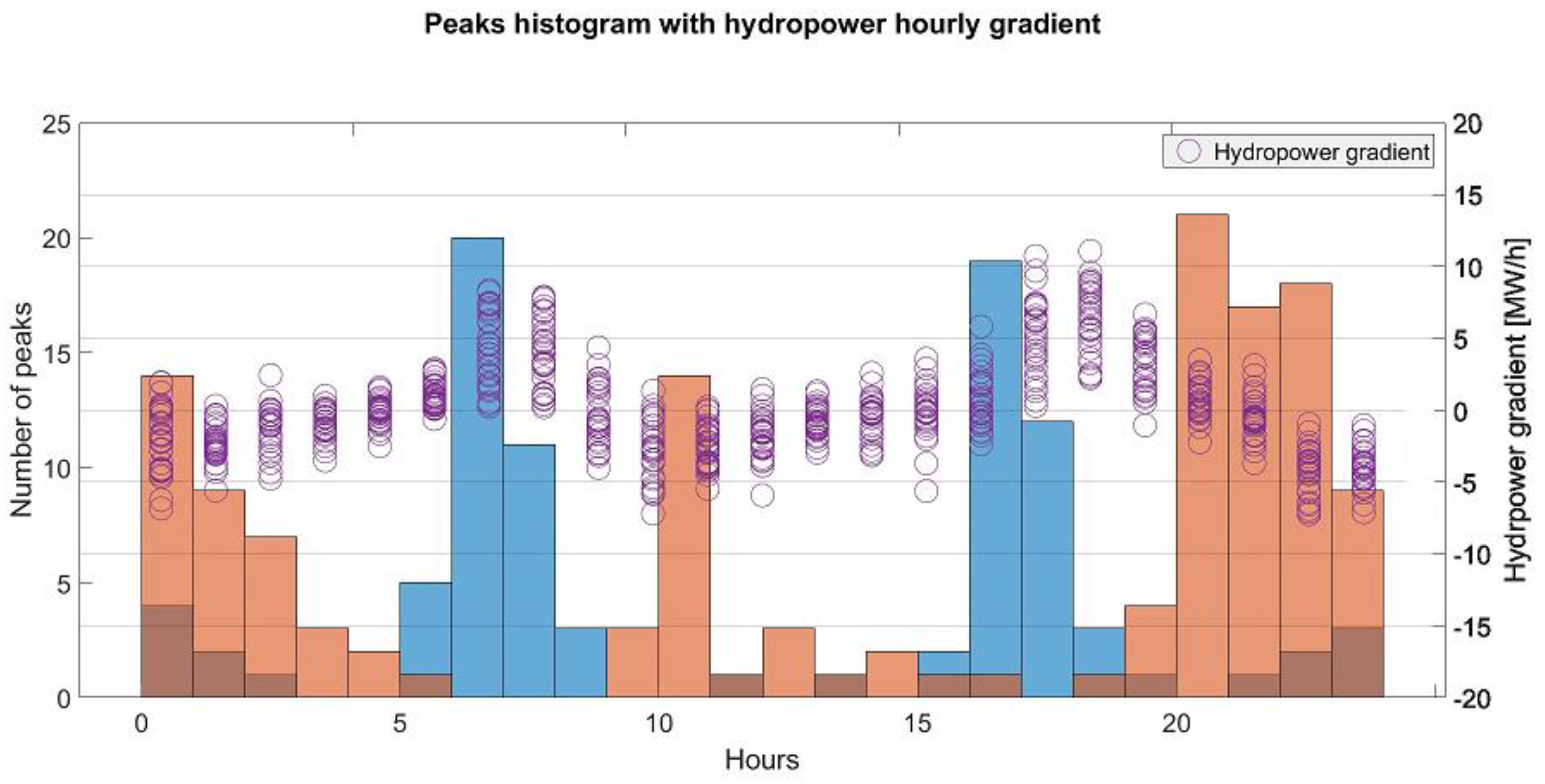
However, this representation shows only one day of power. If we calculate the hourly gradients only for the hydropower curve and represent the values of these gradients on a single histogram, we obtain the following representation.

In Figure 12, we can clearly notice that when localized minimum points appear, the slopes at which these minimum points occurr tend to be negative for the most part, representing a downward trend of the power curve. On the contrary, if we look at the areas of local maxima, we see that most of the gradients are positive, which represents the upward trend of the hydropower curve.

Table 1. Sign similarity percentage between pseudo-linear and linear regression.

Month	Sign Similarity Accuracy Percentage (%)
April	98.88
May	99.46
June	97.63
July	97.58
August	98.92
September	99.16
October	98.25
November	97.50
December	97.84
Average	98.36

shows the percentage of sign similarity of the gradients calculated using the pseudo-linear and linear regression methods. This indicates that both methods have a very high percentage of similarity in terms of the upward and downward trends, which are the focus of Figure 12.

It is important to note that the scale of hydropower gradient in Figure 12 is 1:50 to allow for a better representation of the data.

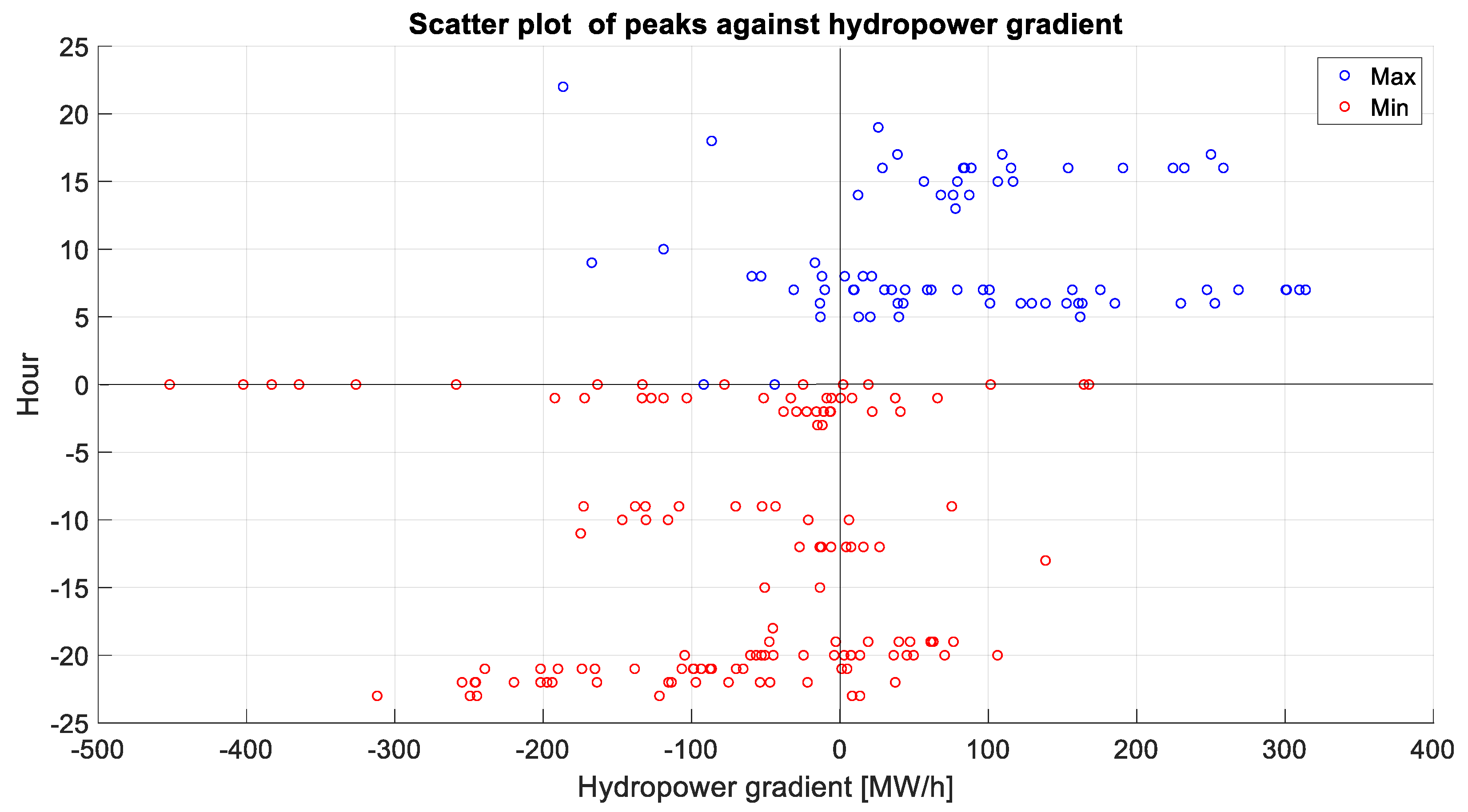
Finally, a scatter plot was created to confirm the veracity of the relationship between the hydropower gradient and the locations of the maximum and minimum points.

In Figure 13, we represent the values of the hourly slopes of the hydropower on the X-axis and, on the Y-axis, the hours at which these maxima or minima have occurred. Positive values on the Y-axis represent the hours where maxima have occurred, and negative values represent the hours where minima have occurred. Therefore, we see that quadrants 1 and 3 of the diagram contain the most localized points. Quadrant one indicates positive gradient values and local maxima obtained by the algorithms, while quadrant three indicates negative gradient values and local minima filtered by the algorithm.

Table 2. Accuracy percentage of maxima and minima with their respective gradient signs for hydropower.

Month	Maxima with Positive Gradient Accuracy Percentage (%)	Minima with Negative Gradient Accuracy Percentage (%)
April	89.65	89.59
May	90.97	87.77
June	73.63	85.48
July	74.48	81.89
August	71.42	87.50
September	85.71	92.15
October	73.39	81.82
November	83.52	84.10
December	82.67	78.46
Average	80.60	85.42

shows the percentage of local maxima and minima found in the first and third quadrants, respectively, as seen in Figure 13.

These statistical results support the hypothesis that local frequency maxima are correlated with the positive gradient of the hydropower, while local frequency minima are correlated with the negative gradient of the power.

In

Table 3. Accuracy percentage of maxima and minima with their respective gradient signs for combined-cycle power.

Month	Maxima with Positive Gradient Accuracy Percentage (%)	Minima with Negative Gradient Accuracy Percentage (%)
April	83.00	78.61
May	88.19	79.44
June	71.81	75.80
July	76.53	84.48
August	71.42	87.50
September	82.85	88.23
October	72.58	88.31
November	80.22	81.82
December	81.33	70.00
Average	78.66	81.57

and

Table 4. Accuracy percentage of maxima and minima with their respective gradient signs for wind power.

Month	Maxima with Positive Gradient Accuracy Percentage (%)	Minima with Negative Gradient Accuracy Percentage (%)
April	45.00	54.33
May	56.25	57.78
June	47.27	61.29
July	53.06	59.48
August	71.42	64.58
September	58.50	62.74
October	46.77	52.59
November	38.46	40.15
December	52.00	51.53
Average	52.08	56.05

, we can observe the accuracy percentage of matching maxima and minima with positive and negative gradients for combined-cycle and wind power respectively.

These results lead us to the conclusion that hydropower has the strongest relationship with the maximum and minimum values: the positive gradient of hydropower is correlated with a higher chance to detect a maximum, while the negative gradient is correlated with a minima appearance. Nonetheless, as mentioned earlier, the gradients of power from combined-cycle have a significant correlation with the extrema that cannot be ignored. However, in the case of wind power, no statistically significant correlation has been found with the extrema.

This paper has shown that hydroelectric power affects the frequency of the network more than the rest of the energy resources, mainly due to its impulsive nature, but its degree of affectation falls within the margins contemplated by the UNE-EN 50160:2011 standard for synchronized networks. The rest of the energy resources do not significantly affect the rate of change in frequency. The resilience of the network is therefore demonstrated. In real practice, this is achieved thanks to the introduction of automatic regulation techniques and procedures that are not the subject of this paper but are discussed hereinafter in order to establish the necessary link between cause and effect. These new tools and control solutions facilitate the integration and greater penetration of renewable sources without implying a reduction in the capacities of the electrical system in terms of stability and response to eventualities. They are based on advanced electrical systems that use the machine’s own inertia, effectively integrating the renewable resource into the frequency control of the electrical system.

The present research has shown that the stability of critical parameters, such as frequency, before the introduction of renewable sources as a response to sudden demands is currently guaranteed. The adaptation of new tools and solutions facilitates the integration of renewable sources without implying a reduction in the capacities of the system electricity in terms of stability and response to contingencies. This fact enables the large-scale introduction of renewable resources.

4. Discussion

The study reveals a strong correlation between the gradient of hydropower and the frequency variations of the Spanish electric grid; however, due to design limitations and unmeasured factors, a causal relationship between these two variables cannot be demonstrated. Therefore, caution is important when interpreting these results, and further research is needed to determine whether the observed correlation is due to a causal relationship or other factors that have not been considered in this study.

The main reason for this correlation could be attributed to the ability of hydropower plants to introduce large amounts of energy into the electricity grid in a relatively short period of time. Since the frequency of the electricity grid is directly proportional to the amount of energy supplied and consumed, sudden changes in hydropower could have a significant impact on the grid frequency.

It is important to note that abrupt frequency variations in the electricity grid can have a negative impact on the country’s industrial equipment. This is because electrical equipment is designed to operate within specific frequency and voltage limits, and variations outside these limits can cause mechanical stress and strain that can damage internal components and reduce equipment efficiency [2].

Therefore, it is essential to implement ad hoc measures to control the frequency and voltage of the electricity grid and minimize abrupt variations while maintaining the stability and quality of the supplied electrical energy. In addition, it is essential that industrial equipment be designed to withstand frequency and voltage variations within established limits to avoid damage and loss of efficiency.

Finally, it should be noted that despite the limitations of this study, the results provide a solid foundation for future research seeking to determine causality between grid frequency and hydropower. It is necessary to carry out studies that use more rigorous and comprehensive methods, such as obtaining frequency data at a point near a hydropower plant, as frequency disturbances will be measured more clearly at points closer to the source of the disturbance than at points farther away.

The results of such investigations are useful for grid operators in the development of strategies related to the implementation of renewable energy resources in the grid.