Nonintrusive Load Monitoring Using Recurrent Neural Networks with Occupants Location Information in Residential Buildings

Abstract

Nonintrusive load monitoring (NILM) is a process that disaggregates individual energy consumption based on the total energy consumption. In this study, an energy disaggregation model was developed and verified using an algorithm based on a recurrent neural network (RNN). It also aimed to evaluate the utility of the occupant location information, which is nonelectrical information. This study developed energy disaggregation models with RNN-based long short-term memory (LSTM) and gated recurrent unit (GRU). The performance of the suggested models was evaluated with a conventional method that uses the factorial hidden Markov model. As a result, when developing the GRU disaggregation model based on an RNN, the energy disaggregation performance improved in accuracy, F1-score, mean absolute error (MAE), and root mean square error (RMSE). In addition, when the location information of the occupants was used, the suggested model showed improved performance and good agreement with the real power and electricity consumption by each appliance.

1. Introduction

As energy consumption increases worldwide, so does the demand for energy management. In addition, as the demand for appliances and personal equipment increases due to the increase in population and living standards, electricity use in the building sector is also increasing [1]. In South Korea, about 39% of electricity consumption as of 2018 occurred in residential and commercial buildings, and the rate is increasing by about 1% every year [2]. Accordingly, there is an increasing need to reduce the electricity consumption in the residential and commercial building sectors.

Among the various measures for energy saving, energy disaggregation, also called nonintrusive load monitoring (NILM), is the process of estimating individual loads of facility systems by using the total electric power consumption measured by a household power monitor [3]. In other words, energy disaggregation investigates detailed information on appliance-specific or usage-specific energy consumption from the total energy usage. According to Darby, when the energy disaggregated results were posted for users, the energy use efficiency improved by about 15%, and 81% of users answered that the information was useful [4]. Therefore, this energy disaggregation shows the user that it is more effective to save energy by posting the power usage per appliance rather than the total power usage.

This energy disaggregation is a process of power consumption analysis based on the data collected in a timed sequence, as shown in Figure 1. The most widely used algorithm for learning probabilistic models of time series data is the hidden Markov model (HMM) [5] and the factorial HMM (FHMM). The Markov process and its variant algorithms are generally used for energy disaggregation [6]. However, recent studies have introduced algorithms using machine learning (ML) technologies for energy disaggregation in buildings.

NILM can be divided into event-based or state-based approaches. Event-based approaches try to capture statistically significant variations of the signals. On the other hand, state-based approaches use appliance load distribution models to disaggregate the total power. Hidden Markov models (HMM) and combinatorial optimization (CO) are commonly used methods for state-based approaches. Integer programming (IP) can also be used to disaggregate without supervised learning [7,8].

As described above, NILM is a process of analyzing energy use at home or in buildings, and this energy use is related to the activities of the occupants. Accordingly, several studies have been conducted on energy use analysis based on occupant behavior in various types of buildings [9,10,11]. Additionally, the application of nonelectrical data is important as nonelectrical features such as occupancy and indoor/outdoor temperature information help improve the performance of energy disaggregation models [12].

Conventional energy disaggregation models with FHMM have limitations. According to Kim et al. [6] and Holmegaard and Kjærgaard [13], when energy disaggregation is performed using the FHMM, the disaggregation performance decreases as the number of home appliances increases. FHMM also limits the pattern recognition of multistate appliances or appliances with similar power consumption. To overcome these limitations, machine learning technologies can be used such as recurrent neural networks (RNN). The RNN is a dynamic system that efficiently uses time information [14]. For this reason, it is widely used for processing time series data analysis. It is also useful to process many input and output variables as a deep learning algorithm based on a neural network. Disaggregation with RNN can be robust to classify various appliances and the prediction of power consumption in buildings. Thus, this study introduced an algorithm based on a RNN to compensate for the limitations of FHMM in energy disaggregation.

In addition, this study incorporated occupant location information as nonelectric information in NILM to improve performance. Most home appliances including fridges, TV, washers, and dryers are in a fixed location. Therefore, it can be thought that the occupant location is closely related to the operation of the appliance in the case of appliances interacting with the user (e.g., TV, PC, etc.), or home appliances operated by the occupants’ contact (e.g., lighting switch, a fridge, a microwave range, etc.). Accordingly, by analyzing the energy disaggregation performance when using the information on occupant location, the performance of the NILM can be improved. In recent years, in a smart home environment, the need to monitor infants and children as well as the elderly is increasing, and households with cameras for home security are increasing. Therefore, in this study, we propose a method of utilizing an existing home security camera to detect the occupants’ location in a house. As a result, it does not require the installation of additional sensors to acquire the occupant location information.

2. Literature Review

2.1. Occupant Localization Approach

Occupant localization in the indoor environment has been studied in various research with different methodologies and purposes. Occupant localization is also related to occupancy detection in buildings, and is used for building energy management [15,16], managing space [17], and monitoring elderly people [18]. The information on the number and localization of occupants inside buildings could improve the energy efficiency with an IT network and a building automation control system while maintaining appropriate thermal comfort for the occupants [19].

In previous research, various methods have been proposed for occupant localization including RGB-D camera vision [20,21], floor vibration sensors [19,22], WiFi infrastructure [23,24], radio frequency identification [25], and so on. However, current methods require the installation and maintenance of additional sensors or display markers that assist with localization, which hinders the practical application in the field. In addition, tracking mobile devices or wearable devices in the built environment is suggested, but it is hard to keep asking the occupants to always carry their devices [26].

2.2. Nonintrusive Load Monitoring Approach

NILM is a low-cost approach to individual load monitoring and has been studied intensively in recent years [6]. The NILM results provide consumers or building managers with the opportunity to reduce their energy costs through real-time power consumption feedback. Load information from each device can be used by electricity companies, smart building controllers, home appliance manufacturers, and individual energy consumers to increase the energy efficiency [27].

In NILM, appliance features are mathematically characterized, and a data collection system is required to detect the features. There is a common principle that a mathematical algorithm detects individual features from the total electric power signal [28]. In general, the NILM approach can be divided into two approaches depending on the sampling rate of the hardware that records the power and voltage for energy measurements. The first approach is to use low-frequency hardware, and the second is to use higher-frequency sampling hardware [28].

The approach that utilizes low-frequency hardware is based on the changes in the real power and reactive power [29]. This method is based only on the changes in real power, thus disaggregating only devices with a relatively large load based on the data sampled over a long period [30]. The approach that utilizes higher-frequency sampling hardware not only includes power change, but also a method to utilize harmonics [31,32]. One of the conventional approaches for NILM is to use the factorial hidden Markov model.

2.2.1. Factorial Hidden Markov Model

As described above, it is possible to perform energy disaggregation with the FHMM, which combines Markov chains that represent the state of equipment over time [13]. FHMM is an extended HMM with a state space composed of a cross-product of state variables [5], as shown in Figure 2. There are N sequences of the hidden states, and the shape is the same as that of a stacked HMM [6]. In NILM, each sequence corresponds to one appliance.

Holmegaard and Kjaergaard [13] estimated the state of industrial equipment using FHMM. Batra et al. [33], Kim et al. [6], and Yue et al. [34] compared the performance of the matrix factorization method, long short-term memory (LSTM) model, and unsupervised NILM algorithm along with the FHMM as a baseline, respectively.

2.2.2. NILM with Nonelectric Information

In NILM, load signatures, which are characteristic of each appliance, can be classified into steady-state signatures, transient signatures, and nontraditional signatures. The steady-state signatures are load characteristics extracted when the device is in steady-state operation. Transient signatures appear in the period between the steady-state operation and the OFF state of the device [35]. Nontraditional signatures are features that have recently been increasingly used in energy disaggregation including nonelectric information [35,36].

According to Abubakar et al. [36], energy disaggregation can be conducted using nonelectrical information such as temperature, time of day, and start-up time as nontraditional signatures, and disaggregation performance can be improved when such information is added. In addition, using nonelectric information in NILM can help identify abnormal states in equipment operation such as peak consumption times, malfunctions, and low efficiency due to technological obsolescence [37].

Accordingly, Kim et al. [38] and Zeifman and Roth [39] investigated various nonelectric information including the ON and OFF duration distribution and the frequency of appliance usage that could be applied to improve the segmentation performance.

3. Methods

The suggested approach uses RNN-based algorithms along with the occupants’ localization information as nonelectric information. In order to make new models and test the performance of the developed model, we set up and collected data in a testbed.

3.1. Experimental Setting and Data Collection

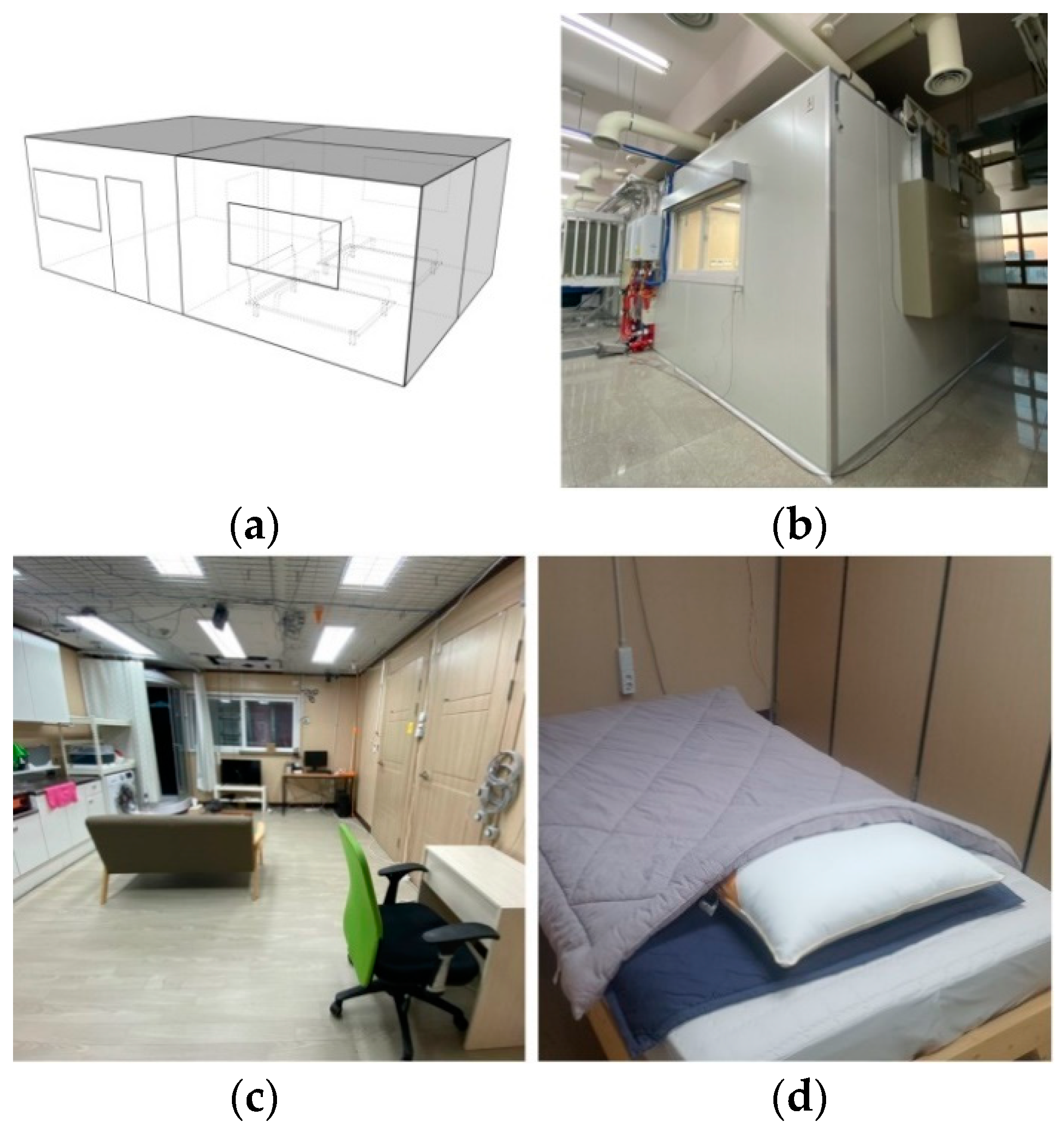
The data used in this study for NILM was collected from the Smart Living Testbed (SLT) at Dankook University, Yongin, Korea. The SLT was designed to collect indoor environment data under the control of various indoor climate control equipment used in residential and commercial buildings. The SLT is a rectangular chamber consisting of one living room and two bedrooms, as shown in Figure 3, and was equipped to monitor the energy consumption from each piece of equipment and the indoor environment data (e.g., temperature, relative humidity, CO₂ concentrations). These data were measured every minute. The SLT was equipped with basic facility systems including a VRF (variable refrigerant flow) system, a floor radiant heating system, an energy recovery ventilator, and a dimming system, and an additionally installed 14 household appliances, as shown in

Table 1. List of appliances in the SLT.

Number	Appliance
1	Desktop
2	Fridge
3	Air conditioner
4	Lights
5	Energy recovery ventilation (ERV)
6	Washer
7	Microwave
8	TV
9	Laptop
10	Rice cooker
11	Hot water mat
12	Hair dryer
13	Humidifier
14	Air cleaner

. Electric power was monitored for every piece of equipment for energy disaggregation along with the total electric power. In addition, a home security camera was installed on one side of the ceiling in the living room.

The data collection was performed for five days during a heating season. Two occupants, one female and one male, stayed in the living testbed. Each occupant lived in the same as their home for about 2.5 days in turn. We collected the data of the outlet-specific electric power (W) from each appliance and the indoor video data through a home security camera. Based on the collected power data for each appliance, the total power for the 14 appliances was added as a variable to construct a time series dataset to train and validate the electricity consumption disaggregation model.

The input data size of the NILM model was N × 1, and the output data size of the power (W) prediction model was N × 14 (power consumption of 14 electronic devices), while the output data size of the state estimation model was also N × 14 (state of 14 electronic devices). It was assumed that there was no noise represented by unknown loads.

In this experiment, it is necessary to collect indoor video data to understand the occupants’ behavior. Therefore, the participants spent most of their time in the living room where the camera was installed and only entered the bedroom when they needed to sleep.

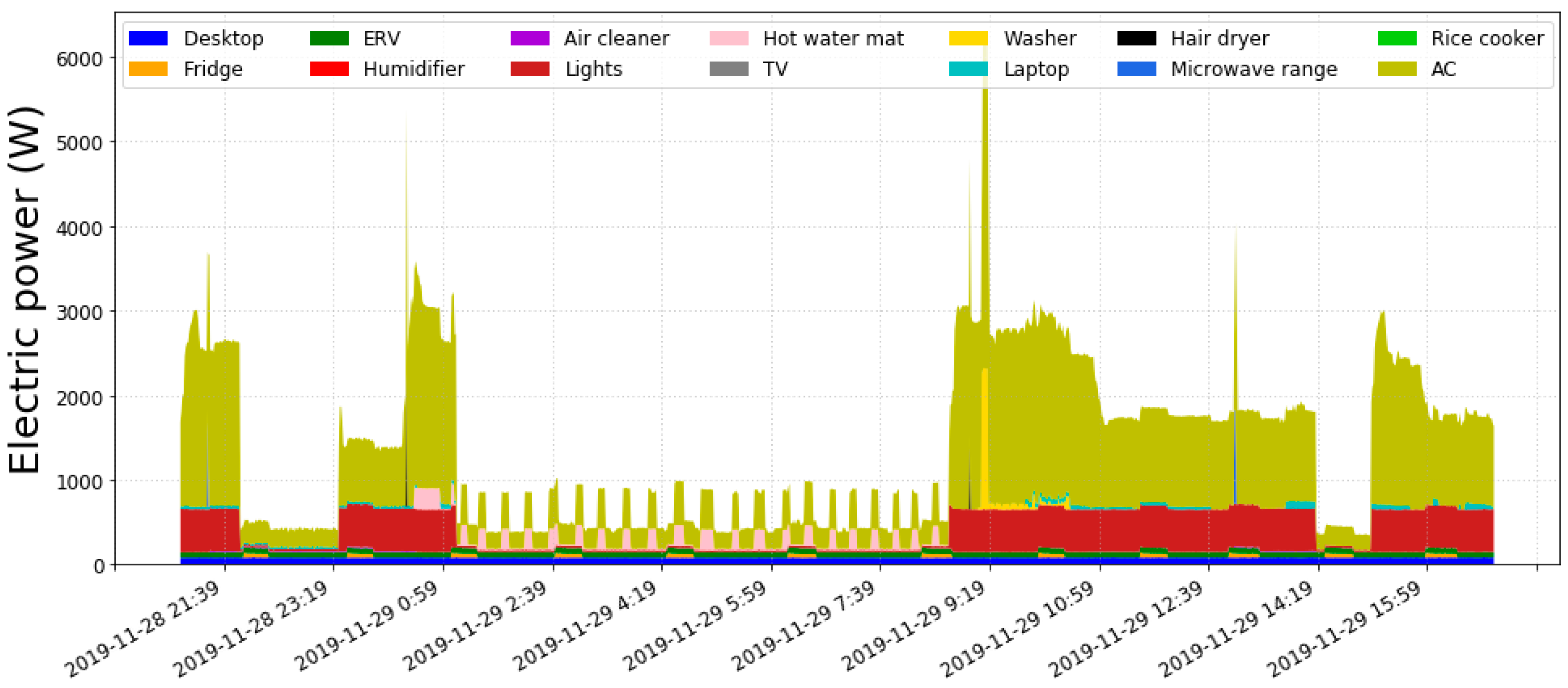
Based on the collected indoor video data, a dataframe type of occupant location dataset was constructed to be used as an input variable for an advanced energy disaggregation model. In this process, the image data were captured every second and converted to the time series occupants’ location data. Figure 4 shows an example of electric power data by 14 appliances from the Smart Living Testbed.

3.2. Recurrent Neural Networks

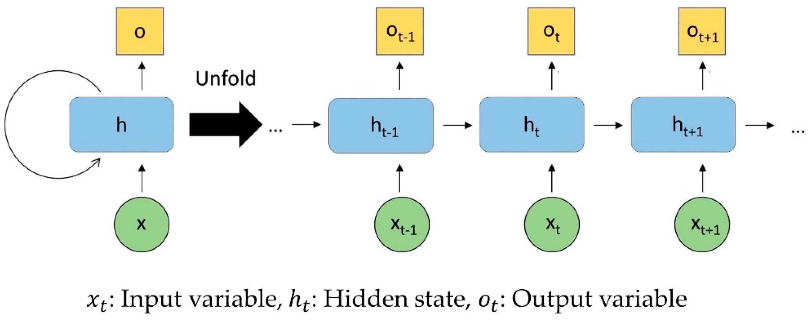
The suggested model uses RNNs to increase the performance of the energy disaggregation and the number of appliances for analysis. The recurrent neural network (RNN) is a neural network characterized by sending the result values at the hidden layer back to the input of the hidden layer, as opposed to the feed-forward neural network in which the computation process in the hidden layer is directed into the output layer. The addition of a time series concept to the general neural network has the advantage of storing previous information in a hidden layer, making it a suitable model for learning and sequentially predicting the structured time series data [40].

Figure 5 shows the structure of a recurrent neural network in which a memory cell is in the concealed layer that can store the previous values, and the task of sending the current and previous information, hidden state, to the hidden layer at the next point is repeated. As these procedures become longer and the internal structure becomes more complex, there is a limit due to the problem of the vanishing gradient. In addition, this repetition has a limitation in that the problem of long-term dependencies, in which historical information stored in the hidden layer, is not delivered to the end. More details can be found in [41].

3.2.1. Long Short-Term Memory

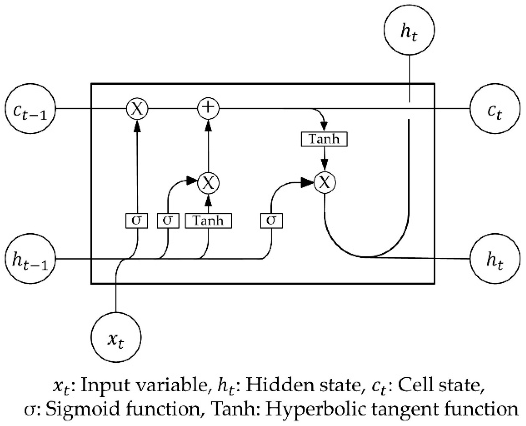
Long short-term memory (LSTM) is a variation of the RNN structure. It was designed to solve the problem of long-term dependencies, a chronic problem of RNN. LSTM, like a typical RNN, is suitable for learning and predicting the time series data. A LSTM unit is composed of a cell state, an input gate, an output gate, and a forget gate, as shown in Figure 6. The input gate determines whether new information is stored in the cell state. The forget gate consists of a sigmoid function and determines what information is removed from the earlier cell state. The output gate then derives the final output value. The detailed architecture and explanation can be found in [42].

3.2.2. Gated Recurrent Units

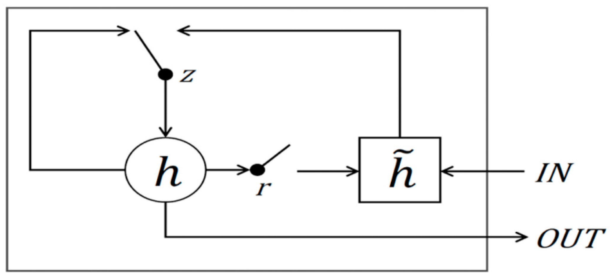
A gated recurrent unit (GRU), proposed by Cho et al., is a strain algorithm that complements the shortcomings of a basic RNN [43]. The GRU consists of a relatively simpler structure than the LSTM. The LSTM consists of a total of three gates (i.e., the forget gate, the input gate, and the output gate), while the GRU consists of two gates (reset gate:r and update gate:z), where the role of the port gate is divided into the remaining two gates, as shown in Figure 7. These gates are vectors that determine the information to forward. The reset gate decides how to combine the previous memory with the new input value, and the update gate determines how much of the previous memory is to be delivered.

3.3. Occupant Localization Based on Image Data

The suggested NILM approach uses the occupants’ location information to enhance the performance of the RNN-based model. Localization was achieved by using CNN in this study.

3.3.1. Convolution Neural Networks

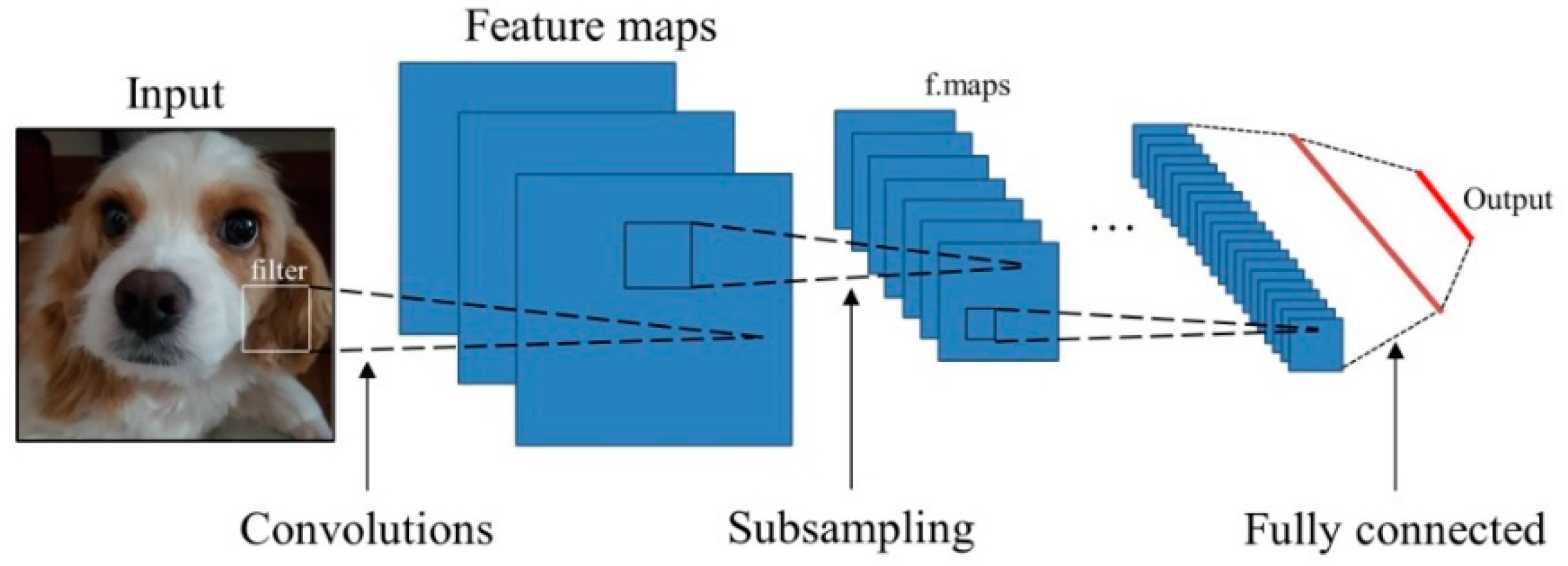
A convolution neural network (CNN) is a class of deep neural networks most commonly applied to visual image analysis. A CNN is composed of the input and output layers and several hidden layers like normal neural network algorithms [44]. The hidden layers of CNN are composed of convolutional layers, pooling layers, and a fully connected layer. The convolutional layer has a convolution filter and a nonlinear activation function. The convolution filter is a common parameter to find the features of the input data. This is usually composed of a square matrix and creates a feature map through the convolution operation. After the convolution operation, a nonlinear activation function is applied to the feature map [45]. In the pooling layer, the dimension of the feature map is reduced, and the noise of the input data can be decreased by this operation. After the pooling operation, all feature map values are connected to the input nodes of the fully connected layer [45], as shown in Figure 8. CNNs with these characteristics are used in various fields including image recognition and classification and natural language processing.

3.3.2. Occupant Detection and Image Processing

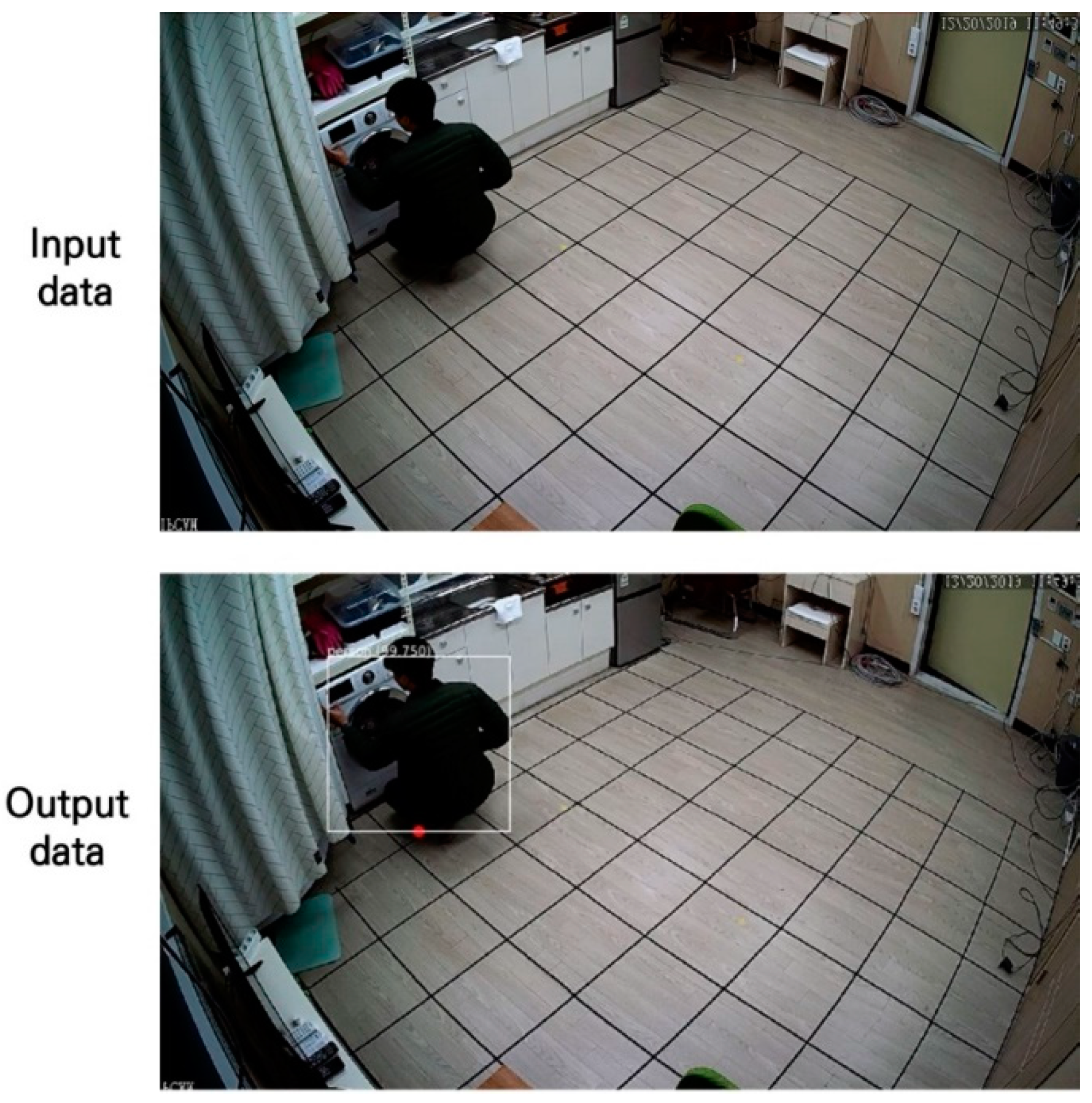
In this paper, the object detection model YOLOv3 [46] was used for the detection of occupants through the image data. The YOLOv3 is the most widely used deep learning-based object detection model and can detect various objects including humans and animals using a single feed-forward convolution neural network. In this study, the location was estimated by detecting occupants, so the code was modified for the YOLOv3 model to only detect humans. When a human is detected in the image data, a transparent bounding box is created around the person and a specific RGB value point is displayed in the lower center of the bounding box. The RGB value was used for the pointing process. Figure 9 shows the input images and output images of occupant detection and the pointing processes. The bounding box was originally transparent; however, for reference, it is marked in white in the figure with a red dot.

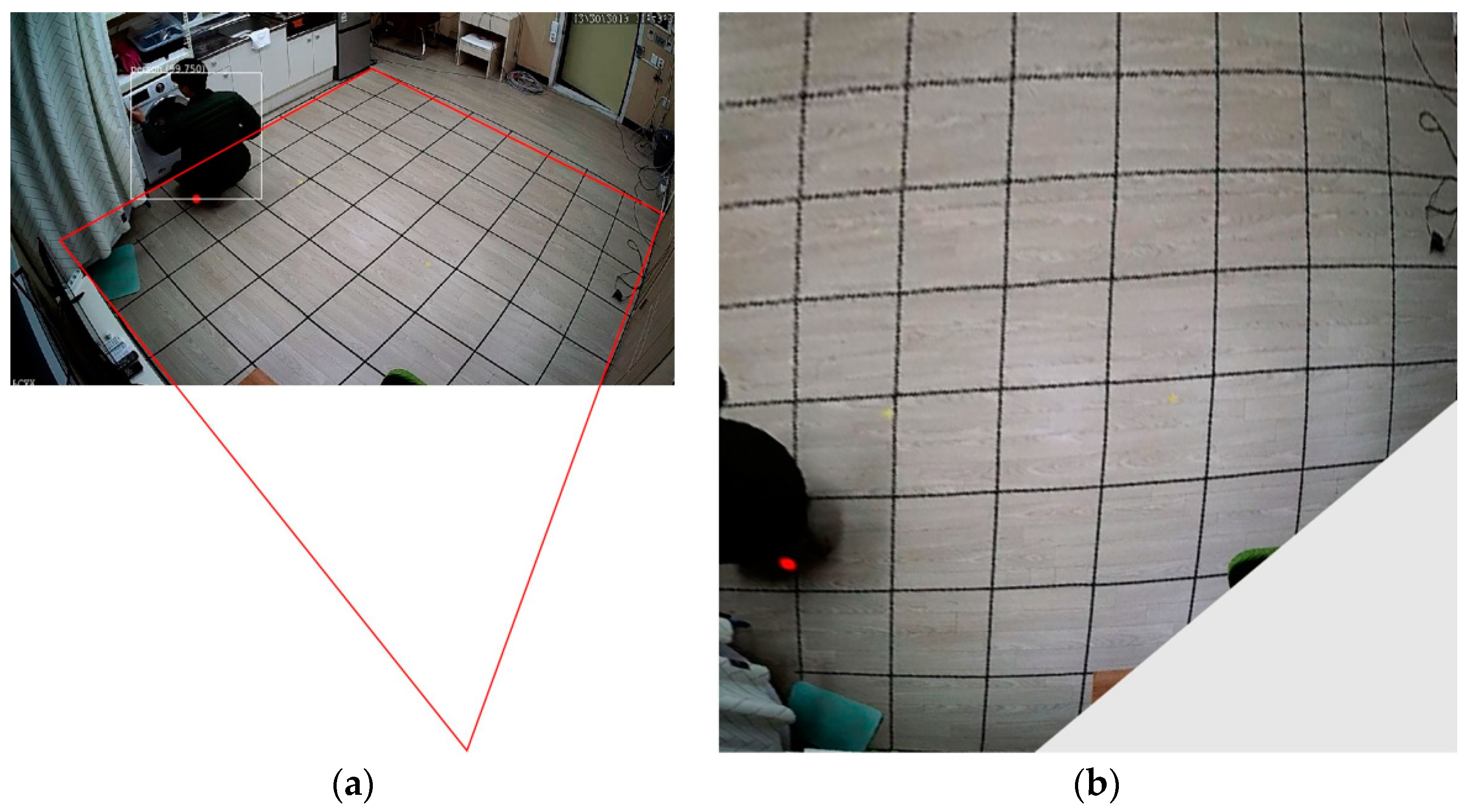
In addition, a process of perspective transformation of the image was performed using OpenCV (Open Source Computer Vision). OpenCV is a programming open source developed by Intel for real-time computer vision. A point from the output image in Figure 9 was used to estimate the location of an occupant. Therefore, it is necessary to perform perspective transformation and planarization based on the bottom surface of the output image. As the perspective transformation is based on four vertices, it is necessary to designate the vertices of the floor surface. In the case of images used in this study, there was a limitation that all floor surfaces in the living room were invisible due to the camera angle. Therefore, the perspective transformation was performed by estimating the position of one vertex based on the grid on the floor. Figure 10 is an example of the result of this perspective transformation.

Through RGB extraction, the pointed part was converted into coordinates to create the occupant’s location coordinates. The example is shown in Figure 11.

In this study, as the occupant’s location data were used as an input variable of the RNN, the task of making the time series data in units of 1 min was processed as with other input variables in the energy disaggregation model. After the distance between each appliance was calculated based on the occupant’s location coordinates, the smallest value among the distances between each device and the occupant for 60 s was selected and arranged as a representative value to convert the interval of the corresponding distance data from 1 s to 1 min. The distance dataset in units of 1 min were variables containing the location information of the occupant; these variables were used as the input variables of the energy disaggregation model.

4. Results and Discussion

4.1. Experimental Cases

In this study, we suggested a new NILM approach that used a RNN with occupant location information as the input variables. We developed a power disaggregation model and a state estimation model separately by using the data from 14 appliances. To evaluate the performance of the suggested method, experimental cases were designed as follows.

First, the performance could be compared for the electricity consumption disaggregation and appliance state estimation with the existing FHMM. Therefore, one FHMM and two RNN models (LSTM and GRU, respectively) were developed to evaluate the performance of the disaggregation models and the state estimation models, respectively.

Second, in the case of evaluating the usability of the occupant location information, the superior model was selected based on the result of the performance comparison between two RNN models (LSTM and GRU). The performance improvement of the selected models with or without the occupant location information was evaluated based on the performance metrics.

4.2. Performance Metrics

The electricity consumption disaggregation performance of the suggested energy disaggregation model was evaluated with error metrics such as the MAE and root mean square error (RMSE). Each metric was expressed as the following equation (Equations (1) and (2)). The MAE and the RMSE are indices that indicate the error between the actual value and the estimated value through the predictive model, which have been widely used for model performance verification [47]. The MAE is less sensitive to errors with large absolute values than the RMSE. The RMSE is more suitable for representing the model performance than the MAE when the error distribution is expected to be Gaussian [48]. Although the two error metrics are similar to each other, it is appropriate to present both to evaluate the performance of the model in various ways [49].

$$MAE={\sum }_{i=1}^n\left|Y_{Actual,i}-Y_{model,i}\right|/n$$

(1)

$$RMSE=\sqrt{{\sum }_{i=1}^n{(Y_{Actual,i}-Y_{model,i})}^2/n}$$

(2)

$Y_{Actual,i}$: Actual value, $Y_{model,i}$: Predicted value, $n$: Number of samples.

In the case of the appliance state estimation, the performance of the model is expressed as a confusion matrix that is frequently used in classification performance analysis. In addition, we also evaluated the accuracy and F1-score with a range of 0.0–1.0 (Equations (3) and (4)).

$$Accuracy=\frac{TP+TN}{TP+TN+FP+FN}$$

(3)

$$F1-score=2\ast \frac{\frac{TP}{TP+FP}\ast \frac{TP}{TP+FN}}{\frac{TP}{TP+FP}+\frac{TP}{TP+FN}}$$

(4)

$TP$: True Positive, $FN$: False Negative, $FP$: False Positive, $TN$: True Negative.

4.3. Design of Energy Disaggregation Model

This section describes the design process of a model for energy disaggregation. In the model design, all processes were carried out using Keras 2.2.4 version as a framework, that is, the overall structure of the model in the Python 3.7.3 environment, and Tensorflow-gpu version 1.14.0, a deep learning open source package, was used as the back end.

For the FHMM-based energy disaggregation model, the FHMM model of the NILMTK package [50], a Python-based open-source toolkit, was used. In the case of the RNN-based energy disaggregation model, the LSTM and GRU models were used as described in Section 4.1.

In this study, holdout validation was used for model training and validation. Holdout validation is a simple cross-validation for overfitting prevention and generalization of the model by splitting the entire dataset into the training dataset to be used for model learning, and the test data to be used for validation and performance testing [51]. In this study, the datasets collected for learning the energy disaggregation model were split into training data and test data in time series order. As shown in

Table 2. Dataset structure for learning and validation.

Dataset	Period	Proportion
Training data	2019.11.25 09:39:00~2019.11.28 09:59:00	70% (4341 rows)
Test data	2019.11.28 10:00:00~2019.11.29 17:00:00	30% (1861 rows)

, the training data consisted of about 70% of the entire dataset, 4341 rows, and the test data consisted of about 30% of 1861 rows.

4.4. Optimization of Hyper-Parameters

This section describes the hyper-parameter adjustment of the energy disaggregation model based on RNN. Hyper-parameters are values that are adjusted by the user in the model training process. The proper selection of hyper-parameters is an important task in improving the performance of the model. In general, the optimization of these hyper-parameters is based on grid search and random search. Grid search is a method of organizing each set of hyper-parameters to be adjusted into an appropriate finite set and considering the number of all cases of each finite set. The final selection of each hyper-parameter is made by an indicator measuring the model performance, and the range of finite sets is reasonably defined by the user [52]. In this study, the hyper-parameters of the model were optimized using the grid search method. In the GRU model, the number of hidden layers was set to 3, the hidden nodes were set to 64, and the batch size was set to 64. The activation function of the hidden layer was set to the rectified linear unit (ReLU) or exponential linear units (ELUs). Adaptive moment estimation (ADAM) was used as the optimizer. mean squared error (MSE) was used as a loss function to determine the degree of learning, as shown in

Table 3. Hyper-parameters of the RNN models.

Hidden Layers	Hidden Nodes	Batch Size	Activation Function	Optimizer	Epoch
3	64, 64, 64	64	RELU and ELU	ADAM	200

. In addition, the early stopping method was used to prevent the model from overfitting and to use the weight at the point where the verification loss was the smallest. This hyperparameter was applied equally to both the LSTM and GRU, the RNNs used in this study.

4.5. Results

4.5.1. Performance of Electricity Consumption Disaggregation

In this section, we compare the performance of NILM based on the FHMM, and two RNN algorithms (LSTM and GRU). The performance when the same test dataset was applied was compared, and the input and output variables were also the same. The input variable of the three energy disaggregation models was the total power (W), and the output variable was the power (W) of 14 appliances.

Performance evaluation of the electricity consumption disaggregation was based on the result of disaggregating the electricity consumption (kWh) of each device from the total electricity consumption (kWh) and the error metrics of disaggregating the electric power (W) per minute by each appliance.

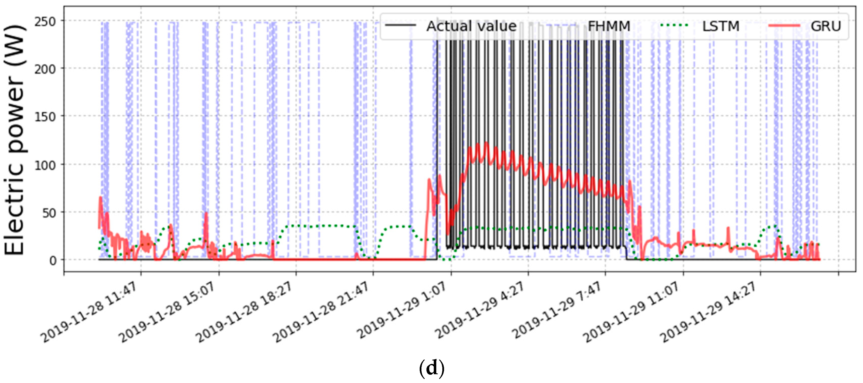
Figure 12 shows the electric power disaggregation results from three algorithms for four representative devices (air conditioner, lights, laptop, and hot water mat). As can be seen from the graph, since the FHMM-based disaggregation model has a characteristic of inferring the electric power (W) at the time of operation with a specific value, it tends to show a rectangular pattern. Therefore, in the case of an appliance such as the lights in Figure 12b, it is advantageous to infer the electric power consumption. However, in the case of a multistate appliance such as an air conditioner in Figure 12a, the inferred accuracy from FHMM is very poor. In contrast, the RNN-based disaggregation model (LSTM and GRU) can learn the electric power patterns that change over time, thus showing better performance for the electric power relatively well compared to the FHMM.

Table 4. Results of the electricity consumption (kWh) disaggregation by appliance.

Appliances	Actual Value (kWh)	FHMM (kWh)	LSTM (kWh)	GRU (kWh)
Air conditioner	27.96	9.90	15.43	19.66
Lights	9.12	8.16	12.69	14.50
Desktop	2.52	2.19	2.18	2.59
ERV	2.03	0.87	2.01	1.81
Hot water mat	0.81	3.57	0.64	0.92
Laptop	0.46	0.53	0.51	0.57
Fridge	0.40	0.71	0.44	0.46
Washer	0.27	12.72	1.15	0.90
Air cleaner	0.27	0.16	0.01	0.24
Rice cooker	0.08	3.79	0.11	0.35
Microwave	0.07	0.06	0.68	0.24
Hair dryer	0.04	0.19	0.12	1.16
TV	0.02	0.36	0.03	0.02
Humidifier	0	0.32	0.20	0.14

shows the results of the electricity consumption disaggregation by appliances. The FHMM-based disaggregation model infers the electricity consumption of two devices (lights, microwave range) close to the actual value. The RNN-based (LSTM and GRU) models showed excellent performance in inferring that the electricity consumption of 12 devices (air conditioner, desktop, ERV, hot water mat, laptop, fridge, washer, air cleaner, rice cooker, hair dryer, TV, humidifier) was close to the actual values.

Table 5. Results of the electric power (W) disaggregation by appliance.

Appliances	FHMM		LSTM		GRU
	MAE	RMSE	MAE	RMSE	MAE	RMSE
Air conditioner	595.68	855.72	432.01	623.80	284.35	378.44
Lights	85.79	200.83	161.92	203.98	178.33	213.26
Desktop	10.92	14.66	10.78	11.23	12.72	12.92
ERV	38.39	48.26	6.36	7.70	7.24	7.68
Hot water mat	119.96	169.58	37.50	71.17	33.70	58.26
Laptop	18.03	26.28	14.89	19.11	14.46	18.71
Fridge	19.80	30.81	19.61	21.79	19.78	21.75
Washer	401.43	824.36	40.59	98.38	31.07	97.25
Air cleaner	5.51	8.14	2.49	5.14	3.03	4.93
Rice cooker	121.40	172.77	6.02	30.70	13.08	30.40
Microwave	4.39	51.69	24.23	58.61	10.12	52.46
Hair dryer	7.31	42.43	5.10	42.33	38.46	75.77
TV	11.79	18.48	1.62	4.50	1.27	4.60
Humidifier	10.39	15.12	6.52	6.53	4.42	5.47
Average	103.63	177.08	54.97	86.07	46.57	70.14

shows the results of the electric power (W) disaggregation in minutes for each appliance of the disaggregation model based on each algorithm. The MAE and RMSE errors are shown in the table. The electric power inferring performance of the FHMM-based disaggregation model was found to be 103.63 on average for MAE and 177.08 for the RMSE, while the performance of the RNN-based disaggregation model was a MAE of 50.77 and RMSE of 78.11. In the case of the RNN-based models, the estimation performance improved by about 51% (MAE) and about 56% (RMSE), respectively. The RNN-based disaggregation model showed better performance than the existing FHMM-based disaggregation model in terms of both the electricity consumption and electric power in minutes for each appliance.

The disaggregation performance between the LSTM and GRU was also evaluated. Figure 12 shows that both algorithms learnt the electric power pattern that changed over time, which is a characteristic of the RNN. However, in the case of the LSTM-based disaggregation model, the electric power (W) during device operation was inferred to be lower than that of the GRU-based model, and the electric power when not operated was relatively high. In addition, as shown in Table 4, the LSTM-based disaggregation models had excellent inference of the electricity consumption (kWh) of a total of five devices (ERV, laptop, fridge, rice cooker, hair dryer), while the GRU-based models showed better estimates of the electricity consumption (kWh) of a total of seven devices (air conditioner, desktop, hot water mat, washer, air cleaner, TV, humidifier). The inferred performance of electric power in minutes in Table 5 also showed that the GRU disaggregation model was approximately 15% better in terms of the MAE and approximately 19% better in the RMSE compared to the LSTM model.

4.5.2. Performance of Appliance State Estimation

In this section, we compare the performance of the appliance state estimation based on FHMM, GRU, and LSTM. Figure 13 shows the confusion matrix with the appliance state estimation results for four representative appliances by each algorithm.

Table 6. Performance of the appliance state estimation by algorithm.

Appliances	FHMM		LSTM		GRU
	Accuracy	F1-Score	Accuracy	F1-Score	Accuracy	F1-Score
Air conditioner	0.70	0.69	0.84	0.79	0.89	0.85
Lights	0.82	0.82	0.88	0.87	0.89	0.89
Desktop	0.53	0.46	1.00	1.00	1.00	1.00
ERV	0.38	0.28	0.99	0.50	0.99	0.50
Hot water mat	0.56	0.52	0.46	0.46	0.52	0.52
Laptop	0.62	0.61	0.59	0.58	0.60	0.59
Fridge	0.61	0.58	0.41	0.41	0.41	0.41
Washer	0.82	0.65	0.84	0.67	0.86	0.69
Air cleaner	0.55	0.47	0.48	0.39	0.34	0.33
Rice cooker	0.51	0.36	0.49	0.33	0.51	0.36
Microwave	0.99	0.50	0.99	0.50	0.99	0.50
Hair dryer	0.99	0.50	0.50	0.34	0.50	0.34
TV	0.59	0.39	0.97	0.49	0.99	0.50
Humidifier	0.53	0.35	0.54	0.35	0.54	0.35
Average	0.66	0.51	0.71	0.55	0.72	0.56

shows the accuracy and f1-score of the appliance state estimation performance for each appliance The average accuracy of the FHMM-based disaggregation model was 0.66 and the average F1-score was 0.51, while the RNN-based models showed an average accuracy of 0.72 and an average f1-score of 0.56. Compared to the FHMM-based model, the RNN-based model showed better performance. Therefore, the superiority of the disaggregation model based on the RNN was confirmed in the estimation of the appliance state.

There was no significant difference in the comparison of appliance state estimation performance between the LSTM and GRU. However, the GRU-based model had a slightly better performance than the LSTM-based model with an average accuracy of 0.01 and an average f1-score of 0.01.

4.5.3. Effect of Occupant Location Information

In this section, we investigate the role of the occupant location information as nonelectric information in the NILM. The usability of the occupant location information was evaluated by comparing the GRU model performance. Therefore, we compared the performance when the same test dataset in the previous section was applied. The input variables of the energy disaggregation model included the total power (W) and occupant location information. The output variable was the power (W) of 14 appliances.

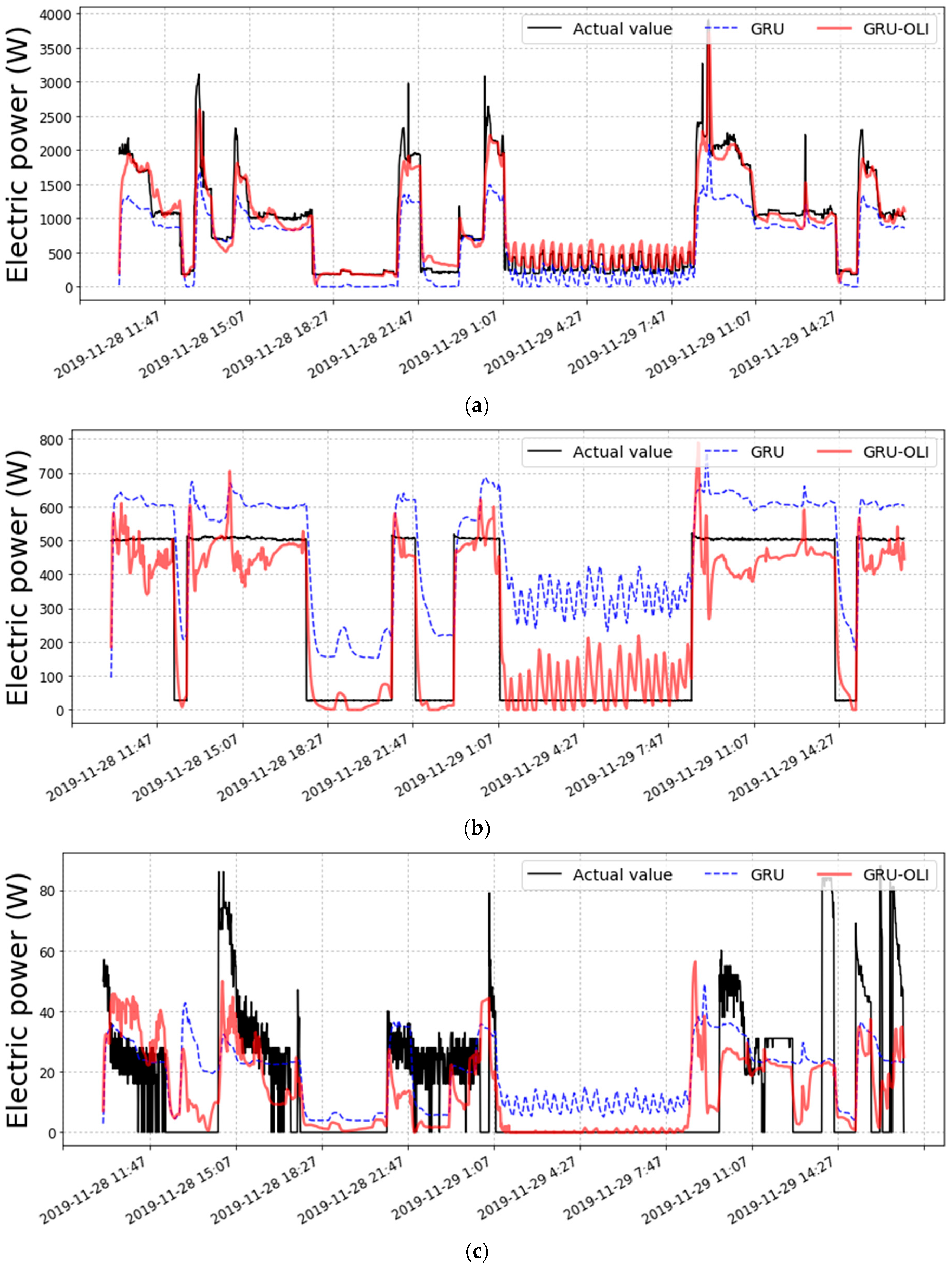
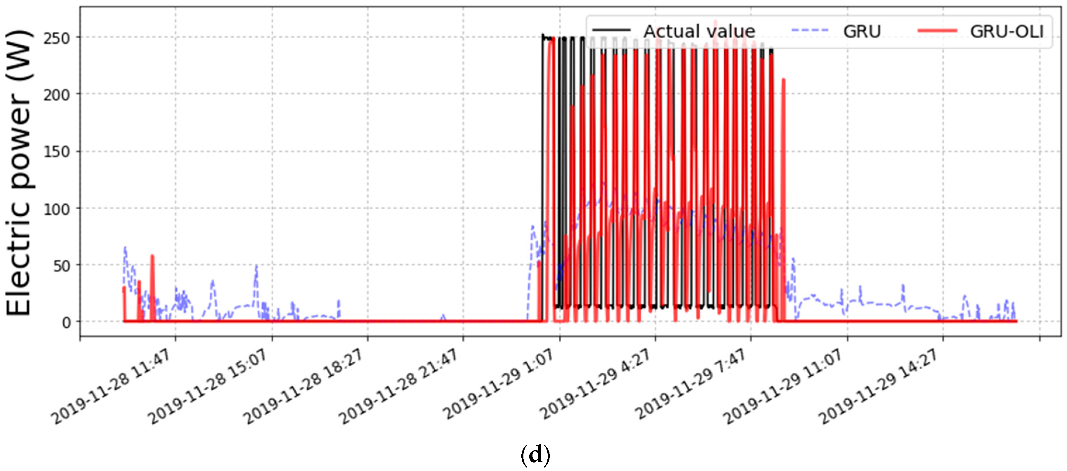
Figure 14 represents the electric power inferring results of the GRU-based disaggregation model using the occupant location information (GRU-OLI) and the GRU-based disaggregation model without the occupant location information. As described in Section 4.5.1, the cases of four representative appliances are shown in the graph. It was confirmed that the overall electric power inferring performance was stabilized when the occupant location information was used. In particular, the results for an air conditioner showed excellent performance, which were very similar to the actual values. In the case of a laptop, when the appliance was not operating, it was inferred more clearly with the occupant’s location information. Additionally, in a case of a hot water mat, electric power was clearly inferred for ON and OFF, and the appliance and the inferring performance of the electric power consumption increased dramatically compared to the one without the occupant location information.

Table 7. Results of the electricity consumption (kWh) disaggregation by appliance including GRU-OLI.

Appliances	Actual Value (kWh)	FHMM (kWh)	LSTM (kWh)	GRU (kWh)	GRU–OLI (kWh)
Air conditioner	27.96	9.90	15.43	19.66	27.47
Lights	9.12	8.16	12.69	14.50	8.87
Desktop	2.52	2.19	2.18	2.59	2.50
ERV	2.03	0.87	2.01	1.81	2.04
Hot water mat	0.81	3.57	0.64	0.92	0.86
Laptop	0.46	0.53	0.51	0.57	0.44
Fridge	0.40	0.71	0.44	0.46	0.39
Washer	0.27	12.72	1.15	0.90	0.31
Air cleaner	0.27	0.16	0.01	0.24	0.25
Rice cooker	0.08	3.79	0.11	0.35	0.32
Microwave	0.07	0.06	0.68	0.24	0.16
Hair dryer	0.04	0.19	0.12	1.16	0.95
TV	0.02	0.36	0.03	0.02	0.02
Humidifier	0	0.32	0.20	0.14	0.08

shows the results of the disaggregation of the electricity consumption by adding the case of the GRU-OLI disaggregation model to Table 4. The GRU-OLI model showed excellent performance in inferring the electricity consumption in 11 out of a total of 14 appliances (appliances other than a rice cooker, microwave range, and hair dryer), which were most similar to the actual values. In the electric power inferring performance results by the minute, as shown in

Table 8. Results of the electric power (W) disaggregation by appliance including GRU-OLI.

Appliances	GRU		GRU–OLI
	MAE	RMSE	MAE	RMSE
Air conditioner	284.35	378.44	131.35	215.35
Lights	178.33	213.26	55.79	74.77
Desktop	12.72	12.92	4.57	5.62
ERV	7.24	7.68	4.20	5.24
Hot water mat	33.70	58.26	15.55	40.13
Laptop	14.46	18.71	10.52	12.59
Fridge	19.78	21.75	17.43	22.23
Washer	31.07	97.25	30.79	92.63
Air cleaner	3.03	4.93	2.39	4.94
Rice cooker	13.08	30.40	12.42	28.13
Microwave	10.12	52.46	7.56	51.09
Hair dryer	38.46	75.77	31.98	61.23
TV	1.27	4.60	1.11	4.30
Humidifier	4.42	5.47	2.85	3.68
Average	46.57	70.14	23.47	44.42

, the inferring performance when using the occupant location information was improved by 50% for the MAE and 37% for the RMSE compared to the model without the location information.

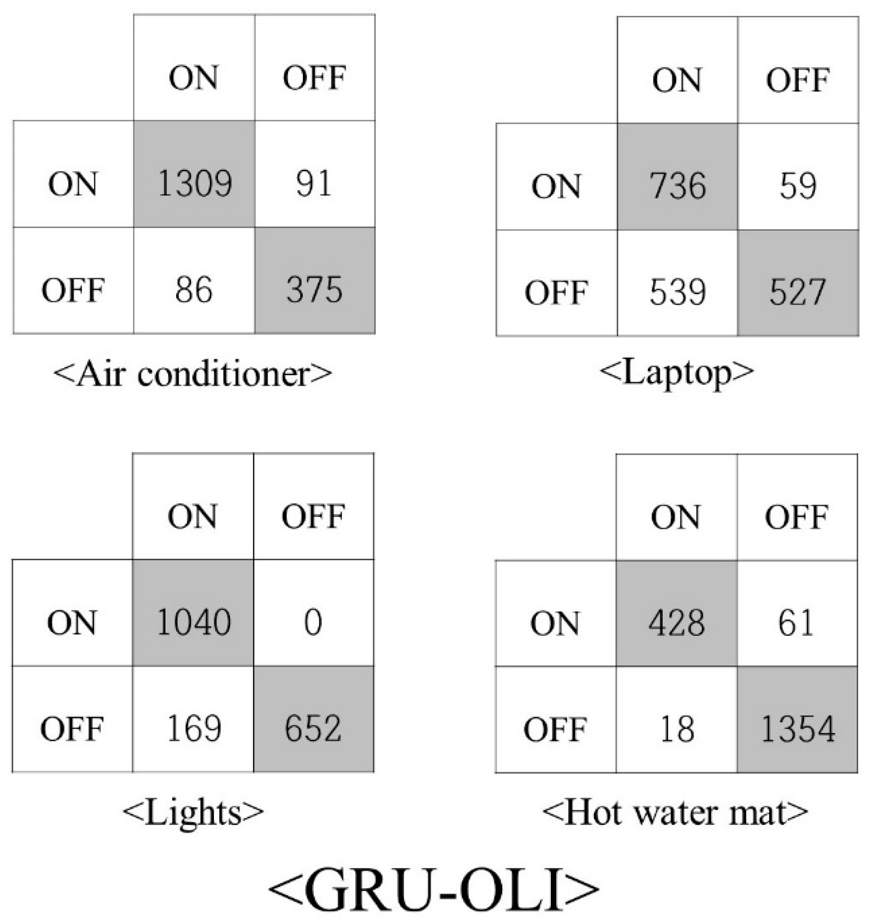
The overall performance of the appliance state estimation was improved, as shown in Figure 15. In particular, the performance of estimating the appliance OFF state improved dramatically in the case of the laptop and the hot water mat by utilizing the occupant location information. As a result of judging based on the average accuracy and F1-score in

Table 9. Performance of the appliance state estimation by algorithm including GRU-OLI.

Appliances	GRU		GRU-OLI
	Accuracy	F1-Score	Accuracy	F1-Score
Air conditioner	0.89	0.85	0.93	0.90
Lights	0.89	0.89	0.91	0.91
Desktop	1.00	1.00	1.00	1.00
ERV	0.99	0.50	1.00	0.50
Hot water mat	0.52	0.52	0.96	0.94
Laptop	0.60	0.59	0.67	0.65
Fridge	0.41	0.41	0.39	0.39
Washer	0.86	0.69	0.89	0.72
Air cleaner	0.34	0.33	0.47	0.43
Rice cooker	0.51	0.36	0.51	0.36
Microwave	0.99	0.50	0.98	0.50
Hair dryer	0.50	0.34	0.50	0.34
TV	0.99	0.50	0.97	0.49
Humidifier	0.54	0.35	0.81	0.45
Average	0.72	0.56	0.79	0.61

, the performance of these appliances improved by 0.07 and 0.05, respectively.

Table 10. The average value of the performance metrics for the FHMM and GRU-OLI.

Value	FHMM				GRU-OLI (Suggested Method)
	MAE	RMSE	Accuracy	F1-Score	MAE	RMSE	Accuracy	F1-Score
Average	103.63	177.08	0.66	0.51	23.47	44.42	0.79	0.61

shows the performance metrics of the existing FHMM model and the model using the GRU-based occupant location information (GRU-OLI). It was confirmed that the performance of NILM based on GRU-OLI showed an improvement by 0.13 in the accuracy, 0.1 in the F1-score, 77% in the MAE, and 75% in the RMSE compared to the existing FHMM. Therefore, it can be said that the occupant location information is a useful input to increase the performance of the NILM.

5. Conclusions

In this study, the performance of the RNN-based algorithm for NILM in a residential environment was investigated and analyzed. The performance of the GRU model with the occupant location information for energy disaggregation was also tested as well. Consequently, when the disaggregation model was formulated with the RNN-based algorithm (GRU algorithm), the performance was improved by 0.06 based on the accuracy, 0.05 based on the F1-score, 55% based on the MAE, and 60% based on the RMSE. In addition, when the occupant location information was used, the performance improved by 0.07 for accuracy, 0.05 for F1-score, 50% for MAE, and 37% for the RMSE compared to the model without the location information. As a result, compared to the existing FHMM-based NILM, the suggested GRU-based model with the occupant location information showed a great improvement in terms of the accuracy, F1-score, MAE, and RMSE. Therefore, a RNN-based algorithm with the occupant location information can contribute to increased performance in the NILM.

This study has great significance in learning and validating an energy disaggregation model with the data collected in a residential environment. It is also meaningful as it shows an advantage of using the occupant location information as nonelectrical information that could increase the performance of energy disaggregation. However, this study had limitations in that data omission may have occurred when converting the data intervals from seconds to minutes in the process of acquiring the occupant location data. Furthermore, the location information could not be obtained if the occupants were covered by the furniture or walls.

Therefore, there are future research plans to explore ways in which to improve the energy disaggregation and localization performance of occupants using data intervals in seconds. In addition, there are also difficulties to obtaining image data in a room including privacy problems for occupants. Thus, our future research includes the development of an occupant behavior detection model without using cameras. The method suggested in this study for energy disaggregation based on a RNN with the occupant location information as an input variable will be of great help in future NILM research such as in detecting abnormal electric power consumption, monitoring the elderly, and increasing the power efficiency.

References

1. Energy Information Administration. International Energy Outlook 2019 (IEO2019); Energy Information Administration: Washington, DC, USA, 2019; Volume 26. [Google Scholar]
2. Korea Energy Economics Institute. Monthly Energy Statistics (2019.04); Korea Energy Economics Institute: Ulsan, Republic of Korea, 2019. [Google Scholar]
3. Kolter, J.Z.; Johnson, M.J. REDD: A Public Data Set for Energy Disaggregation Research. In Proceedings of the Workshop on Data Mining Applications in Sustainability (SIGKDD), San Diego, CA, USA, 21–24 August 2011; No. Citeseer. Volume 25, pp. 59–62. [Google Scholar]
4. Darby, S. The effectiveness of feedback on energy consumption. A Rev. DEFRA Lit. Metering Billing Direct Disp. 2006, 486, 26. [Google Scholar]
5. Ghahramani, Z.; Jordan, M.I. Factorial hidden Markov models. Mach. Learn. 1997, 29, 245–273. [Google Scholar] [CrossRef]
6. Kim, J.; Le, T.T.H.; Kim, H. Nonintrusive load monitoring based on advanced deep learning and novel signature. Comput. Intell. Neurosci. 2017, 2017, 4216281. [Google Scholar] [CrossRef] [PubMed]
7. Bhotto, M.Z.A.; Makonin, S.; Bajić, I.V. Load Disaggregation Based on Aided Linear Integer Programming. IEEE Trans. Circuits Syst. II Express Briefs 2016, 64, 792–796. [Google Scholar] [CrossRef]
8. Balletti, M.; Piccialli, V.; Sudoso, A.M. Mixed-Integer Nonlinear Programming for State-Based Non-Intrusive Load Monitoring. IEEE Trans. Smart Grid 2021, 13, 3301–3314. [Google Scholar] [CrossRef]
9. Gul, M.S.; Patidar, S. Understanding the energy consumption and occupancy of a multi-purpose academic building. Energy Build. 2015, 87, 155–165. [Google Scholar] [CrossRef]
10. Martani, C.; Lee, D.; Robinson, P.; Britter, R.; Ratti, C. ENERNET: Studying the dynamic relationship between building occupancy and energy consumption. Energy Build. 2012, 47, 584–591. [Google Scholar] [CrossRef]
11. Rafsanjani, H.N.; Ahn, C.R.; Chen, J. Linking building energy consumption with occupants’ energy-consuming behaviors in commercial buildings: Non-intrusive occupant load monitoring (NIOLM). Energy Build. 2018, 172, 317–327. [Google Scholar] [CrossRef]
12. Hosseini, S.; Kelouwani, S.; Agbossou, K.; Cardenas, A.; Henao, N. A Semi-Synthetic Dataset Development Tool for Household Energy Consumption Analysis. In Proceedings of the 2017 IEEE International Conference on Industrial Technology (ICIT), Ontario, CA, USA, 22–25 March 2017; pp. 564–569. [Google Scholar]
13. Holmegaard, E.; Kjærgaard, M.B. NILM in an Industrial Setting: A Load Characterization and aAlgorithm Evaluation. In Proceedings of the 2016 IEEE International Conference on Smart Computing (SMARTCOMP), St. Louis, MO, USA, 18–20 May 2016; pp. 1–8. [Google Scholar]
14. Hüsken, M.; Stagge, P. Recurrent neural networks for time series classification. Neurocomputing 2003, 50, 223–235. [Google Scholar] [CrossRef]
15. Akkaya, K.; Guvenc, I.; Aygun, R.; Pala, N.; Kadri, A. IoT-Based Occupancy Monitoring Techniques for Energy-Efficient Smart Buildings. In Proceedings of the 2015 IEEE Wireless Communications and Networking Conference Workshops (WCNCW), New Orleans, LA, USA, 9–12 March 2015; pp. 58–63. [Google Scholar]
16. Diraco, G.; Leone, A.; Siciliano, P. People occupancy detection and profiling with 3D depth sensors for building energy management. Energy Build. 2015, 92, 246–266. [Google Scholar] [CrossRef]
17. Uotila, V.; Skogster, P. Space management in a DIY store analyzing consumer shopping paths with data-tracking devices. Facilities 2007, 25, 363–374. [Google Scholar] [CrossRef]
18. Paolini, G.; Del Prete, M.; Berra, F.; Masotti, D.; Costanzo, A. An Agile and Accurate Microwave System for Tracking Elderly People Occupancy at Home. In Proceedings of the 2016 IEEE MTT-S Latin America Microwave Conference (LAMC), Puerto Vallarta, Mexico, 12–14 December 2016; pp. 1–3. [Google Scholar]
19. Mirshekari, M.; Pan, S.; Fagert, J.; Schooler, E.M.; Zhang, P.; Noh, H.Y. Occupant localization using footstep-induced structural vibration. Mech. Syst. Signal Process. 2018, 112, 77–97. [Google Scholar] [CrossRef]
20. Henry, P.; Krainin, M.; Herbst, E.; Ren, X.; Fox, D. RGB-D mapping: Using Kinect-style depth cameras for dense 3D modeling of indoor environments. Int. J. Robot. Res. 2012, 31, 647–663. [Google Scholar] [CrossRef]
21. Liu, S.; Yin, L.; Ho, W.K.; Ling, K.V.; Schiavon, S. A tracking cooling fan using geofence and camera-based indoor localization. Build. Environ. 2017, 114, 36–44. [Google Scholar] [CrossRef]
22. Drira, S.; Reuland, Y.; Pai, S.G.; Noh, H.Y.; Smith, I.F. Model-based occupant tracking using slab-vibration measurements. Front. Built Environ. 2019, 5, 63. [Google Scholar] [CrossRef]
23. Moussa, M.; Youssef, M. Smart Devices for Smart Environments: Device-Free Passive Detection in Real Environments. In Proceedings of the 2009 IEEE International Conference on Pervasive Computing and Communications, Galveston, TX, USA, 9–13 March 2009; pp. 1–6. [Google Scholar]
24. Youssef, M.; Mah, M.; Agrawala, A. Challenges: Device-Free Passive Localization for Wireless Environments. In Proceedings of the 13th Annual ACM International Conference on Mobile Computing and Networking, Montreal, QC, Canada, 9–14 September 2007; pp. 222–229. [Google Scholar]
25. Zhen, Z.N.; Jia, Q.S.; Song, C.; Guan, X. An indoor localization algorithm for lighting control using RFID. In Proceedings of the 2008 IEEE Energy 2030 Conference, Atlanta, GA, USA, 17–18 November 2008; pp. 1–6. [Google Scholar]
26. Chintalapudi, K.; Padmanabha Iyer, A.; Padmanabhan, V.N. Indoor Localization without the Pain. In Proceedings of the 16th Annual International Conference on Mobile Computing and Networking, Chicago, IL, USA, 20–24 September 2010; pp. 173–184. [Google Scholar]
27. Anderson, K.D.; Bergés, M.E.; Ocneanu, A.; Benitez, D.; Moura, J.M. Event Detection for Non-intrusive Load Monitoring. In Proceedings of the IECON 2012-38th Annual Conference on IEEE Industrial Electronics Society, Montreal, CA, USA, 25–28 October 2012; pp. 3312–3317. [Google Scholar]
28. Zeifman, M.; Roth, K. Nonintrusive appliance load monitoring: Review and outlook. IEEE Trans. Consum. Electron. 2011, 57, 76–84. [Google Scholar] [CrossRef]
29. Hart, G.W. Nonintrusive appliance load monitoring. Proc. IEEE 1992, 80, 1870–1891. [Google Scholar] [CrossRef]
30. Powers, J.T.; Margossian, B.; Smith, B.A. Using a rule-based algorithm to disaggregate end-use load profiles from premise-level data. IEEE Comput. Appl. Power 1991, 4, 42–47. [Google Scholar] [CrossRef]
31. Laughman, C.; Lee, K.; Cox, R.; Shaw, S.; Leeb, S.; Norford, L.; Armstrong, P. Power signature analysis. IEEE Power Energy Mag. 2003, 1, 56–63. [Google Scholar] [CrossRef]
32. Akbar, M.; Khan, Z.A. Modified Nonintrusive Appliance Load Monitoring for Nonlinear Devices. In Proceedings of the 2007 IEEE International Multitopic Conference, Lahore, Pakistan, 28–30 December 2007; pp. 1–5. [Google Scholar]
33. Batra, N.; Wang, H.; Singh, A.; Whitehouse, K. Matrix Factorization for Scalable Energy Breakdown. In Proceedings of the AAAI Conference on Artificial Intelligence, New York, NY, USA, 4–9 February 2017. [Google Scholar]
34. Yue, H.; Yan, K.; Zhao, J.; Ren, Y.; Yan, X.; Zhao, H. Estimating Demand Response Flexibility of Smart Home Appliances via NILM Algorithm. In Proceedings of the 2020 IEEE 4th Information Technology, Networking, Electronic and Automation Control Conference (ITNEC), Chongqing, China, 1 June 2020; pp. 394–398. [Google Scholar]
35. Zoha, A.; Gluhak, A.; Imran, M.A.; Rajasegarar, S. Non-intrusive load monitoring approaches for disaggregated energy sensing: A survey. Sensors 2012, 12, 16838–16866. [Google Scholar] [CrossRef]
36. Abubakar, I.; Khalid, S.N.; Mustafa, M.W.; Shareef, H.; Mustapha, M. Application of load monitoring in appliances’ energy management—A review. Renew. Sustain. Energy Rev. 2017, 67, 235–245. [Google Scholar] [CrossRef]
37. Cypriano, J.G.; Juca, J.L.; da Silva, L.C.; Azzini, H.A. Load Disaggregation Development Project: A NILM Proposal for Energy Usage Changes. In Proceedings of the Applied Energy Symposium, MIT A+B, Boston, MA, USA, 22–24 May 2019; Available online: https://www.energy-proceedings.org/wp-content/uploads/2020/01/AEAB2019_paper_241.pdf (accessed on 1 May 2022).
38. Kim, H.; Marwah, M.; Arlitt, M.; Lyon, G.; Han, J.; Society for Industrial and Applied Mathematics. Unsupervised Disaggregation of Low-Frequency Power Measurements. In Proceedings of the 2011 SIAM International Conference on Data Mining, Mesa, AZ, USA, 28–30 April 2011; pp. 747–758. [Google Scholar]
39. Zeifman, M.; Roth, K. Disaggregation of Home Energy Display Data Using a Probabilistic Approach. In Proceedings of the 2012 IEEE International Conference on Consumer Electronics (ICCE), Las Vegas, NV, USA, 13–16 January 2012; pp. 630–631. [Google Scholar]
40. Joo, I.T.; Choi, S.H. Stock Prediction Model based on Bidirectional LSTM Recurrent Neural Network. J. Korea Inst. Inf. Electron. Commun. Technol. 2018, 11, 204–208. [Google Scholar]
41. Hochreiter, S. The vanishing gradient problem during learning recurrent neural nets and problem solutions. Int. J. Uncertain. Fuzziness Knowl.-Based Syst. 1998, 6, 107–116. [Google Scholar] [CrossRef]
42. Hochreiter, S.; Schmidhuber, J. Long short-term memory. Neural Comput. 1997, 9, 1735–1780. [Google Scholar] [CrossRef] [PubMed]
43. Cho, K.; Van Merriënboer, B.; Gulcehre, C.; Bahdanau, D.; Bougares, F.; Schwenk, H.; Bengio, Y. Learning phrase representations using RNN encoder-decoder for statistical machine translation. arXiv 2014, arXiv:1406.1078. [Google Scholar]
44. Valueva, M.V.; Nagornov, N.N.; Lyakhov, P.A.; Valuev, G.V.; Chervyakov, N.I. Application of the residue number system to reduce hardware costs of the convolutional neural network implementation. Math. Comput. Simul. 2020, 177, 232–243. [Google Scholar] [CrossRef]
45. Eom, Y.H.; Yoo, J.W.; Hong, S.B.; Kim, M.S. Refrigerant charge fault detection method of air source heat pump system using convolutional neural network for energy saving. Energy 2019, 187, 115877. [Google Scholar] [CrossRef]
46. Redmon, J.; Farhadi, A. Yolov3: An incremental improvement. arXiv 2018, arXiv:1804.02767. [Google Scholar]
47. Willmott, C.J.; Matsuura, K. Advantages of the mean absolute error (MAE) over the root mean square error (RMSE) in assessing average model performance. Clim. Res. 2005, 30, 79–82. [Google Scholar] [CrossRef]
48. Chai, T.; Draxler, R.R. Root mean square error (RMSE) or mean absolute error (MAE)?–Arguments against avoiding RMSE in the literature. Geosci. Model Dev. 2014, 7, 1247–1250. [Google Scholar] [CrossRef]
49. Willmott, C.J. Some comments on the evaluation of model performance. Bull. Am. Meteorol. Soc. 1982, 63, 1309–1313. [Google Scholar] [CrossRef]
50. Batra, N.; Kelly, J.; Parson, O.; Dutta, H.; Knottenbelt, W.; Rogers, A.; Singh, A.; Srivastava, M. NILMTK: An Open Source Toolkit for Non-intrusive Load Monitoring. In Proceedings of the 5th International Conference on Future Energy Systems, Cambridge, UK, 11–13 June 2014; pp. 265–276. [Google Scholar]
51. Kohavi, R. A Study of Cross-Validation and Bootstrap for Accuracy Estimation and Model Selection. In Proceedings of the International Joint Conference on Artificial Intelligence, Montreal, QC, Canada, 20–25 August 1995; pp. 1137–1145. [Google Scholar]
52. Hsu, C.W.; Chang, C.C.; Lin, C.J. A Practical Guide to Support Vector Classification; Tech. Rep.; Department of Computer Science, National Taiwan University: Taipei City, Taiwan, 2003. [Google Scholar]
Figure 1. Concept of nonintrusive load monitoring (NILM).
Energies 16 03688 g001
Figure 2. Structure of factorial hidden Markov model.
Energies 16 03688 g002
Figure 3. Pictures of the Smart Living Testbed: (a) perspective view; (b) outside view; (c) living room; (d) bedroom.
Energies 16 03688 g003
Figure 4. Example of electric power data by 14 appliances from the SLT.
Energies 16 03688 g004
Figure 5. Structure of recurrent neural networks.
Energies 16 03688 g005
Figure 6. Structure of a long short-term memory.
Energies 16 03688 g006
Figure 7. Structure of gated recurrent units.
Energies 16 03688 g007
Figure 8. Structure of convolution neural networks.
Energies 16 03688 g008
Figure 9. Example of the YOLOv3-based occupant detection and pointing.
Energies 16 03688 g009
Figure 10. Process of a perspective transformation: (a) specifying a vertex; (b) the OpenCV-based perspective transformation.
Energies 16 03688 g010
Figure 11. Generating the occupant location coordinates.
Energies 16 03688 g011
Figure 12. Example of power (W) disaggregation result based on the FHMM and RNN (LSTM and GRU): (a) air conditioner; (b) lighting; (c) laptop; (d) hot water mat.
Energies 16 03688 g012aEnergies 16 03688 g012b
Figure 13. Confusion matrix (four representative appliances) estimating the appliance states: (a) FHMM; (b) LSTM; (c) in GRU.
Energies 16 03688 g013
Figure 14. Example of the power (W) disaggregation results in GRU with and without the occupant location information (OLI): (a) air conditioner; (b) lights; (c) laptop; (d) hot water mat.
Energies 16 03688 g014aEnergies 16 03688 g014b
Figure 15. Confusion matrix (four appliances) estimating the appliance states in GRU-OLI.
Energies 16 03688 g015