Multi-Horizon Wind Power Forecasting Using Multi-Modal Spatio-Temporal Neural Networks

Abstract

Wind energy represents one of the leading renewable energy sectors and is considered instrumental in the ongoing decarbonization process. Accurate forecasts are essential for a reliable large-scale wind power integration, allowing efficient operation and maintenance, planning of unit commitment, and scheduling by system operators. However, due to non-stationarity, randomness, and intermittency, forecasting wind power is challenging. This work investigates a multi-modal approach for wind power forecasting by considering turbine-level time series collected from SCADA systems and high-resolution Numerical Weather Prediction maps. A neural architecture based on stacked Recurrent Neural Networks is proposed to process and combine different data sources containing spatio-temporal patterns. This architecture allows combining the local information from the turbine’s internal operating conditions with future meteorological data from the surrounding area. Specifically, this work focuses on multi-horizon turbine-level hourly forecasts for an entire wind farm with a lead time of 90 h. This work explores the impact of meteorological variables on different spatial scales, from full grids to cardinal point features, on wind power forecasts. Results show that a subset of features associated with all wind directions, even when spatially distant, can produce more accurate forecasts with respect to full grids and reduce computation times. The proposed model outperforms the linear regression baseline and the XGBoost regressor achieving an average skill score of 25%. Finally, the integration of SCADA data in the training process improved the predictions allowing the multi-modal neural network to model not only the meteorological patterns but also the turbine’s internal behavior.

1. Introduction

Wind energy is promoted worldwide as a core energy source for the mitigation of climate change, allowing for the reduction of carbon emissions while having declining capital costs driven by wind turbine technological advancements [1,2]. However, the rapid increase in wind power energy production on a global scale has created new challenges with respect to grid integration, due to the non-stationarity, randomness, and intermittency of wind [3]. Accurate real-time forecasting algorithms can help to mitigate these problems and reduce the cost impacts of wind to a large extent by making wind power more schedulable. Hence, forecasting models have a significant economic and technical impact on the system by increasing wind power penetration and allowing efficient operation and maintenance, planning of unit commitment, and scheduling by system operators [4].

Wind power forecasting methods can generally be grouped into physical, data-driven, and hybrid methods, and a detailed classification is provided by Yousuf et al. [5]. This work focuses on data-driven methods, specifically approaches based on Machine Learning (ML), which have proven their ability to capture non-linear wind patterns in many recent works (see the paper by Jørgensen et al. [6] for an overview). In particular, it is of interest to explore how the combination of different data sources, i.e., multi-modal data, can impact and improve predictions of data-driven algorithms. Since it is rare that a single modality provides complete knowledge of the phenomenon of interest, performing data fusion starting from multiple modalities can provide insights and benefits to forecasting models by contributing to a more unified picture and global view of the system [7].

Multi-modal approaches have recently been employed across a wide variety of applications concerning climate and energy forecasting. Boussioux et al. [8] introduce an ML framework for tropical cyclone intensity and track forecasting, and show that, when combining historical storm data, reanalysis maps and historical operational forecasts, prediction errors comparable to current operational forecast models can be achieved while computing in seconds. Yang et al. [9] propose a multi-modal deep learning method for forecasting the daily power generation of small hydropower stations. In this work, the authors combine daily power generation and precipitation data, together with the spatial distribution of precipitation observed by meteorological satellite remote sensing, and conclude that a multi-modal neural network can effectively improve the accuracy of forecasts. The work of Haputhanthri et al. [10] employs two Long Short-Term Memory (LSTM) networks that process a stream of sky images, time series of past solar irradiance readings, and cloud cover readings as inputs for irradiance nowcasting. Du et al. [11] present an ensemble ML-based method to forecast wind power production, which uses both the wind generation forecasted by a Numerical Weather Prediction (NWP) model and the meteorological observation data from weather stations. The experimental results show that the proposed ensemble method based on Artificial Neural Networks (ANN), support vector regressions, and Gaussian processes can improve the performance of 3-h ahead wind forecasting with respect to NWP forecasts.

The present work casts the task of wind power forecasting in a multi-modal framework by considering the NWP data provided by the European Centre for Medium-Range Weather Forecasts (ECMWF) and the data collected from the Supervisory Control Furthermore, Data Acquisition (SCADA) systems of the “La Haute Borne” wind farm, made available by Engie [12] and one of the few datasets with an open license, as reported by Effenberger et al. [13]. Other papers have combined NWP and SCADA data but never considered NWP on a mesoscale level as input to the model together with turbine operational measurements. For example, Donadio et al. [14] proposed an ANN that takes in input meteorological variables (temperature, pressure, wind speed, and direction) interpolated at the wind turbine locations and uses SCADA signals as turbine-level power outputs rather than predictors for the model. Another example is the work of Zheng et al. [15], where the authors use meteorological predictions obtained in the vicinity of the wind farm installation site to predict wind speed and, then, train a second model to map wind predictions to power outputs. Furthermore, in this case, the SCADA data are employed only as ground truth for the model.

This paper, instead, considers High-RESolution (HRES) NWP forecasts in the form of incrementally larger maps and SCADA time series as input for the predictive model to investigate how the area surrounding a wind farm and the turbine’s internal operating conditions can impact the forecasts of the power output. NWP maps are in the form of regular square grids on a mesoscale level centered around the wind farm, and the choice of including a larger area and not only the meteorological data closest to the specific farm location was motivated by the presence of patterns that evolve both in time and space. It is important to note that NWP systems are better at predicting on a large scale than with precision at specific locations. Therefore, it is not uncommon for an NWP forecast to be in error when it comes to the precise position and fine-scale structure of weather features, as reported by Cutler et al. [16]. Therefore, meteorological variables on different spatial scales, from full grids to cardinal point features, are downscaled to the farm location and mapped to turbine-level power outputs by training a data-driven model able to capture wind patterns over larger areas. In this way, the model learns the downscaling transfer function and the power curves of the turbines altogether.

In detail, this paper proposes a spatio-temporal neural network for wind power forecasting with a lead time of up to 90 h. The model is composed of two sub-networks based on stacked Recurrent Neural Networks (RNNs) with LSTM cells that process, respectively, the SCADA and the HRES data. The outputs of the two modules are combined using a non-linear gating mechanism that regulates the flow of HRES information used for wind power forecasting based on the turbine behavior.

The model is tested on four wind turbines with a rated power of 2050 kW, part of the “La Haute Borne” wind farm, for a period that spans four years of operation.

The rest of the paper is organized as follows. Section 2 describes the different data sources and Section 4 presents the architecture of the proposed spatio-temporal neural network, together with the performance metrics used to evaluate the model. Finally, Section 6 presents and discusses the wind power forecasting results, and Section 7 summarizes the present work and draws some conclusions.

2. Multi-Modal Data

As we aim to build a forecasting model that uses several data sources, this section introduces the multi-modal data considered to train and validate the model. Namely, the first source consists of turbine-level time series collected from SCADA systems, and information is provided about the wind farm size, location, and layout, together with turbine-specific details and the monitored variables. The second source consists of high-resolution NWP maps and information is provided about their size, resolution, centering position, and the variables considered for the analysis.

2.1. SCADA Data

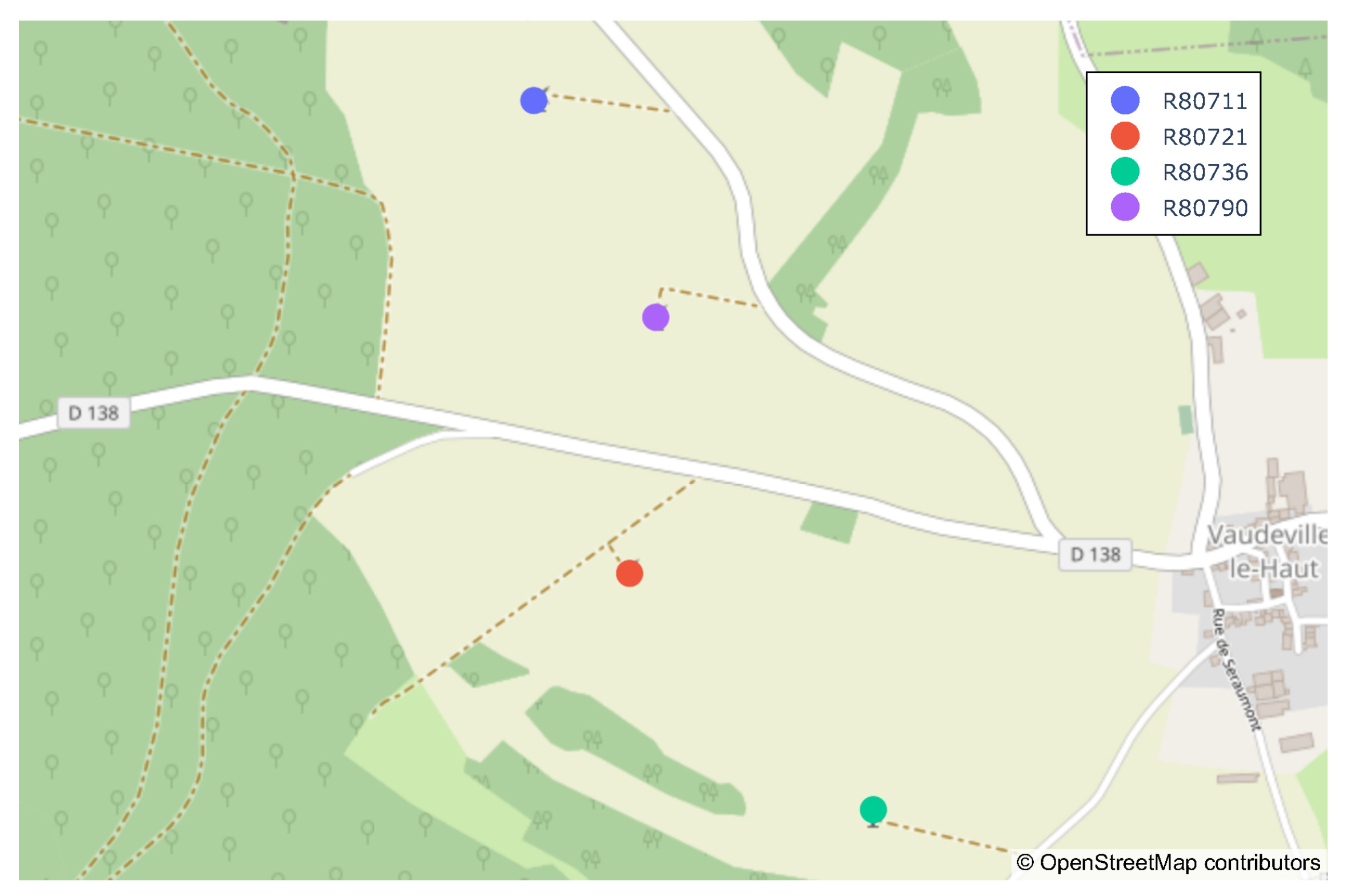
The SCADA data considered are the open data of the "La Haute Borne" wind farm made available by Engie [12], located in the Meuse department of northeastern France. The wind farm is composed of four identical MM82 wind turbines produced by Senvion (identified as R80711, R80721, R80736, and R80790 in Figure 1), each having a rated power of 2050 kW. All turbines have a hub height of 80 m, a rotor diameter of 82 m, and an altitude of 411 m. The dataset includes SCADA signals collected from all four wind turbines sampled every 10 min. In addition to active power, other variables are monitored, such as wind speed, ambient temperature, or gearbox temperature.

This study considers 4 years of operation, ranging from January 2014 to December 2017. In particular, the first two years are selected as training set, the third as validation set, and the last as test set (2:1:1 ratio). In this way, each set contains a complete seasonal cycle.

2.2. NWP Data

The NWP data explored in this work are provided by the European Centre for Medium-Range Weather Forecasts (ECMWF). Specifically, this work considers the highest-resolution atmospheric model providing 10-day forecasts [17], which uses observations and prior information about the Earth system in the form of physical and dynamic representations of the atmosphere. This model produces 4 forecast runs per day (midnight, 6 am, noon, and 6 pm) with hourly steps to step 90 for all four runs, 3-hourly steps from step 93 to 144 and 6-hourly steps from step 150 to 240 for the midnight and noon runs. Forecasts are available on a regular grid for different variables such as temperature, total precipitation, and wind speed.

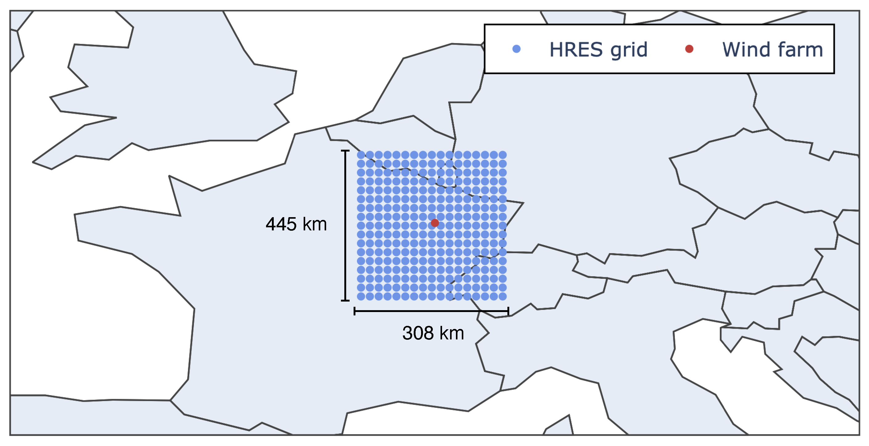
In this paper, midnight runs are considered on a $0.{25}^{\circ }\times 0.{25}^{\circ }$ resolution grid up to step 90, thus having hourly high-resolution forecasts. In particular, a $17\times 17$ map centered around the “La Haute Borne” wind farm (approximately a 308 km × 445 km patch as shown in Figure 2) is considered with the variables horizontal speed of air moving towards the east (U wind speed component) and the north (V wind speed component), at a height of 100 m above the surface of the Earth, together with wind gusts at 10 m height, at each grid point.

3. Data Processing

Both data sources are preprocessed and augmented before the training of the proposed spatio-temporal neural network.

The SCADA sensor signals are standardized, namely by removing the mean and scaling to unit variance. Outlier removal is then carried out using the 6-sigma rule to filter out only extreme outliers caused by sensor measurement errors [18]. Since the proposed model integrates turbine-level knowledge into the forecasts, it is also of interest to include anomalous samples and conditions in the training set to capture possible machine inefficiencies and failures. Finally, SCADA signals are linearly interpolated to deal with missing values and resampled hourly to match the NWP prediction step.

Normalization is applied to the HRES variables, considering samples from the whole grid at all prediction steps. Since weather data have a clear daily periodicity, two extra synthetic signals are generated as input for the neural network. In particular, they are sine and cosine transformations of time and read as

$$f_{sin}\left(s\right)=sin(s·\frac{2\pi }{86400}),$$

$$f_{cos}\left(s\right)=cos(s·\frac{2\pi }{86400}),$$

where s represents time measured in seconds and 86,400 is the total number of seconds in a day. These two synthetic signals are added as extra features to each HRES grid point.

Since the dataset presents only a few short periods of turbine shutdowns compared to normal operating conditions, the training set is augmented to allow the model to capture these scenarios. In fact, for each training year, data are duplicated and the active power is set to zero. The monitored wind speed is left unaltered, enforcing a condition in which turbines do not produce power even though the wind speed falls between the cut-in and cut-off range. The spatio-temporal neural network is then trained on both the original and the augmented versions of the data.

4. Spatio-Temporal Neural Network

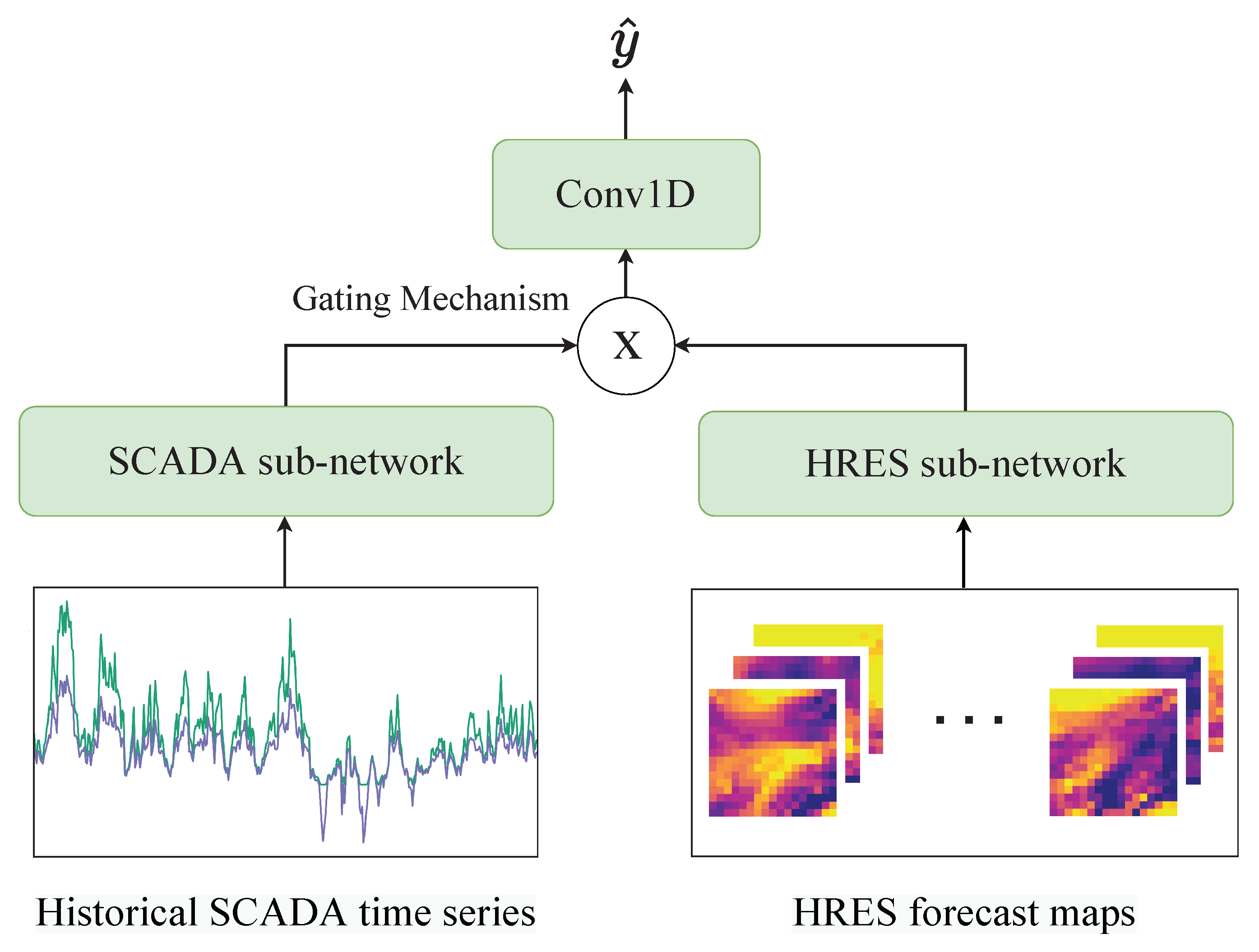
The proposed multi-modal neural network processes and combines the two different data sources previously discussed to produce wind power forecasts. The first includes variables monitored by the SCADA system in the form of time series and provides the model information about the internal behavior and performance of the wind turbines. The second source includes HRES forecasts in the form of regular square maps centered around the wind farm of interest, one for each lead time. In this way, the network can access the meteorological forecasts associated not only with the location of the wind farm but also with the surrounding area, thus capturing patterns that evolve both in time and space.

The network is composed of two sub-networks, referred to as SCADA sub-network and HRES sub-network, that process, respectively, the two data sources, and combine them using a gating mechanism, as shown in Figure 3. The building block of each sub-network is a RNN with a LSTM cell [19].

The network is trained using the Backpropagation algorithm considering the $L_1$ loss function, the Adam optimizer, and early stopping to avoid overfitting. Next, the neural architecture is described in detail.

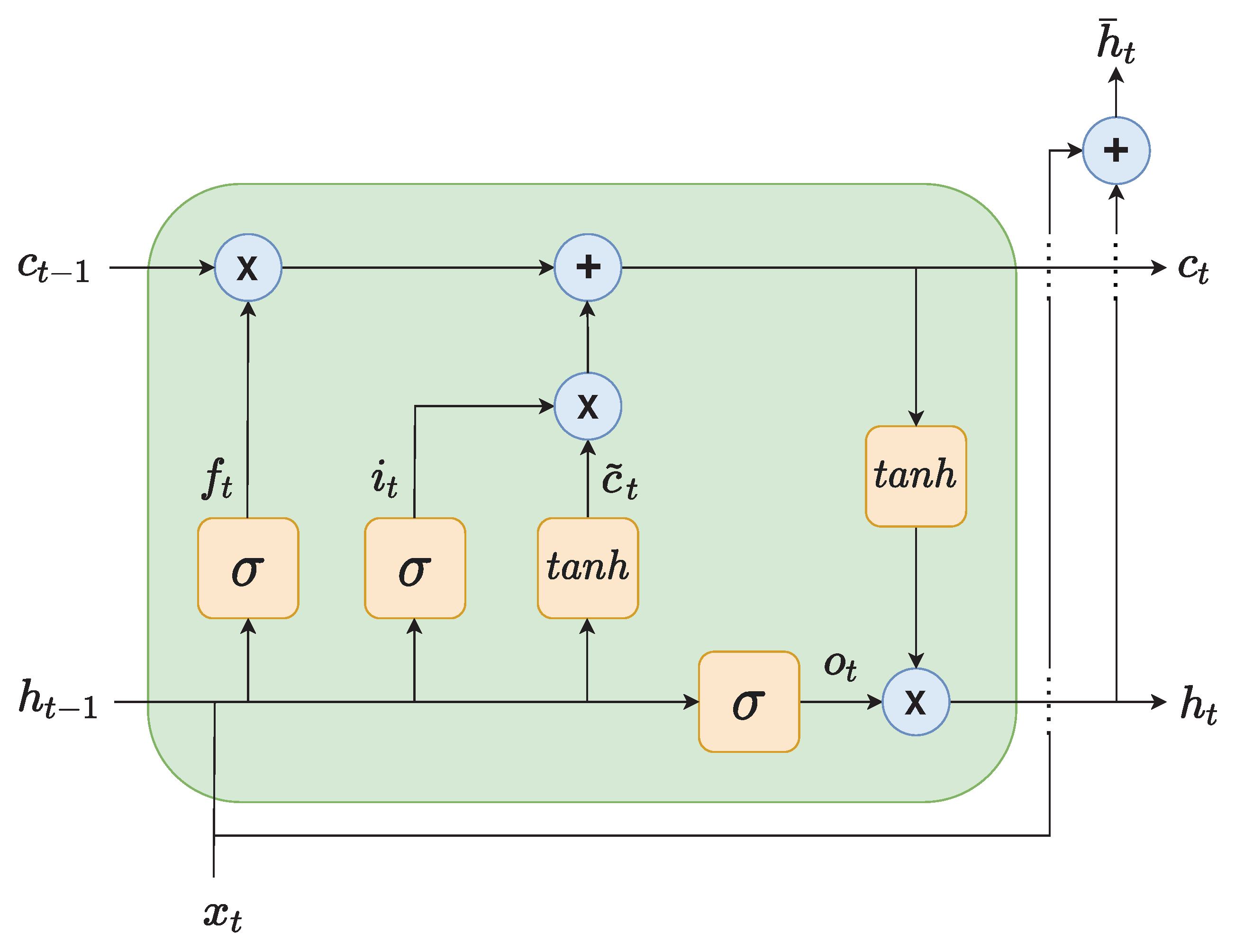
4.1. LSTM

LSTMs use a memory cell and a gating mechanism that contains three non-linear gates, namely, an input gate $i_t$, an output gate $o_t$ and a forget gate $f_t$. These gates allow regulating the flow of information into and out of the cell, to capture both short and long-term dependencies. LSTM cells are formulated as follows

$$f_t=\sigma (W_f·x_t+U_f·h_{t-1}+b_f)$$

$$i_t=\sigma (W_i·x_t+U_i·h_{t-1}+b_i)$$

$$o_t=\sigma (W_o·x_t+U_o·h_{t-1}+b_o)$$

$${\tilde{c}}_t=tanh(W_c·x_t+U_c·h_{t-1}+b_c)$$

$$c_t=f_t\circ c_{t-1}+i_t\circ {\tilde{c}}_t$$

$$h_t=o_t\circ tanh\left(c_t\right),$$

where $x_t$, $h_t$ and $c_t$ are the input, hidden state vector and cell state vector at time step t, respectively, $\sigma$ and $tanh$ are the sigmoid and hyperbolic activation functions, and ∘ denotes the Hadamard product. $W_f$, $U_f$, $b_f$, $W_i$, $U_i$, $b_i$, $W_o$, $U_o$, $b_o$, $W_c$, $U_c$, $b_c$ represent the trainable weights of the network. Moreover, residual connections are added as follows

$${\overline{h}}_t=x_t+h_t,$$

(1)

where ${\overline{h}}_t$ represents the output of the LSTM cell at time step t, as shown also in Figure 4. In this way, gradients can flow through the network directly, without passing through non-linear activation functions, thus preventing gradients to explode or vanish. It is possible to stack multiple LSTM layers by feeding the output ${\overline{h}}_t$ of the previous layer as input $x_t$ for the next.

4.2. SCADA Sub-Network

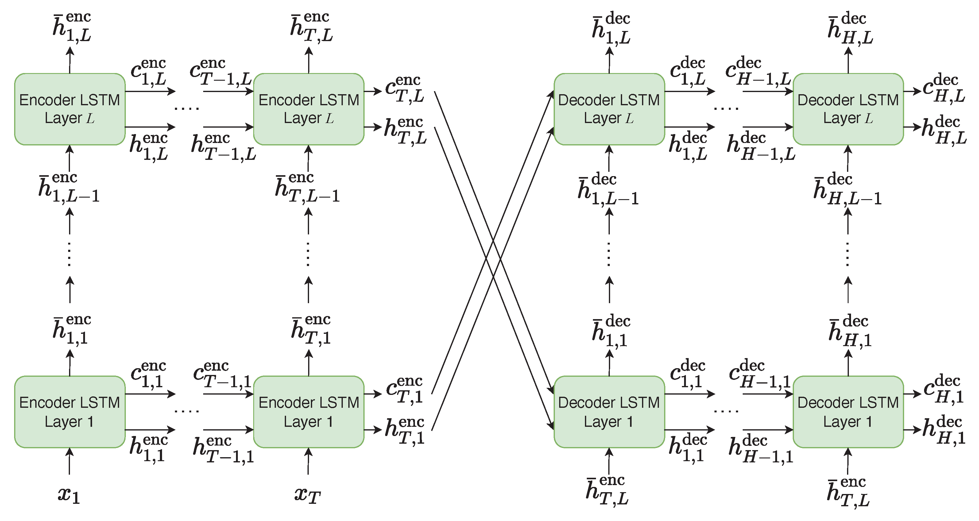
The SCADA sub-network is composed of an encoder and a decoder, as shown in Figure 5. The encoder takes $x=(x_1,\dots ,x_t,\dots ,x_T)$ as input, where $x_t$ represents a multivariate sample of SCADA measurements at time step t, being T the length of the input window. The encoder has L stacked LSTM layers and produces ${\overline{h}}^{\mathrm{enc}}=({\overline{h}}_{1,L}^{\mathrm{enc}},\dots ,{\overline{h}}_{t,L}^{\mathrm{enc}},\dots ,{\overline{h}}_{T,L}^{\mathrm{enc}})$ as output, together with a hidden state vector $h_{T,l}^{\mathrm{enc}}$ and a cell state vector $c_{T,l}^{\mathrm{enc}}$ for each layer l. The decoder has a symmetrical formulation with respect to the decoder. In fact, it is composed of L layers and the LSTM cell of layer l is initialized using the hidden state vector and the cell state vector produced by the encoder at layer $L-l$. The decoder takes $x^{\mathrm{dec}}=({\overline{h}}_{T,L}^{\mathrm{enc}},\dots ,{\overline{h}}_{T,L}^{\mathrm{enc}},\dots ,{\overline{h}}_{T,L}^{\mathrm{enc}})$ as input, namely the output of the last encoder layer L at the last time step T repeated for each time step t, where t goes from 1 to the forecast horizon H. The decoder produces ${\overline{h}}^{\mathrm{SCADA}}=({\overline{h}}_{1,L}^{\mathrm{dec}},\dots ,{\overline{h}}_{t,L}^{\mathrm{dec}},\dots ,{\overline{h}}_{H,L}^{\mathrm{dec}})$ as output, where ${\overline{h}}_{t,L}^{\mathrm{dec}}$ is the output vector computed for time step t.

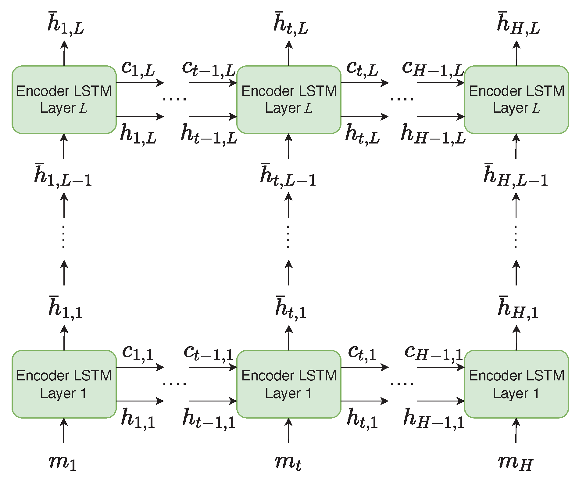
4.3. HRES Sub-Network

The HRES sub-network has no decoder component since the input sequence length matches the output length H as shown in Figure 6. It takes in input $m=(m_1,\dots ,m_t,\dots ,m_T)$, where $m_t$ represents a HRES multivariate forecast map or a spatial sub-section of it at time step $t=1,\dots ,H$. The network has L stacked LSTM layers and produces ${\overline{h}}^{\mathrm{HRES}}=({\overline{h}}_{1,L},\dots ,{\overline{h}}_{t,L},\dots ,{\overline{h}}_{H,L})$ as output, where ${\overline{h}}_{t,L}$ is the output vector computed for time step t.

Both sub-networks are bidirectional to allow the model to retain information from past (backward) and future (forward) time steps. In fact, the outputs of two separate networks, one processing the original input sequences and one the input sequences in reversed order, are concatenated.

4.4. Gating Mechanism

If the output tensors ${\overline{h}}^{\mathrm{SCADA}}$ and ${\overline{h}}^{\mathrm{HRES}}$ have the same dimension, they can be combined as

$$\overline{h}=\sigma ({\overline{h}}^{\mathrm{SCADA}})\circ {\overline{h}}^{\mathrm{HRES}},$$

where $\sigma$ is the sigmoid activation function and ∘ denotes the Hadamard product. In this way, the SCADA hidden vector acts as a non-linear gate, allowing to regulate the flow of HRES information considered for wind power forecasting based on the turbine operating conditions. This gating mechanism is possible when the two sub-networks have the same number of neurons in the last layer.

4.5. Output Layer

Finally, $\overline{h}$ passes through a 1D Convolutional layer and is mapped to the output dimension. Wind power forecasts are produced for each lead time up to step H, making the proposed neural network effectively a multi-horizon model.

5. Spatial Features Analysis

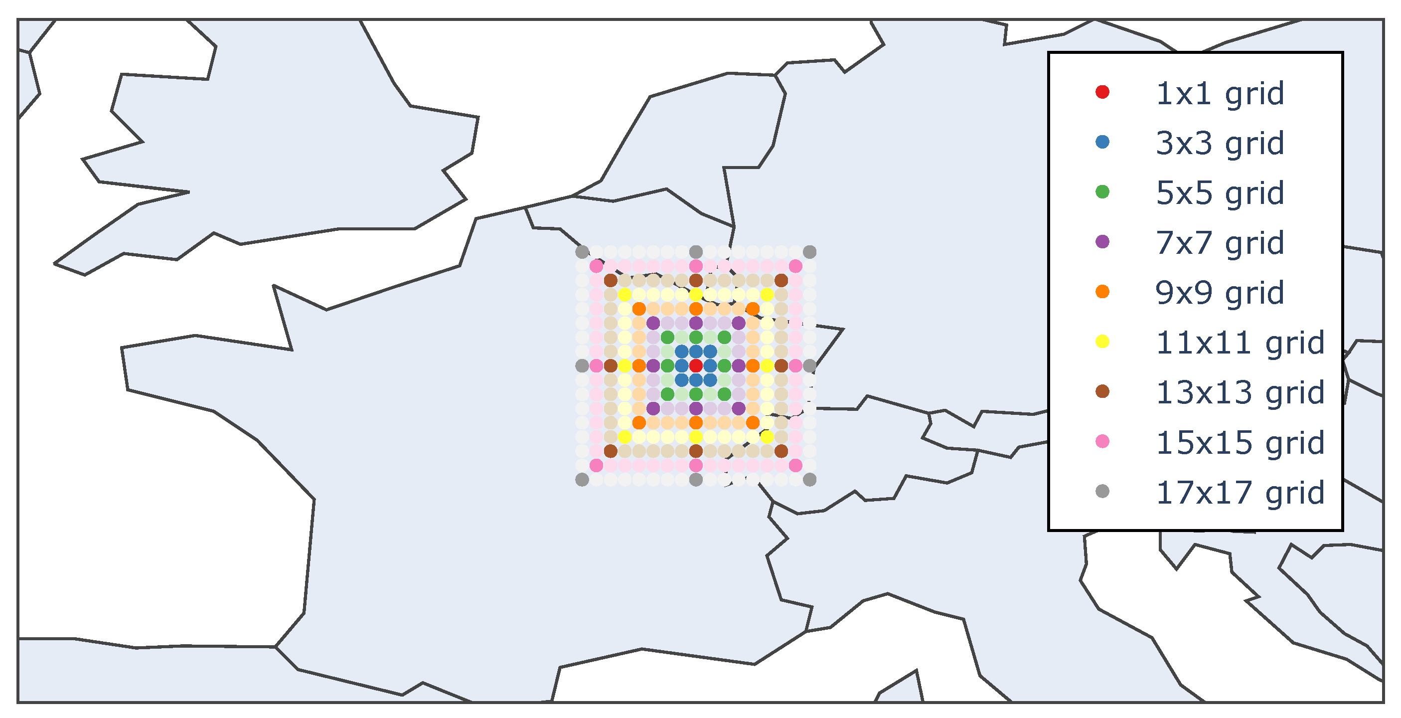
To explore the spatial input features, different incremental map sizes are considered in the form of regular grids and then for each map size, a subset of features is selected to train different models, thereby reducing the input’s dimensionality and improving the learner’s performance.

Considering different map sizes helps to evaluate and understand how the area surrounding the wind farm impacts wind power forecasting, and nine separate models can be trained using incrementally larger HRES forecast maps, with sizes ranging from $1\times 1$ to $17\times 17$. Figure 7 shows an example of a map of size $9\times 9$, where thus a square grid of 81 points is provided as spatial features to the neural network.

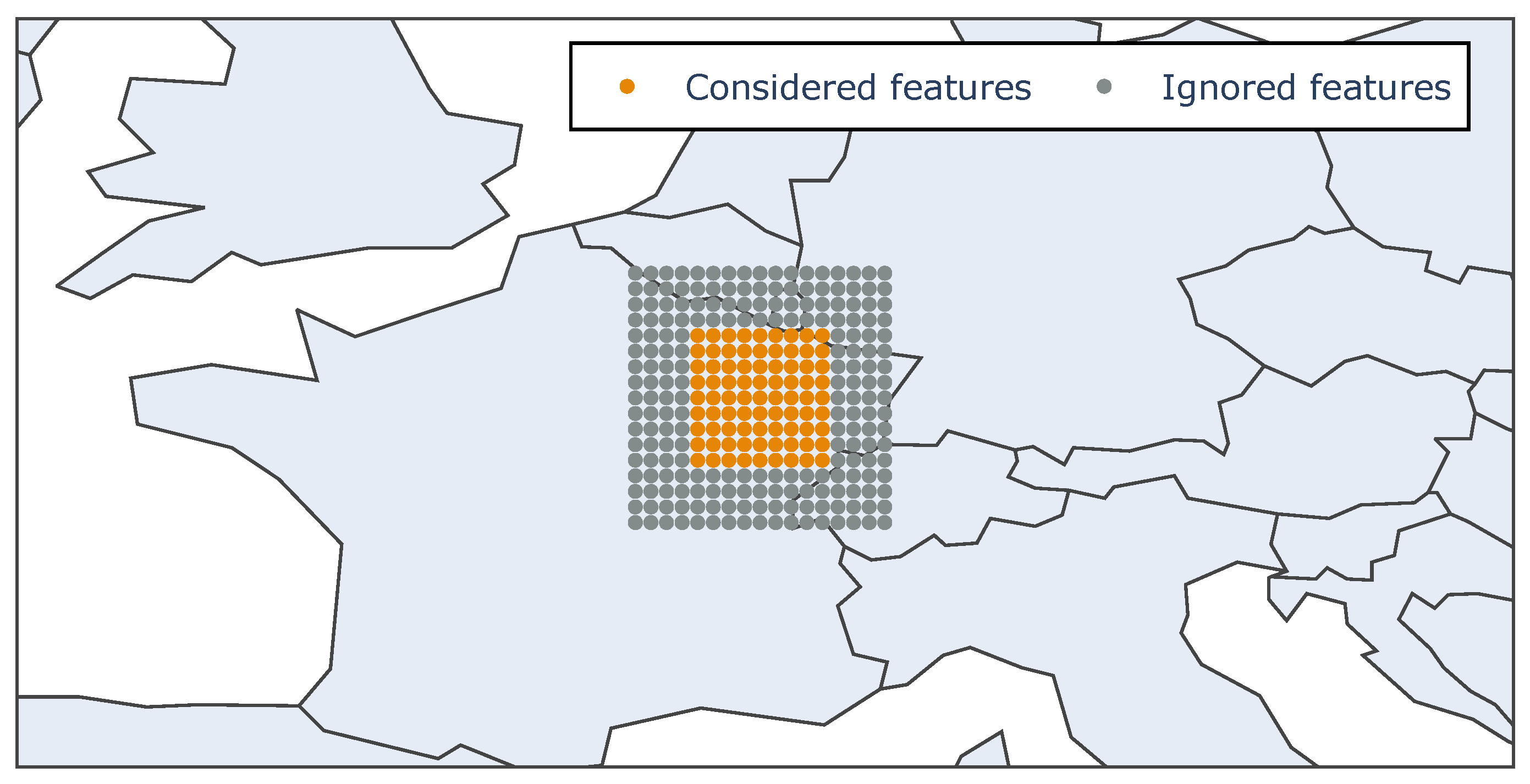
Additionally, to change the whole grid size, the number of features considered from the grid can also be reduced. For each incremental square grid, alternative models can be trained using a subset of features belonging to the perimeter of the forecast map or features relative to the main wind directions (one for each cardinal point), as shown in Figure 8.

6. Evaluation

This section presents an evaluation of the wind power forecasting model on the “La Haute Borne” wind farm. The proposed spatio-temporal neural network was trained and evaluated on all four turbines, identified as R80711, R80721, R80736, and R80790, considering lead times up to 90 h.

The model is evaluated with respect to both the spatial and operational input features. To evaluate the spatial input features, different map sizes and reduced maps are analyzed, while for the operational input features the SCADA data is considered. All evaluations are quantified using the same set of error metrics, which are therefore introduced in the following.

6.1. Evaluation Metrics

The performance of the proposed spatio-temporal neural network for wind power forecasting is evaluated using different metrics. In particular, the Mean Absolute Error (MAE), the Root Mean Squared Error (RMSE), and the Median Absolute Error (MDAE) are considered. Each metric is computed for all lead times individually to provide a better insight into the model prediction errors and, then, normalized by the nominal power of the wind turbines which is 2050 kW. Considering n samples for each lead time t, the error measures can be described as

$${\mathrm{MAE}}_t=\frac{1}{2050n}\sum _{i=1}^n|y_{i,t}-{\widehat{y}}_{i,t}|,$$

$${\mathrm{RMSE}}_t=\frac{1}{2050}\sqrt{\frac{1}{n}\sum _{i=1}^n{(y_{i,t}-{\widehat{y}}_{i,t})}^2},$$

$${\mathrm{MDAE}}_t=\frac{1}{2050}\mathrm{Median}\left(\right|y_{1,t}-{\widehat{y}}_{1,t}|,\dots ,|y_{n,t}-{\widehat{y}}_{n,t}\left|\right),$$

where $y_{i,t}$ is the ground truth wind power and ${\widehat{y}}_{i,t}$ is the proposed model prediction for sample i at lead time t. Finally, to evaluate the overall model performance with respect to a baseline, a Skill Score (SS) is computed with

$${\mathrm{SS}}_t=1-\frac{1}{n}\sum _{i=1}^n\frac{|y_{i,t}-{\widehat{y}}_{i,t}|}{|y_{i,t}-{\overline{y}}_{i,t}|},$$

where ${\overline{y}}_{i,t}$ is the prediction of the XGBoost regressor proposed by Chen et al. [20], widely used in many applications involving regression tasks, including wind power forecasting as done by Phan et al. [21], Cai et al. [22], or Phan et al. [23]. This evaluation metric expresses the percentage of improvement achieved by the proposed model with respect to a baseline, which in this case is the XGBoost regressor. When computing overall performance metrics, each measure is averaged over all lead times.

6.2. Evaluation of Spatial Input Features

Having trained the model with different map sizes and different amounts of features as described in Section 5, the performance on the forecasting task can then be compared. A comparison between full maps, perimeters, and cardinal points is carried out to investigate whether a subset of features covering all wind directions is sufficient to produce accurate forecasts. This preliminary analysis is performed without considering the SCADA data and sub-network in order to focus exclusively on the spatial information included in the forecast maps. The HRES sub-network used for this task counts 11 layers with 64 neurons each and the hyperparameters are selected using a grid search. The analysis is mainly presented for turbine R80721 since representative of the whole wind farm, in order to avoid an excessive amount of similar results for the reader. Nevertheless, a general quantitative overview is provided at the end of the chapter for all turbines composing the wind farm of interest.

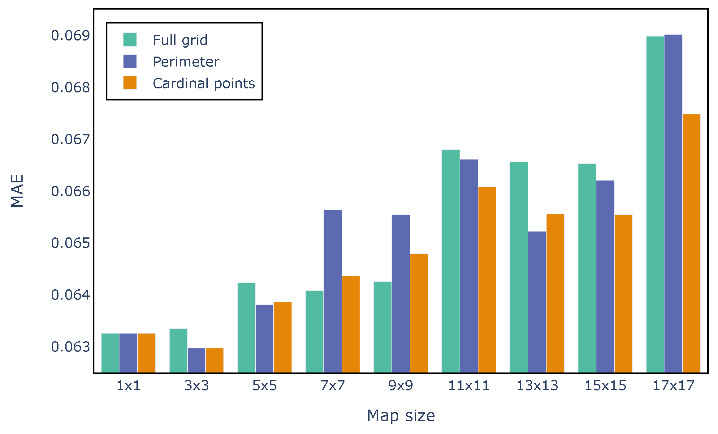
As can be seen in Figure 9, models trained on perimetric or cardinal point features have comparable or even better performances with respect to models trained on full grids. Notably, the $1\times 1$ map size achieves the same MAE in all three scenarios since the input, namely the central pixel, is the same for all models. The lowest overall error is achieved by using perimetric or cardinal point features (which coincide also in this case) with $3\times 3$ grids. Considering full maps is not only slower from a computational point of view but also degrades the model performances for most map sizes, except for the $5\times 5$ and $7\times 7$ maps. Training a one-layer network using $17\times 17$ full grids takes 1:03 min, compared to 37 s achieved by using cardinal point features (speedup of 1.7x).

It is interesting to notice that, when using cardinal point features, the lowest MAE (0.063) achieved using $3\times 3$ grids is only 0.004 lower than the highest MAE (0.067), obtained using the largest map size of $17\times 17$. This means that eight features, one for each wind direction, even when spatially distant from the wind farm, are sufficient to achieve relatively accurate forecasts, thanks to the bidirectional temporal capabilities of the model. In fact, by looking at HRES meteorological forecasts associated with the cardinal points from the past and future of each lead time, the network is supposedly able to model the dynamics of wind and its evolution in time over the entire geographical area.

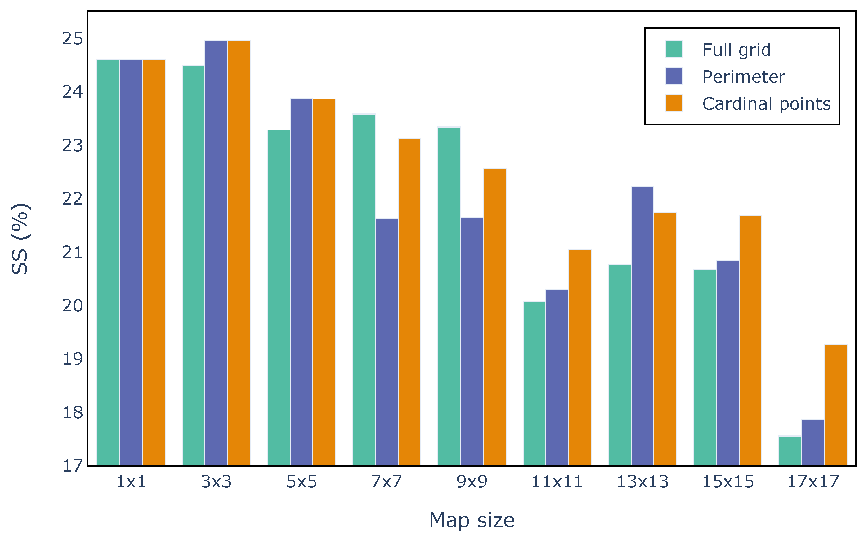
Figure 10 presents the same results in terms of the SS evaluation metric. As a baseline for the score, an XGBoost regression was trained for each lead time selecting as input the whole HRES forecast map. The best results were also achieved by using the $3\times 3$ grid with a SS of 25%, and both perimetric and cardinal point features perform on average better than full maps.

6.3. Evaluation of Operational Input Features

After selecting the optimal grid configuration, namely perimetric/cardinal point features of $3\times 3$ maps, the SCADA data and sub-network were integrated into the training process to produce the final wind power forecasts. This sub-network counts 11 layers with 64 neurons each and considers a window of 24 h of observed historical measurements in order to capture the last daily cycle of the turbine’s operating conditions. Furthermore, in this case, the hyperparameters are selected using a grid search. The whole model takes approximately 30 min to train on CPU for 60 epochs using an Apple M1 employing the augmented dataset described in Section 3 and a batch size of 64. Inference, once the network is trained, takes only a few seconds, making it suitable for real-time forecasting.

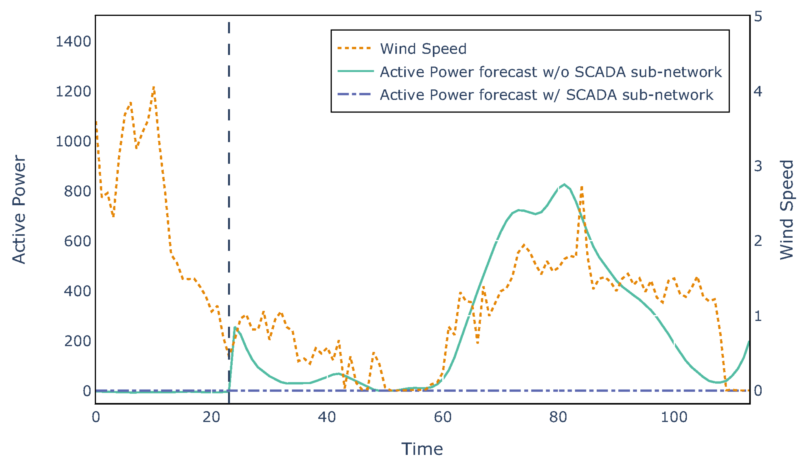
When integrating the SCADA data and sub-network, the model performance for turbine R80721 increased by only 0.005 in terms of SS, since no major failures or inefficiencies occurred during the four years of operation considered for this study. However, it is interesting to notice that without the SCADA component, the network always predicts a non-zero active power based on the wind speed, even when the turbine is shut down and outputs no power. When the operating conditions of the turbine are considered by means of the SCADA sub-network, instead, the model is able to successfully predict a zero active power. An example of such a scenario is provided in Figure 11.

6.4. Comparison to Benchmarks

In order to compare the performance of the spatio-temporal neural network with benchmark algorithms, the MAE for all lead times was computed for the proposed model, linear regression, the XGBoost regression, and another promising neural architecture, namely a Convolutional LSTM (ConvLSTM) network [24]. 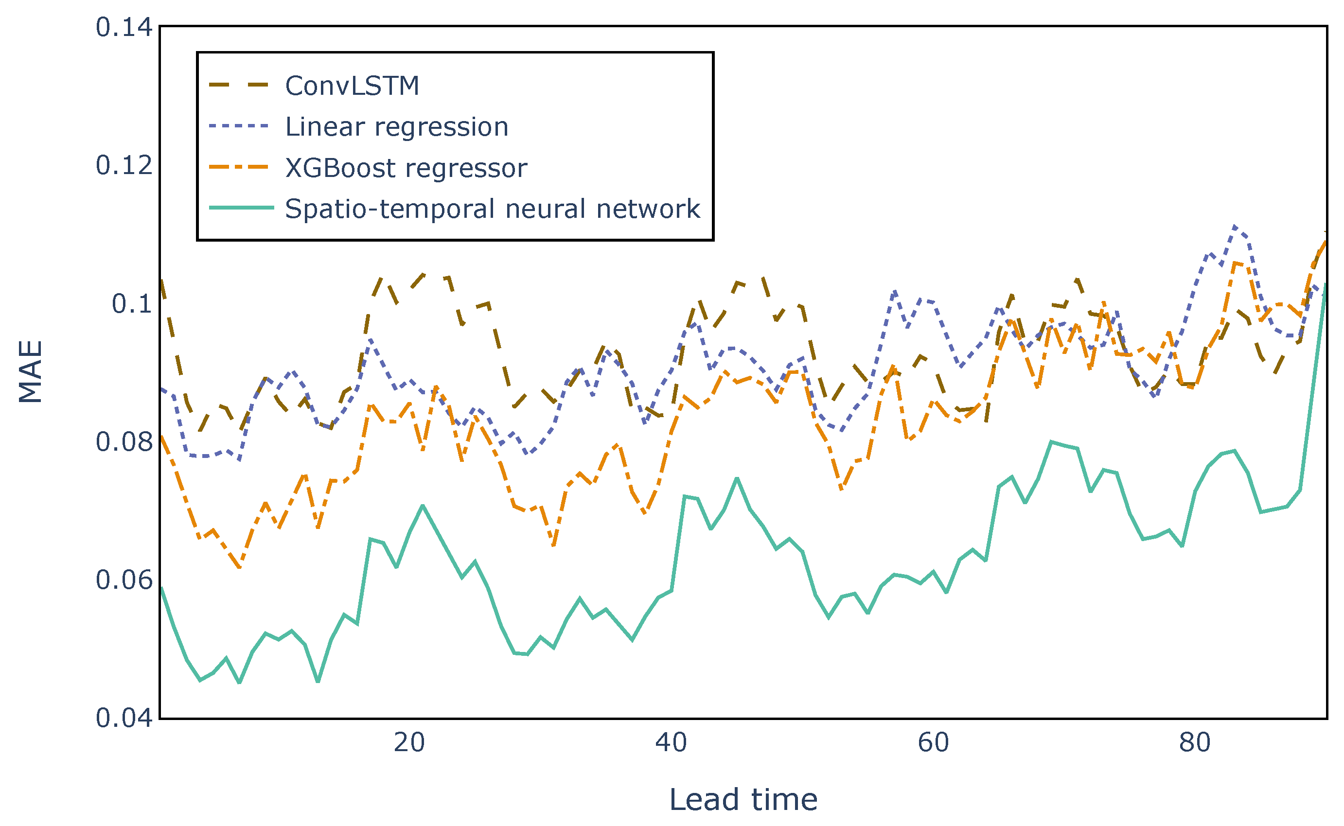For all benchmarks, a separate model was trained for each lead time providing as input the whole $17\times 17$ forecast map. As shown in Figure 12, the network outperforms the other regression models overall, achieving an error of 0.044. It is interesting to note that the MAE for the last two lead times (89 and 90) of the spatio-temporal network increases and becomes comparable to the other models. This is probably due to the fact that the bidirectional neural architecture has no access to information from the future and, therefore, produces worse results. Moreover, forecasting wind power with lead times close to 90 h in the future is a challenging task in itself, which is confirmed by the fact that the temporal resolution of NWP forecasts decreases. Notably, even though the HRES maps are in the form of images, the spatio-temporal neural network outperforms a more complex architecture based on Convolutional LSTMs both in terms of time and prediction error. In fact, the proposed network requires 30 min to train for 60 epochs, while the ConvLSTM takes 300 min, achieving a speedup of $10x$. In addition, the lead time errors of the ConvLSTM are always higher than the proposed network, probably due to the excessive complexity of the model when dealing with small map sizes.

Looking at Figure 12, it can be seen that the errors follow a daily pattern, with low MAEs during morning lead times and high MAEs during evenings. For example, during the first daily cycle (lead times from 1 to 24), the minimum error MAE (0.044) corresponds to 4 AM forecasts and the maximum (0.067) to 9 PM predictions, with a difference of 0.023 during a span of 24 h. This result is in line with the strong diurnal cycle of wind forecasts resulting in usually lower predictability from the afternoon up to midnight due to the presence of atmospheric convection [25,26]. Even though there is a daily cycle, the lead time errors follow an overall increasing trend correlated to the temporal distance from the midnight forecast origin.

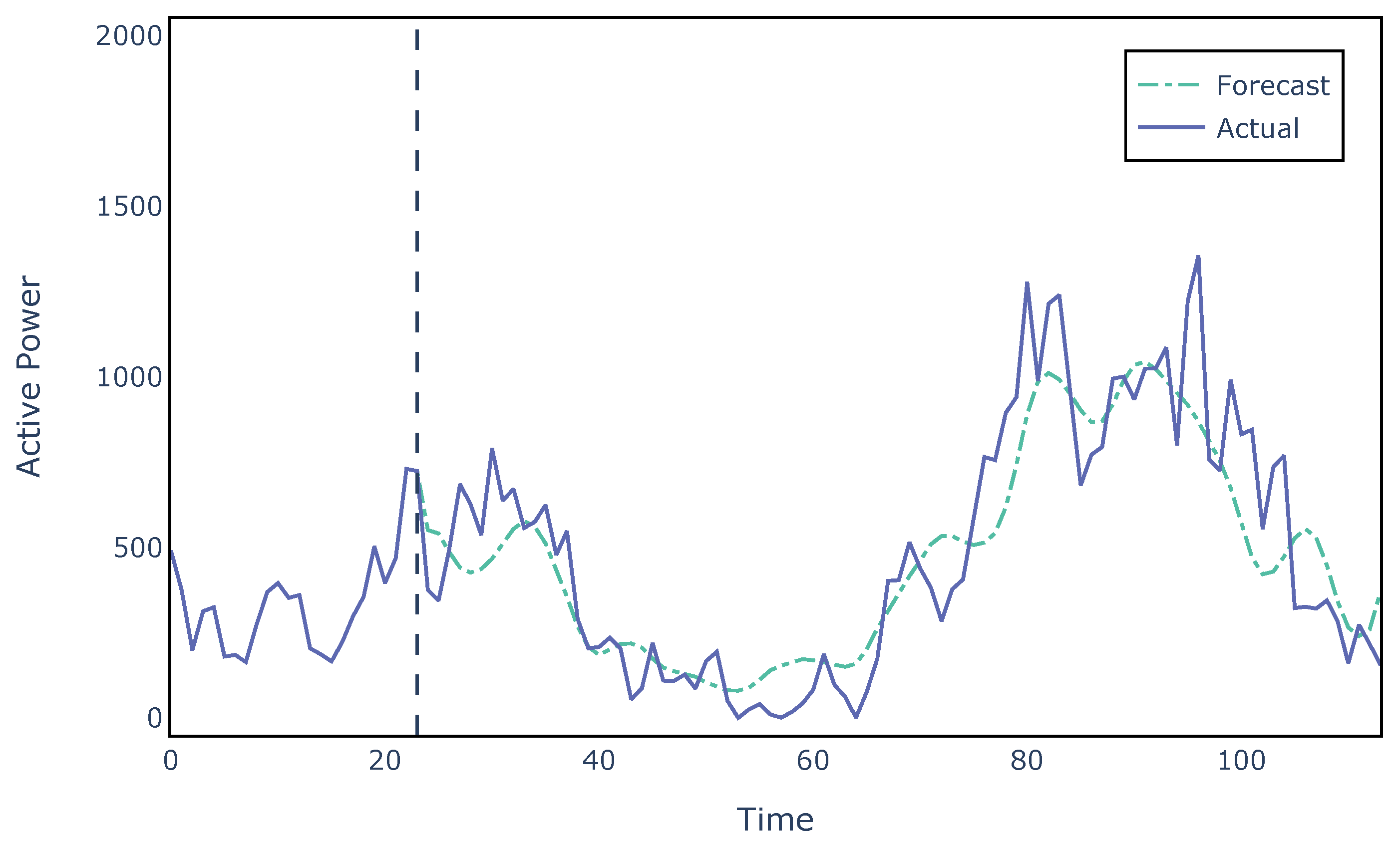
An example of wind power forecasts produced by the proposed spatio-temporal neural network is presented in Figure 13. It is evident that the model is unable to predict the fluctuations of higher frequency which are hard to capture, especially when the meteorological data are not specific to the wind farm location but rather to a regular grid surrounding it. Nevertheless, the network is able to predict the general trend of the active power produced by the wind turbine up to almost 4 days in the future.

Finally, in order to provide a general quantitative analysis for the whole wind farm,

Table 1. The table presents the prediction errors in terms of MAE, RMSE, and MDAE averaged over lead times, together with the overall SS, for all four wind turbines.

Turbine ID	MAE	RMSE	MDAE	SS
R80711	0.078	0.121	0.045	0.236
R80721	0.063	0.103	0.035	0.255
R80736	0.066	0.109	0.036	0.265
R80790	0.072	0.118	0.040	0.248

presents the evaluation metrics computed for all four wind turbines. The scores are comparable among turbines and achieve an average SS of 0.251, meaning that the proposed spatio-temporal neural network performs $25.1\%$ better on the whole wind farm with respect to an XGBoost regressor trained on the same data.

7. Conclusions

This paper proposed a multi-modal spatio-temporal neural network for multi-horizon wind power forecasting considering a lead time of up to 90 h. In particular, the model combined high-resolution NWP forecast maps with turbine-level SCADA data, and explored how meteorological variables on different spatial scales together with the turbines’ internal operating conditions impact wind power forecasts.

The spatial analysis of HRES maps showed that a subset of features associated with all wind directions can produce more accurate forecasts with respect to full grids and reduce computation times. In this way, when no regular grid data are available in the immediate surrounding of the wind farm, it is still possible to forecast wind power by considering features corresponding to the main wind directions, even if spatially distant.

The spatio-temporal neural network was compared to a linear regression, the XGBoost regressor, and a ConvLSTM network, subsequently outperforming them across all lead times. More specifically, the proposed model improved the XGBoost baseline with an average skill score of 25.1%.

For future work, it is of interest to extend the analysis to other wind farms where more anomalies, failures and downtimes have occurred and are reported in a maintenance log. In this way, the network can model these scenarios and improve the wind power forecasts based on the turbine’s operating conditions. Moreover, it would be of interest to train the proposed neural network on other wind farms that experience similar wind conditions to understand whether the same subset of NWP maps, namely $3\times 3$ cardinal point features, leads to the best results, or if it depends on the topology of the area surrounding the wind farm.