Abstract
The proliferation of inverter-based distributed energy resources (IBDERs) has increased the number of control variables and dynamic interactions, leading to new grid control challenges. For stability analysis and designing appropriate protection controls, it is important that IBDER models are accurate. This paper focuses on the accurate estimation and parameter calibration of DER_A, a recently proposed aggregated IBDER model. In particular, we focus on the parameters of the reactive power–voltage regulation module. We formulate the problem of parameter tuning as a non-linear least square minimization problem and solve it using the Levenberg–Marquardt (LM) method. The LM method is primarily chosen due to its flexibility in adaptively selecting between the steepest descent and Gauss–Newton methods through a damping parameter. The LM approach is used to minimize the error between the actual measurements and the estimated response of the model. Further, the computational challenges posed by the numerical calculation of the Jacobian are tackled using a quasi-Newton root-finding approach. The proposed method is validated on a real feeder model in the northeastern part of the United States. The feeder is modeled in OpenDSS and the measurements thus obtained are fed to the DER_A model for calibration. The simulation results indicate that our approach is able to successfully calibrate the relevant model parameters quickly and with high accuracy, with a total sum of square error of .
1. Introduction
The growing penetration of inverter-based distributed energy resources (IBDERs) has provided opportunities for a sustainable and smarter renewable-rich smart power grid (RRSPG). In fact, renewable energy sources (RESs) can supply up to load demand in today’s power systems. In traditional electric grids, system characteristics were based on conventional generators, such as synchronous machines. However, with advancements in control flexibility, DC-AC conversion, and power electronics, the penetration level of IBDERs in RRSPG has increased to the point where their influence on system characteristics can no longer be disregarded. The IBDERs impact includes, but is not limited to, peak demand [], voltage control [], hosting capacity [], and dynamic performance []. In contrast to conventional synchronous generators, which are governed by physics (principles such as flux linkage, etc.), the behavior of IBDERs is regulated by power electronics and control algorithms. Due to these features, IBDERs have the ability to perform a range of functions, such as high/low voltage ride through (LVRT/HVRT) and primary frequency response through active power–frequency control. The functional and structural differences/features are described in standard IEEE 1547-2018, which discusses operation and stability for IBDERs [].
Each IBDER possesses unique characteristics, and even if the underlying electronic systems are identical, their dynamic behavior may vary depending on their location in the feeder or on the variance between the medium voltage network and the low voltage network. Ideally, every individual DER would be modeled to precisely represent its dynamic behavior, but due to the growing number of IBDERs, this becomes computationally challenging. Moreover, many IBDERs are usually placed behind the meter, adding to the uncertainty and complexity of modeling. The aggregation of IBDERs provides an adequate approximation of the collective behavior of smaller IBDERs, which offers sufficient detail for utilities to conduct studies on transient stability, grid planning, and the system’s performance at the point of interconnection (POI) [,]. The authors in [] show that aggregators do add value to the power system in the long term, though the regulation should be improved. Despite the necessity of accounting for the aggregated behavior of IBDERs, industry research shows that in approximately one-third of cases, IBDERs are modeled through negative loads in bulk system dynamic studies []. This could be a result of one or more of the following []:
- Lack of well-defined, well-validated model for IBDERs.
- Lack of widely accepted model for IBDERs and their parameters.
- Little information about IBDERs, especially at low voltage levels.
- Lack of accepted approaches for IBDER aggregation.
- Lack of widely accepted approach for parameter calibration of IBDERs.
Significant efforts have been made over the past decade to define a generic model for IBDERs. The Western Electricity Coordination Council (WECC) first proposed pvd1 to account for the aggregation of IBDERs [,,]. However, pvd1 lacks the ability to mimic several new functionalities, such as LVRT/HVRT, active power–frequency control, and reactive power–voltage control introduced by the recently updated IBDER standard IEEE Std 1547-2018 and California Rule 21. Other generic models, such as regc_a, reec_a, repc_a, lhvrt and lhfrt, mostly intended for large-scale PV plants, are very complex with 5 modules, 121 parameters, and 16 states []. Therefore, a simpler model is needed that can mimic the new features of modern inverters as outlined in IEEE 1547-2018.
WECC introduced DER_A [,], a time-domain positive-sequence model to represent the combined dynamic behavior of up to a hundred IBDERs, which can account for both legacy and modern IBDERs. DER_A was subsequently attached to the WECC composite load model for representing aggregated IBDERs [] and is now included as a library model in major positive sequence simulation software tools []. Overall, DER_A has significantly reduced the order of 2nd generation RES models by decreasing the number of parameters to 48, i.e., 1/3 of the number of parameters in a full 2nd generation model. Despite a significant reduction in the number of parameters in this model, the challenge of tuning these parameters remains significant. It is crucial that these parameters accurately reflect the actual behavior of IBDERs without imposing any limitations on their capabilities.
The DER_A model development and parameter tuning studies in the literature are shown in Figure 1. A comprehensive study on the DER_A model is carried out in [] by applying small and large disturbances of voltage and frequency using various commercial simulation platforms; however, the focus of the study is limited to verifying the accuracy of the model response []. Nevertheless, Ref. [] can be considered a suitable benchmark for further analysis and parameterization studies of the model. Parameterization studies are mostly focused on the partial trip setting of the model []. Authors in [] derive a set of generic parameters with a focus on the parameterization of the fractional tripping module and assume generic settings for the rest of the parameters. Authors in [] obtain the voltage tripping parameters of DER_A using dynamic Monte Carlo simulations, but they do not address other model parameters. Nevertheless, the proposed DER_A model is relatively new and there is a lack of extensive research. Further, most of the studies address the parameterization of fractional tripping parameters while assuming default values for other parameters. However, as mentioned in [], appropriate model selection with inappropriate parameters is a very critical issue. Therefore, it is extremely important to address other parameters of the model, especially voltage control parameters.
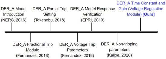
Figure 1.
Comparison of DER_A parameter calibration in the literature [,,,,,] and our proposed method.
This paper addresses the above challenge by investigating the problem of the parameterization of aggregated models of IBDERs, focusing on mostly unexplored parameters of the model that cannot be specifically determined from the system characteristics. A framework based on Levenberg–Marquardt (LM) is proposed for IBDER parameter calibration. The proposed LM algorithm is designed to minimize the error between the measurements and model response by adaptively selecting between the steepest descent method and the Gauss–Newton method using a damping parameter. To this end, an optimization-based approach is proposed, relying on minimizing the square error in a nonlinear fashion. Generally, in such studies, the calculation of the Jacobian can become a bottleneck—(1) many commercial simulation platforms do not provide internal states crucial for Jacobian calculation; (2) further, numerical calculations of Jacobian can be very time consuming and computationally expensive. Our proposed framework addresses the challenges of the Jacobian calculation using a quasi-Newton root-finding approach, reducing the computation time simultaneously. A real-world RRSPG feeder with considerable PV penetration [] was selected for numerical validation. The feeder was modeled in OpenDSS, and measurements were obtained for calibration. These measurements were then fed to the simulated DER_A model developed in MATLAB to generate the response. The error between modeling the behavior and the measurement forms the basis of the parameter calibration using the LM method. The simulation results show a considerable match between the measurement and the model response with calibrated parameters. The estimation errors also confirm the successful calibration of targeted parameters. Correctly tuned models play an important part in DER_A benchmarking and testing, which is currently beyond the scope of this paper. The contributions of this work can be summarized as follows:
- We provided a comprehensive review of IBDER model estimation and calibration.
- We developed an approach for calibration of aggregated IBDER models in RRSPG, which can be generalized to any model and integrated with any simulation platform.
- We addressed grid reliability issues imposed by inaccurate aggregated IBDER models by proposing a new optimization-based algorithm. The proposed Levenberg–Marquard method minimizes the error between measurements and the simulated response of aggregated IBDER model by adaptively selecting between the steepest descent and the Gauss–Newton using a damping factor.
- We addressed the computational challenges of numerical calculation of the Jacobian through a quasi-Newton root-finding approach.
- We validated the developed algorithm using the real system feeder modeled in OpenDSS. For DER_A response to an emulated fault, the d-axis and q-axis current values were used as measurements, while the measured terminal voltage and frequency were taken as the model response. We developed and simulated DER_A employing the LM-based proposed method in MATLAB.
- We proposed a general framework to integrate the model parameter calibration method of the aggregated IBDER model into industrial dynamic simulators for RRSPG. Specific model parameters selected for calibration in this work can be extended to other parameters easily.
The rest of the paper is organized as follows: Section 2 reviews the DER_A model and its parameters. Section 3 formulates the problem of parameter estimation, while Section 4 discusses the proposed method in detail. Section 5 explains the numerical simulations carried out to test and validate the proposed method, and, finally, Section 6 concludes the paper and sets the direction for future works.
2. Review of the DER_A Model
Over the last decade, various attempts have been made to develop aggregated inverter-based generation (IBG) models for transmission planning and stability studies. To this end, DER_A was introduced by WECC in compliance with interconnection standards []. It was added as a positive-sequence load at the end of the feeder; it can be used either as a standalone or aggregate, and is a simplified version of previous models. The DER_A model has fewer states and parameters compared to other generic models, yet is inclusive of modern inverter features. Figure 2 shows the detailed block diagram of DER_A, which includes the following features:
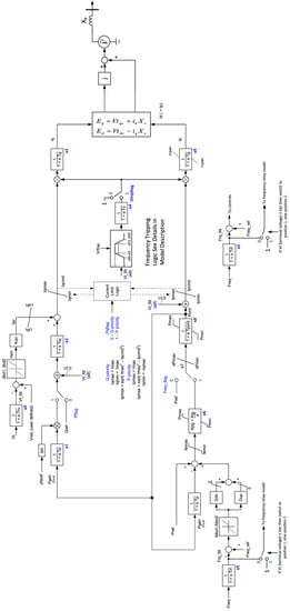
Figure 2.
Block diagram for the DER_A model version A [].
- Active power–frequency control;
- Frequency tripping logic input;
- Reactive power-voltage control;
- Active–reactive current priority logic;
- Fractional tripping;
- Voltage source representation.
Among all the modules, the partial tripping module has attracted the most attention, as the partial tripping parameters determine the behavior of the aggregated DERs in a direct way. The module emulates the aggregated behavior of DERs along the feeder under abnormalities in the grid, such as low- or high-voltage scenarios. The ratio of legacy inverters to modern inverters, corresponding time settings, and locations along the feeder collectively determine the values of and other parameters of the tripping module. The North American Electric Reliability Corporation (NERC) has recommended a few options to roughly determine voltage break points (, , , ), though it is encouraged to use engineering judgment and sensitivity analysis as well []. The NERC guideline is mostly considered as a starting point, and probes for alternate methods are underway. Authors in [] randomly distributed DERs along the feeder and characterized the tripping module by extensive simulations. A dynamic study and quasi-static simulation are conducted in [] to explore the low voltage dynamic response of the aggregated model. It is shown that the obtained behavior is significantly different from the response of default values provided by NERC []. The parameters of a generic PV model can be divided into four categories []:
- Parameters in accordance with grid connection requirements (GCRs);
- Parameters that are highly manufacture dependent;
- Parameters that do not affect the simulation results;
- All other parameters.
Such a classification might be helpful for areas with specific grid connections, such as Dutch Netcode, which requires fast fault current for IBGs. However, restricted requirements often limit the boundaries of some parameters. However, the U.S. IEEE 1547 and California Rule 21 are voluntary industry standards and have no inherent authority. While the standards recommend certain features, such as voltage regulation, they are still quite flexible and allow the governing authority to configure these capabilities as they see fit for meeting the interconnection requirements. Note that manufacture-dependent parameters are not particularly useful in the case of aggregating several hundred DERs behind the meter.
To the best of the authors’ knowledge, there are no other studies other than [] that address the parametrization of non-tripping parameters of DER_A. The authors in [] used sensitivity analysis and literature research to assign values to unknown parameters. Sensitivity analysis has been used as a primitive identifiability test for other problems, such as composite load model identification [], although it is acknowledged that sensitivity analysis can be performed in a more intrinsic manner by using optimization-based tuning. The determination of other model parameters, such as time constants and gains, has not been discussed thoroughly, and default values are mostly considered in the literature. These parameters are the main focus of the paper.
3. Problem Formulation
In this paper, we focus on unaddressed time constants and gain parameters of the DER_A model. These include parameters of the voltage regulation module—time constant T_rv, proportional control gain K_qv, and lower and upper deadbands dbd_1 and dbd_2, respectively. We adopt a more structured and reliable approach based on optimizing the estimation error for parameterization. The proposed tuning framework can be easily adapted for other parameters of the model as well.
The problem of parameter tuning is formulated as a least-squares problem. Here, the desired outputs or true measurements of the sub-system model are used as the reference. These desired outputs are the d-axis and q-axis currents ( and ) of aggregated DERs, as shown in Figure 2. Considering DER_A model as a grey box system, the output is written as follows:
where u is the input vector comprising the terminal voltage and frequency F, p represents the uncalibrated parameters, and f denotes the nonlinear function that maps the input vector to the estimated output vector with the specified parameters. The input vector along with the aggregated active and reactive power outputs of DERs, P and Q, can be measured from the field or the simulator modeling the whole feeder. The terminal currents of dq-axes are calculated as
Note that, here, is the terminal voltage and . By feeding the input vector to the model aggregator f, an estimation of outputs is obtained that can be used for the parameter tuning process. This approach is called signal playback and has been used in a variety of model validation and calibration applications in the literature [].
Problem Statement: The problem of tuning the DER_A parameters based on the measurements is a nonlinear least-squares problem. Here, the unknown parameters of aggregated DER model p are calibrated by minimizing the error between the measurements taken from the field and the estimated response of the model. The problem is mathematically formulated as
4. Proposed Solution Approach
4.1. Levenberg–Marquardt Method for Parameter Tuning
To solve the above problem, we propose to implement the Levenberg–Marquardt (LM) method. The LM was first introduced by Levenberg [] and then by Marquardt [] independently. It is one of the well-known and most successful nonlinear least-squares methods due to its easy implementation and fast convergence characteristics. LM exhibits adaptive behavior by incorporating a damping factor into its step-size calculation formula. This factor is increased if LM fails to reduce the square error, and decreased otherwise. In a sense, LM can be defined as a mixture of the Gauss–Newton and steepest descent methods []. Because of the inherent flexibility and efficiency, LM is used to estimate the unknown parameters of the DER_A model. The LM method creates an affine approximation of f around p as
where f is the function that maps parameters p and inputs vector u to an estimation of measurements . Here, is the Gauss–Newton step and J is the Jacobian of f. Like other nonlinear optimization methods, LM tries to estimate a series of parameter vectors iteratively, where k denotes the iteration step. The objective is to lead the parameter vector closer to its optimal value at each iteration so that the error between the actual measurements and the estimated measurements ultimately becomes zero or close to zero. An incremental step is added to the parameter vector for updates, and the 2-norm of estimation error is minimized as
where is the measurement vector, and is the estimation error. Without loss of generality and for the simplicity of representation, we drop the input vector u from the equations. Note that the measurement time series is treated as a batch in the above framework. To minimize the estimation error, the derivative of (6) with respect to p is set to zero, which leads to the following normal equations:
where is first-order approximation of Hessian of error, refers to the direction of the steepest descent and denotes the transpose operation. To adaptively switch between the steepest descent and the Gauss–Newton, a damping parameter is introduced, and the augmented normal equations are
Small values of result in a Gauss–Newton update, while larger values result in the steepest descent update. Initial values of are usually set as large so that the step is small in the steepest descent direction. By approaching the optimal point, becomes smaller, and therefore, LM leans toward the Gauss–Newton method. In each iteration of LM, the step is calculated by solving (8). If the updated parameter vector cannot reduce the error further, the damping parameter is increased, and the iteration continues until an accepted step is found that reduces the error. The details of the proposed approach are presented in Algorithm 1. The algorithm stops if it either reaches the predefined maximum number of iterations or meets the stopping criterion defined below:
The parameters , and are user defined. Note that the maximum number of iterations should be set to be large enough for the algorithm to converge to an acceptable level of accuracy.
| Algorithm 1: Proposed DER_A parameter calibration with Levenberg–Marquardt method. |
Input: Measurement vector , mapping function , and initial parameter estimation . Output: A which minimize . Begin: ; ; ; ; ; ; found:= ;  |
4.2. Quasi-Newton Method for Jacobian
The numerical calculation of Jacobian is challenging and we address this problem using a quasi-Newton root-finding approach. The Jacobian J can be approximated numerically using either forward or central difference. The forward difference is as follows:
where is an all-zero vector except for the jth element which is a very small positive number h. Although the finite difference method is an efficient method to calculate the Jacobian, it becomes computationally expensive, especially if the number of parameters is large. To address this problem, the quasi-Newton root-finding method is used to evaluate the Jacobian only at the first iteration and subsequently implement a -1 Jacobian update []:
The Jacobian approximation using (12) may deteriorate eventually, necessitating a re-evaluation of the Jacobian after several iterations. Hence, at the first iteration, at every iteration, and at iterations where (i.e., the step gets rejected), the Jacobian is re-calculated using finite differences using (11). Note that the gradients can also be calculated analytically; however, this requires having an accurate representation of the model, which may not be readily available.
To summarize, this paper implements the LM method to calibrate unknown time constant and gain parameters of the DER_A reactive power–voltage regulation module. In this context, the measured fields are d-axis and q-axis current and , respectively, and the mapping function f is the output of DER_A when the measured terminal voltage and frequency feed it. The next section discusses the results of our approach.
5. Simulation Results
The proposed method is validated on a real distribution feeder located in the northeastern part of the US, which includes a MW customer-owned PV []. The system topology is shown in Figure 3. The feeder specifications are listed in Table 1.
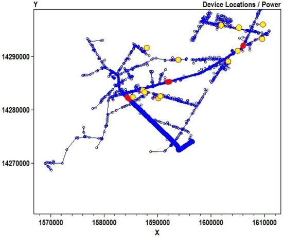
Figure 3.
Topology of the test system with regulators (red) and PV buses (yellow) [].

Table 1.
Test system specifications.
5.1. Modeling of Actual Distribution System
The model of the distribution feeder shown in Figure 3 is developed in OpenDSS []. The voltage profile of the test feeder without any DERs is shown in Figure 4. To emulate the fault condition, a voltage sag is induced at a substation to observe the aggregated behavior of the DERs. The voltage sag waveform is generated as
where is the voltage sag level, cycles is the sag duration, s is the recovery time, and is the ramp recovery starting level []. This waveform is used as an input to the voltage source at a substation to simulate a three-phase fault in the transmission system.
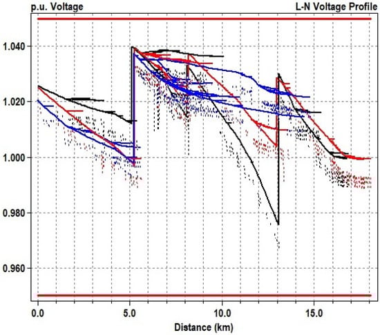
Figure 4.
Voltage profile of the test feeder without any DER and with balanced loads. Phases A, B, and C are denoted in black, red, and blue, respectively. The dotted lines mark the voltage magnitude on the secondary side of the transformers [].
Traditionally, distribution systems are simulated in steady-state or quasi-static environments using multiple snapshots of power flow. However, the high penetration of IBGs requires dynamic simulations. To this end, OpenDSS dynamic simulation is used to study the response of the feeder to the emulated fault in (13). In order to calculate the active and reactive power of aggregated DERs, the simulations are run twice—with and without PVs. The net difference makes up for the DER response as shown in Figure 5. Finally, the terminal currents of dq axes are calculated using (2).
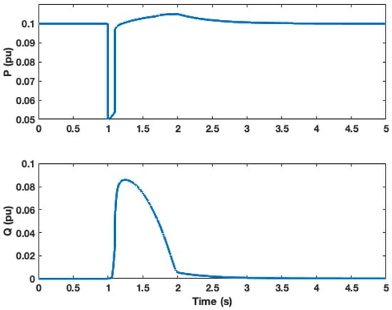
Figure 5.
Aggregated real and reactive power of PVs obtained from OpenDSS.
5.2. Calibration Results for DER_A Model
We assume that all inverters have the capability to return to their normal operation after the fault has been cleared, i.e., . The rest of the parameters are selected based on IEEE Std. 1547-2018 (Category III) in []. For target parameters, we used values listed in the “Before Calibration” column based on NERC guideline [], as shown in Table 2.
Table 2.
Results before and after parameter calibration.
The DER_A block diagram is implemented in MATLAB Simulink. The signal playback method is used for the estimation and calibration process. Figure 6 shows the terminal voltage and frequency fed to the model. Estimated terminal currents and are considered the model outputs. The augmented vector of terminal current values for all the simulation time is considered as , where y is the measurement obtained from OpenDSS, and is the parameter vector.
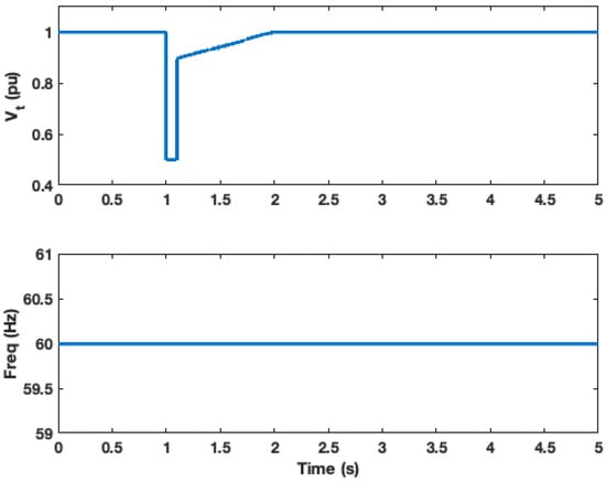
Figure 6.
The input signals feeding the DER_A.
The proposed LM framework developed in Section 4 is implemented in MATLAB to calibrate the parameters. Table 2 summarizes the calibration results. The results are validated on a real-world feeder through the following steps: first, measurements are obtained from the OpenDSS software, which is used to model the feeder. These measurements serve as the baseline. Second, these measurements are fed to the simulated DER_A model developed in MATLAB to generate the system response. Figure 7a,b show the model estimation before and after the calibration process and compares them to the field measurements. While there are significant disparities between the model estimations and the measurements prior to calibration, it is seen that the calibrated outputs match the measurements perfectly. The error between the measurements and the estimated response of the model is minimized using our proposed approach. In the beginning, the sum of the squared error is , which is reduced to at iteration 12, thus validating our approach.
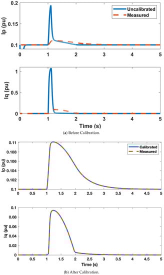
Figure 7.
Measurements vs. model response (a) before and (b) after calibration.
It is worth noting that despite using default parameter values as the initial parameter values as defined by the NERC guidelines, the model estimation is highly inaccurate. This shows that the parameters that typically do not gain significant interest from researchers can significantly influence the model estimation and should not be ignored.
Figure 8 illustrates the calibration progress. It is observed that the step size, or rate of change, is initially large, but as the optimization process approaches the optimal point, it gradually decreases. This validates that the LM behaves as the steepest descent in the beginning and then leans toward the Gauss–Newton.
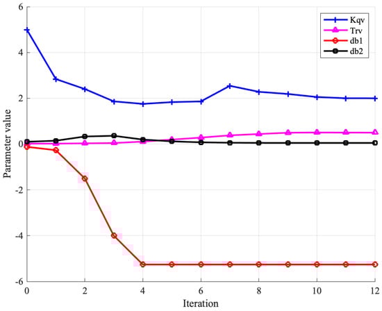
Figure 8.
Progress of the parameters estimation process.
Figure 9 shows the estimation error, i.e., the residuals between the measurements and model estimation with the tuned parameters. It is observed that the errors are significantly small, and as expected, most of the errors are concentrated during the dynamic period. Figure 10 further illustrates the sum of squared error as the calibration progresses. Similar to the rate of change of parameters shown in Figure 8, it is observed that the error is high at the beginning and gradually goes toward 0 as it approaches the optimal point.
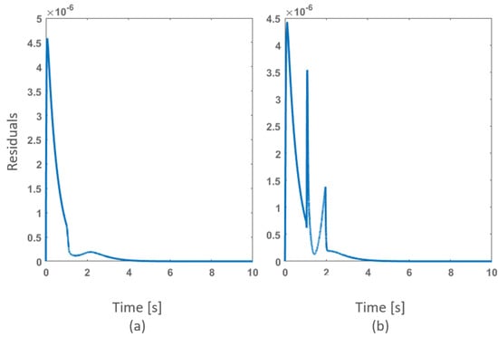
Figure 9.
Estimation residuals for (a) and (b) .
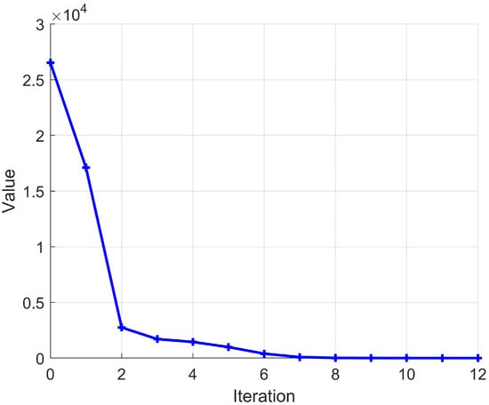
Figure 10.
The sum of squared error over each step of the iteration during the calibration process.
It is noted here that we performed our simulations using two traditional methods—the steepest descent and the Gauss methods; however, they did not converge.
5.3. Discussions
It is worth mentioning that at first, the calibration process diverged, and reasonable values could not be obtained. It was observed that the instant gain and the time constant diverged to negative values; hence, we set limits for these parameters as , , and . To implement these conditions, the limits were tested with in the LM algorithm.
After setting these limits, we ran the experiments again, and the calibration converged to the values given in Table 2. It is observed that the final value of was not reasonable. Further investigation revealed the following: for the particular voltage input given in (13), the lower band is not being triggered, and therefore, the calibration for this parameter diverges. In other words, is not sensitive to this particular input. To address this issue, we recommend another test, such as voltage swell []. This is, however, out of the scope of the paper.
The developed LM-based calibration technique can be used for a broad range of both commercial and industrial applications. This is because the method is entirely numerical in nature and relies solely on the model outputs. As a result, the proposed technique can be utilized with any other model or simulation platform. It can be implemented without any need for model details and internal states. To do this, one can simply write a custom-defined script for currently available dynamic simulators, such as Siemens PSS®E, PowerWorld and DigSILENT PowerFactory, which have already included DER_A in their libraries. Further, our proposed method is not time consuming, and hence can be used as a preprocessing step prior to being utilized in real-time setup.
There are two limitations to our approach. First, the Levenberg–Marquardt algorithm is sensitive to the damping parameter—a small parameter may lead to slow convergence, while a large parameter may lead to a local minimum. Second, finding accurate values for user-defined , , and may pose some challenges.
6. Conclusions and Future Works
With increasing challenges of power system operation and control with DERs, this paper investigated the parameter calibration of DER_A, a recently proposed aggregated DER model. We focus on tuning time constants and gain parameters, specifically the T_rv, K_qv, dbd_1 and dbd_2 parameters in the reactive power–voltage control module. These non-tripping parameters of the model have a huge impact on the model response and are hence considered for tuning, which has not been done previously. Through our experiments, we observe that the NERC guideline can only serve as a starting point for parameterization, and further calibration is extremely necessary based on actual measurements. To this end, we propose an optimization-based nonlinear least-squares problem to calibrate the parameters by minimizing the error between the field measurements and the estimated response of the model. We implement the Levenberg–Marquardt approach that solves the nonlinear least-squares problem by adaptively choosing between the steepest descent and the Gauss–Newton method. The challenge of accurately and quickly calculating the Jacobian is addressed by using a quasi-Newton root-finding approach. We validate our approach on a real-world feeder with considerable PV penetration. The error between the model behavior and measurement forms the basis of parameter calibration for the Levenberg–Marquardt method. The simulation results indicate a strong correspondence between the model response and the measured data, demonstrating the successful calibration of the relevant parameters. The low estimation sum of square error of at the final iteration further supports the efficacy of the calibration process. The proposed method has several advantages: it is measurement based, entirely non-intrusive, and can be implemented across any platform without the need for model details and internal states. In the future, we will extend our study to evaluate other parameters (low-voltage and high-voltage cutout breakpoints) of the model, as well as different grid conditions and disturbances.
Author Contributions
Conceptualization, A.S.; Formal analysis, A.F.; Writing—review & editing, S.B. All authors have read and agreed to the published version of the manuscript.
Funding
This research received no external funding.
Acknowledgments
Authors would like to acknowledge partial support available from the US National Science Foundation and the US Department of Energy to conduct this work.
Conflicts of Interest
The authors declare no conflict of interest.
Abbreviations
The following abbreviations are used in this manuscript:
| Gauss–Newton step | |
| estimation error | |
| F | frequency |
| d-axis and q-axis currents | |
| J | Jacobian |
| k | iteration step |
| predefined maximum number of iterations | |
| , | user defined stopping criteria |
| p | uncalibrated parameters |
| P | aggregated active power output of DER |
| Q | aggregated reactive power output of DER |
| u | input vector |
| damping parameter | |
| terminal voltage | |
| estimated output vector | |
| field measurements |
References
- Haghdadi, N.; Bruce, A.; MacGill, I.; Passey, R. Impact of distributed photovoltaic systems on zone substation peak demand. IEEE Trans. Sustain. Energy 2017, 9, 621–629. [Google Scholar] [CrossRef]
- Murray, W.; Adonis, M.; Raji, A. Voltage control in future electrical distribution networks. Renew. Sustain. Energy Rev. 2021, 146, 111100. [Google Scholar] [CrossRef]
- Cicilio, P.; Cotilla-Sanchez, E.; Vaagensmith, B.; Gentle, J.P. Transmission Hosting Capacity of Distributed Energy Resources. IEEE Trans. Sustain. Energy 2020, 12, 794–801. [Google Scholar] [CrossRef]
- CIGRE. Modelling of Inverter-Based Generation for Power System Dynamic Studies; CIGRE: Paris, France, 2018. [Google Scholar]
- IEEE 1547-2018; IEEE Standard for Interconnection and Interoperability of Distributed Energy Resources with Associated Electric Power Systems Interfaces. IEEE: Piscataway, NJ, USA, 2018.
- WECC. Generic Solar Photovoltaic System Dynamic Simulation Model Specification; Sandia National Lab.: Albuquerque, NM, USA, 2013. [Google Scholar]
- Nuño, E.; Koivisto, M.; Cutululis, N.A.; Sørensen, P. On the simulation of aggregated solar PV forecast errors. IEEE Trans. Sustain. Energy 2018, 9, 1889–1898. [Google Scholar] [CrossRef]
- Burger, S.; Chaves-Ávila, J.P.; Batlle, C.; Pérez-Arriaga, I.J. A review of the value of aggregators in electricity systems. Renew. Sustain. Energy Rev. 2017, 77, 395–405. [Google Scholar] [CrossRef]
- Lammert, G.; Yamashita, K.; Ospina, L.P.; Renner, H.; Villanueva, S.M.; Pourbeik, P.; Ciausiu, F.E.; Braun, M. International industry practice on modelling and dynamic performance of inverter based generation in power system studies. CIGRE Sci. Eng. 2017, 8, 25–37. [Google Scholar]
- Ellis, A.; Behnke, M.; Barker, C. PV system modeling for grid planning studies. In Proceedings of the 37th IEEE Photovoltaic Specialists Conference (PVSC), Seattle, WA, USA, 19–24 June 2011. [Google Scholar] [CrossRef]
- Elliott, R.; Ellis, A.; Pourbeik, P.; Sanchez-Gasca, J.; Senthil, J.; Weber, J. Generic Photovoltaic System Models for WECC—A Status Report. In Proceedings of the 2015 IEEE Power & Energy Society General Meeting, Denver, CO, USA, 26–30 July 2015. [Google Scholar]
- WECC. Renewable Energy Modeling Task Force, Western Electricity Coordinating Council, WECC Solar Power Plant Dynamic Modeling Guidelines; WECC: Salt Lake City, UT, USA, 2019; p. 20. [Google Scholar]
- WECC. Proposal for der_a Model: Memo Issued to WECC REMTF, MVWG, and EPRI 173.003; Technical Report; WECC: Salt Lake City, UT, USA, 2018. [Google Scholar]
- Pourbeik, P.; Weber, J.; Ramasubramanian, D.; Sanchez-Gasca, J.; Senthil, J.; Zadkhast, P.; Boemer, J.; Gaikwad, A.; Green, I.; Tacke, S.; et al. An aggregate dynamic model or distributed energy resources or power system stability studies. Cigre Sci. Eng. 2019, 14, 38–48. [Google Scholar]
- Force, NERC Load Modelling Task. Technical Reference Document Dynamic Load Modelling; NERC: Atlanta, GA, USA, 2016. [Google Scholar]
- EPRI. The New Aggregated Distributed Energy Resources (DER_A) Model for Transmission Planning Studies; Tech. Rep. 3002013498; Electric Power Research Institute: Palo Alto, CA, USA, 2019. [Google Scholar]
- Takenobu, Y.; Akagi, S.; Ishii, H.; Hayashi, Y.; Boemer, J.; Ramasubramanian, D.; Mitra, P.; Gaikwad, A.; York, B. Evaluation of dynamic voltage responses of distributed energy resources in distribution systems. In Proceedings of the 2018 IEEE Power & Energy Society General Meeting (PESGM), Portland, OR, USA, 5–10 August 2018; pp. 1–5. [Google Scholar]
- Alvarez-Fernandez, I.; Ramasubramanian, D.; Gaikwad, A.; BOEMER, J. Parameterization of aggregated distributed energy resources (der_a) model for transmission planning studies. Cigre Sci. Eng. 2018, 15, 158–168. [Google Scholar]
- Alvarez-Fernandez, I.; Ramasubramanian, D.; Sun, W.; Gaikwad, A.; Boemer, J.C.; Kerr, S.; Haughton, D. Impact analysis of DERs on bulk power system stability through the parameterization of aggregated DER_a model for real feeders. Electr. Power Syst. Res. 2020, 189, 106822. [Google Scholar] [CrossRef]
- Kalloe, N.; Bos, J.; Rueda Torres, J.; van der Meijden, M.; Palensky, P. A Fundamental Study on the Transient Stability of Power Systems with High Shares of Solar PV Plants. Electricity 2020, 1, 62–86. [Google Scholar] [CrossRef]
- EPRI. Feeder Model EPRI 2014. Available online: https://github.com/ResilientPowerGridWVU/DER_Feeder_EPRI (accessed on 27 December 2022).
- NERC. Reliability Guideline: Parametrization of the DER_A Model; NERC: Atlanta, GA, USA, 2019. [Google Scholar]
- NERC. Distributed Energy Resources: Connection modeling and Reliability Consideration; NERC: Atlanta, GA, USA, 2017. [Google Scholar]
- Zhang, X.; Hill, D.J.; Lu, C. Identification of composite demand side model with distributed photovoltaic generation and energy storage. IEEE Trans. Sustain. Energy 2019, 11, 326–336. [Google Scholar] [CrossRef]
- Foroutan, S.; Srivastava, A. Generator model validation and calibration using synchrophasor data. In Proceedings of the 2019 IEEE Industry Applications Society Annual Meeting, Baltimore, MD, USA, 28 November 2019; pp. 1–6. [Google Scholar]
- Levenberg, K. A method for the solution of certain non-linear problems in least squares. Q. Appl. Math. 1944, 2, 164–168. [Google Scholar] [CrossRef]
- Marquardt, D.W. An algorithm for least-squares estimation of nonlinear parameters. J. Soc. Ind. Appl. Math. 1963, 11, 431–441. [Google Scholar] [CrossRef]
- Madsen, K.; Nielsen, H.B.; Tingleff, O. Methods for Non-Linear Least Squares Problems; DTU Orbit: Lyngby, Denmark, 2004. [Google Scholar]
- Broyden, C.G. A class of methods for solving nonlinear simultaneous equations. Math. Comput. 1965, 19, 577–593. [Google Scholar] [CrossRef]
- Dugan, R.C. Reference Guide: The Open Distribution System Simulator (OpenDSS); Operation Manual, V9; Electric Power Research Institute, Inc.: Washington, DC, USA, 2012. [Google Scholar]
Disclaimer/Publisher’s Note: The statements, opinions and data contained in all publications are solely those of the individual author(s) and contributor(s) and not of MDPI and/or the editor(s). MDPI and/or the editor(s) disclaim responsibility for any injury to people or property resulting from any ideas, methods, instructions or products referred to in the content. |
© 2023 by the authors. Licensee MDPI, Basel, Switzerland. This article is an open access article distributed under the terms and conditions of the Creative Commons Attribution (CC BY) license (https://creativecommons.org/licenses/by/4.0/).