Abstract
Among the most widespread systems in industrial plants are automated drive systems, the key and most common element of which is the induction motor. In view of challenging operating conditions of equipment, the task of fault detection based on the analysis of electrical parameters is relevant. The authors propose the identification of patterns characterizing the occurrence and development of the bearing defect by the singular analysis method as applied to the stator current signature. As a result of the decomposition, the time series of the three-phase current are represented by singular triples ordered by decreasing contribution, which are reconstructed into the form of time series for subsequent analysis using a Hankelization of matrices. Experimental studies with bearing damage imitation made it possible to establish the relationship between the changes in the contribution of the reconstructed time series and the presence of different levels of bearing defects. By using the contribution level and tracking the movement of the specific time series, it became possible to observe both the appearance of new components in the current signal and the changes in the contribution of the components corresponding to the defect to the overall structure. The authors verified the clustering results based on a visual assessment of the component matrices’ structure similarity using scattergrams and hierarchical clustering. The reconstruction of the time series from the results of the component grouping allows the use of these components for the subsequent prediction of faults development in electric motors.
1. Introduction
The new era of smart manufacturing is characterized by the development of both industrial technologies and information systems. Furthermore, the components of industrial systems are becoming increasingly complex and at the same time “connected”. Every technical system, even the most reliable, requires maintenance and repair. The complexity and diversity of the equipment used in the oil and gas industry necessitates the presence of a wide range of specialists. The failure of even one element of the production system will lead to increased downtime, which rises in proportion to the remoteness of the plant and the complexity of logistics, which are particularly relevant as oil and gas production moves into more inaccessible regions.
Reliability and availability are the best metrics for quantifying equipment longevity and resilience. Reliability is defined as the probability of completing a work task without failure within a specified time period [1,2]. Availability means the likelihood that the equipment will be in operational condition during the scheduled working hours [3]. The efficiency of operations, which depends on the performance of the equipment, has a direct impact on the competitive edge of any producing company [4,5,6].
According to research by the International Energy Agency, electric motors consume over 40% of the world’s electricity [7,8,9] and produce around 5 Gt of CO2 emissions [10]. In addition, even small improvements in electric motor efficiency can significantly reduce energy consumption and emissions. The cost-effective potential for improving the energy efficiency of electromechanical systems with unregulated drives is about 20–30%, which will reduce the overall electricity demand by 10% [11].
Electric drive systems account for more than 60% of the total electricity consumption in the oil and gas industry. In both regulated and non-regulated drives, squirrel cage induction motors are mainly used nowadays. An electric drive based on an induction motor (IM) is considered the main one in oil production facilities. Any failure in the drive system results in significant economic losses, while the presence of developing defects in the induction motor leads to a decrease in its energy efficiency and additional energy losses. Considering the continuous operation of electrical machines in the oil and gas industry and a life cycle of more than 15–20 years, the occurrence of a flaw results in increased economic losses and deterioration of the company’s environmental performance [12,13].
In order to create a reliable and efficient equipment lifecycle model, it is necessary to have tools that help identify the point in time when equipment needs to be replaced based on a pre-established usage plan. This will outline the phase of decreasing ownership costs and increasing operating costs [14,15].
The maintenance strategy and the appropriate statistical distribution should be based on the occurrence rate of system failures and breakdowns. Much work has been carried out by researchers in the field of creating such tools: transport optimization methods have been proposed [16,17]; the advantages and uses of ANNs for forecasting in various operations have been reviewed [18,19,20,21,22,23,24,25]; and studies are also underway to develop an intelligent optimal energy management strategy [26,27,28,29,30,31,32,33,34]. The subject of improving the reliability and availability of equipment through the use of various intelligent computer systems is highly relevant [35,36,37]; the chosen approach will directly determine the planning and maintenance strategy, the length of the equipment lifecycle and, subsequently, the entire plant lifecycle.
Nowadays, in the conditions of digital transformation of industry, enterprises including oil and gas companies, are equipped with systems that allow the automatic collection and analysis of parameters of technological processes, equipment and energy supply systems. However, the lack of models for identifying faults and estimating the energy costs associated with the level of technical condition does not allow the full use of the data collected [38,39,40]. The main purposes for using such data today include assessing performance degradation, constructing a performance index, and predicting the remaining equipment life [41,42,43,44]. However, the trend in industry and academia is to develop effective methods for the early detection of equipment failures, to decompose the factors influencing technical condition, and to identify the energy losses associated with technical condition [45,46,47,48,49].
The search for new methods of fault detection using available data from power quality analyzers, electricity meters, Internet of Things devices, smart sensors, and other emerging sources of information in intelligent power systems is promising [50,51,52]. On the basis of the proposed approaches to the analysis of electrical parameter data, it is possible to perform signal decomposition and provide users with reliable information for algorithms to estimate the energy resource, current losses, comparison of load modes or technological process and, subsequently, when integrating information with other sources, to identify the causes of equipment failures that have occurred. The main contribution of this paper in relation to recent publications on this research topic is that we propose a comparative evaluation of the different ways of combining components in damage modes, while focusing on the early changes in modes due to the initial stage of the bearing degradation.
In order to influence the reliability and availability of the equipment for further planning of the maintenance and repair strategy, we offer our tool for the early detection of motor failure. We have found this method to be effective in detecting bearing spalls; it is also cost-effective and does not require additional equipment.
The list of the acronyms used is presented in Abbreviation part. The remainder of this paper is structured as follows:
- Section 2 presents the reasons why predictive diagnostics are important for electric motors and industries. An overview of existing electrical-based diagnostic methods and their shortcomings is also presented. Initial information about the SVD technique under consideration is given, as well as its applicability in similar tasks;
- Section 3 describes the experimental methodology;
- The next section provides general information about the methodology used, and also describes the Singular Spectrum Analysis (SSA) algorithm step by step;
- Section 5 presents and discusses the results obtained. Comparisons with other component grouping techniques are given in order to verify the results;
- The final section outlines the conclusions and future research.
2. Materials and Methods
Despite the high development rate of intelligent systems, fault detection and increased energy consumption algorithms for electrical machines frequently face a number of limitations, such as a lack of access to historical data [53] or to a qualitative determination of the presence and, moreover, the type of defect. Developing a reliability model for electrical drive systems requires a well-documented database of motor failures on which to base failure predictions or numerical models of the equipment [54]. Therefore, a large number of studies have focused precisely on investigating this area [48,55,56,57,58,59]. The aging of energy infrastructure is a global challenge, so the scientific search for and active action in technologies’ improvement that is capable of affecting rates of depreciation and reducing operating costs will give a significant boost not only to the oil and gas industry, but to all sectors [60,61,62].
Intelligent methods will allow earlier fault detection and the subsequent elimination of both the flaw itself and possibly the source of the problem, thereby extending the lifecycle of electric drive systems and improving energy efficiency and lowering environmental impact. Starting from the most important element of the drive system, the production base, the transition to predictive maintenance and the “digital enterprise” will be realized; however, to achieve this, the decision support system (DSS) for equipment maintenance and repair (MRO) needs to be completely reformed [11].
Among the works analyzing IM failures, more than 40% [63] of electrical machine faults are caused by bearing breakdowns. This phenomenon is explained by the high speeds (RPMs) and the harsh conditions in which the electric motor may be used. The most common causes of rolling bearing failure are raceway surface spalling, improper mounting, operating errors and corrosion [64]. The IM bearing provides support for the rotating shaft located at both rotor ends. This type of damage carries an increased growth rate, resulting in the rapid destruction of mechanical and related motor parts. With bearing failure, shaft friction increases, causing a further temperature rise in the bearings and increased energy loss. Damage can also be caused by radial clearance, which initially appears as localized pitting on the bearing [65]. This can occur on the inner raceway, outer raceway, cage or ball surface [66]. Operating an electric drive with such a defect does not lead to its immediate failure, but it decreases the reliability of operation, durability, energy efficiency and environmental performance of the entire technological process. This also explains the research interest in analyzing drive system data to identify this type of defect. At present, in exploring the behavior of complex systems and in experimental studies, the approach based on the analysis of the signals produced by the system is widely used. This is relevant whenever a mathematical description of the process under study is not possible, but some distinctive observable values are available in the set. In the case of defect identification, we are faced with the task of extracting from the signal the component responsible for some distortion of the original signal (of a serviceable motor). Usually, such “sub-signals” are insignificant, especially in the early stages of defect evolution, which creates additional difficulties in their differentiation. Therefore, in most cases bearing fault detection is handled as follows: fault signal extraction, signal amplification and fault identification [67].
However, we do not strictly state that this approach would also be valid for other types of defects, such as rotor eccentricity or misalignment, although, like bearing wear, these types of defect lead to higher levels of vibration and power consumption.
To form a comprehensive approach for the identification of various kinds of defects, it is necessary to proceed to the generalized problem of the investigation and decomposition of the time series [68,69].
Among the methods for exploring the dynamics of processes that contain a complex variable structure, the method based on a singular decomposition of the original sample has largely proved its worth (Singular Value Decomposition, SVD) [70]. This approach is quite widely used in tasks of determining periodic dependencies in observational time series, noise filtering and smoothing of time series, as the use of a singular (spectral) decomposition of the matrix allows the extraction of the most significant components of the series and the screening out of random perturbations.
In recent years, SVD has found applications in many industries and is also commonly used in the signal analysis of mechanical systems. For example, ref. [67] outlines a method for diagnosing bearing faults, combining singular value decomposition (SVD) and square envelope spectrum (SES) to determine the type of fault with respect to the traction system of a high-speed vehicle; in [71], the SVD with a modified matrix size for vibration signal analysis is considered; the authors succeed in detecting misalignment faults. In [72], the authors propose a new feature extraction algorithm called Singular Value Decomposition Amplitude Filter (SVD-AF) and confirm the detection of a misalignment fault and a rotor friction fault. In [73], a comparison of SVD and wavelet transform approaches is discussed in terms of the vector space basis. The attention of researchers has also been drawn to combined methods; for example, in [74] the authors used SVD to localize the fault frequency and then estimate it with a Kalman filter. In [75], the authors proposed an SVD method based on short-term STMS matrix series using singular value ratio (SVR), and it was shown to have positive local identification capabilities in diagnosing rolling bearing faults.
However, all of these methods, as well as most other techniques (empirical mode decomposition (EMD), variation mode decomposition (VMD), ensemble empirical mode decomposition (EEMD), wavelet transform, etc.) are aimed at analyzing the vibration signal. EMD is widely used, but issues of mode mixing, end effects, out-of-envelope, etc., occur in the decomposed signal [76]. VMD requires knowledge of the mode counts, which affects the decomposition result, accuracy, and the computational resources and time [77]. The EEMD yields a varying set of components each time the signal is decomposed, which prevents its application in fault monitoring and prediction. Combining EEMD with Independent Component Analysis (ICA) enables more efficient feature extraction for complex faults [78]. However, the drawback is the implementation complexity associated with the use of vibration sensors, which place stringent requirements on their mounting location and require additional cabling for communication with the data processing unit. In the oil and gas industry, access to equipment (submersible pumps, for example) is limited, and in some cases there are additional parasitic vibrations that distort the analysis, such as drilling rigs. In these scenarios, it is almost impossible to use vibration-based methods to diagnose IM. According to many studies, bearing failure causes the most severe distortion of the IM air gap magnetic field, which manifests itself as a sinusoidal distortion of the stator current draw. To identify faults based on current analysis, a fast Fourier transform followed by a frequency spectrum analysis is often used. The disadvantages of this method are its sensitivity to a number of factors and the need for additional information. For example, if the mechanical load of a motor varies over time, it should be considered in the stator current spectral analysis that the appearance of the exact same frequency components may have different causes. In addition, the FFT decomposition of the original function into its elementary components results in a decomposition into harmonic oscillations of different frequencies, thus making it impossible to identify and track the generalized signal produced by the defect and its progression under various load conditions. Induction motors are widely used in industry for a variety of applications, including for highly time-varying loads. In particular, slow-running, unsteady processes are typical of pump and compressor systems. Variable loads create additional components in the motor current spectrum, possibly masking indications of motor faults themselves. As a consequence, for the analysis of the motor current spectrum it is complicated to identify and differentiate between signatures related to actual faults and signatures related to motor load variability. In some cases, in order to use a frequency-analysis-based diagnosis method, a reference spectrum corresponding to the normal operating condition of the motor is first obtained; when new components appear in the spectrum, the presence of a fault is indicated. This approach has limitations due to the lack of a reference spectrum in actual production.
The fourth industrial revolution is now increasingly affecting condition monitoring methods. The development of online monitoring with fog computing capabilities, enabling continuous sensor collection and computation in maintenance applications, requires investigations in the fields of big data and machine learning. The integration of intelligent power supply systems in the production and the availability of electrical data from distribution nodes make the use of electrical parameters for fault detection attractive. Therefore, this paper proposes to use the singular decomposition method of initial sampling applied to an electric motor stator current signal to identify patterns that characterize the occurrence and evolution of a bearing fault.
3. Methodology of Experiments
The collection of current signal data for further analysis was carried out in the laboratories of the Educational Research Center for Digital Technologies of the St. Petersburg Mining University. The experimental procedure was necessary due to the unavailability of actual production data and the lack of similar datasets in the public domain on the Internet. High-frequency digitization of the analog signal up to 600,000 points/min, representing a sampling rate of 10 kHz, was used to investigate and confirm the hypotheses of early detection possibilities for bearing faults. Future studies are foreseen to explore the boundary sampling rate requirements for fault detection by the proposed algorithm.
The bearing fault was selected as one of the most common types of defects, and as a classic example to consider the performance of the proposed method. The experimental procedure consists of artificially fracturing the inner rings of the bearing as a series of friction-induced fracture shells in a deep-groove ball bearing. Thus, the formation of fatigue spalls was artificially created. It should be noted that the occurrence of spalls in bearings is not always caused by the fatigue fracture material process, and it is also quite long-term in nature, and not detectable in the vibration signal analysis in the early stages of development [79]. Based on these considerations, the gradation of bearing fault evolution is defined by one spall (early stage) and three fatigue spalls (and also an early stage with a more visible presence in the signal).
The experiments were performed on an induction motor AIR132M4, , supplied with 50 Hz mains voltage in continuous running mode and with a constant shaft load during the test (Table 1).

Table 1.
Induction motor data sheet.
AIR electric motors for general industrial applications are the most popular in industry for driving pumps, compressors, fans, machine tools, mills, grinders and transport mechanisms. They have a robust construction, with good starting, vibration and acoustic characteristics.
The external view and wiring diagram of the IM is given in Figure 1. The constant load was controlled by an electromagnetic brake (EMB). High sampling rate data collection was implemented with the NI PXI-1042 universal chassis and the PXI-6251 multifunction input/output module.
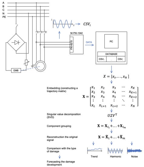
Figure 1.
General scheme of the study, including the SSA algorithm.
The experiment was performed in three machine states:
- Operation of the serviceable motor under standard conditions at rated load;
- Operation of the motor with one spall in the bearing inner ring at rated load;
- Operation of the motor with three spalls in the bearing inner ring at rated load.
For this experiment, a single-row, closed-type, deep-groove ball bearing 6208 ZZ C3 with shields was investigated (Figure 2, Table 2).
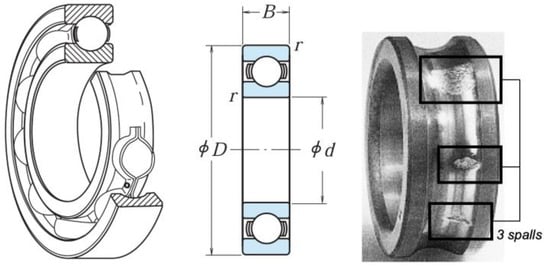
Figure 2.
Bearing 6208 ZZ C3.
Table 2.
Bearing data sheet.
It is possible to calculate the lifespan for each component of an induction motor, including bearings, but in practice a percentage of bearings breakdown before their lifespan. Throughout the bearing lifecycle, the main stages that have a significant impact on bearing life can be identified: bearing mounting and lubrication, alignment, relubrication, condition monitoring and dismounting. The most common causes of bearing damage are lubrication failures (36%), mounting failures (16%), lubricant contamination (14%) and fatigue wear (34%). Detecting a developing defect will significantly extend the bearing lifespan, thereby increasing the efficiency and productivity of the machinery in which the IM is used.
Three time series of motor current and voltage consumption were used as experimental data: the first set of data was without defects; two sets had 1 or 3 defects of the same type, respectively (spalls in the inner ring of the bearing), on the rear end shield. These time series had an identical sinusoidal structure; however, minor distortions were present, the nature of which was visually indeterminate (Figure 3).
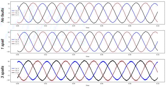
Figure 3.
Current signals for the bearing without faults, the bearing with one spall and the bearing with three spalls.
As is visible from the oscillograms, the presence of a defect with a single spall does not contribute to the current and voltage distortions. The further development of the defect appears as a current distortion, but this does not occur on the voltage. Therefore, in our case, the voltage signals are not of interest (Figure 4). However, in the case of a real process, the voltages may contain distortions that are determined by the presence of a non-linear and abruptly variable load on the common power bus [80]. In this case, the voltage time series should be used to find these distortions and to exclude their influence on the fault detection result, and subsequent studies can focus on this.
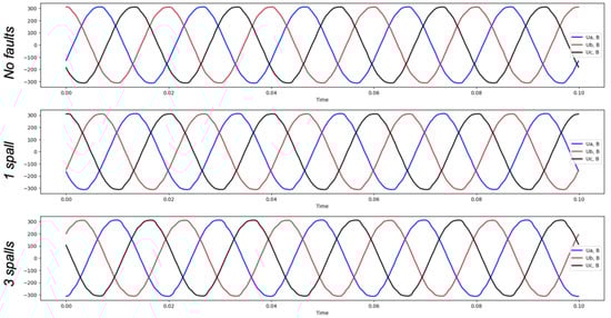
Figure 4.
Voltage signals for the bearing without faults, the bearing with one spall and the bearing with three spalls.
4. Performing Singular Spectrum Analysis
The core of the fault detection algorithm is the Singular Spectrum Analysis (SSA) method for processing the stator current signals. SSA is based on the decomposition of a time series into its elementary additive components, which allows its structure to be considered and investigated [81,82].
The SSA method consists of transforming a univariate series into a multivariate series using a single-parameter shift procedure, exploring the resulting multivariate trajectory using principal component analysis (singular decomposition) and reconstructing (approximating) the series using the selected principal components. The result of the method is a time series decomposed into simple components: trends, periodic or oscillatory components and noise components. The resulting decomposition components and their variations are compared with the operating mode and the level of the bearing fault. The identification of the necessary components can provide a basis for predicting both the time series itself and its individual components as the fault progresses and reaches the limit values. At the same time, the method does not require stationarity of the series, any knowledge of the trend, or knowledge of the presence of harmonic and cyclic components in the series.
The proposed algorithm, based on singular decomposition, can be applied for the detection of damage-related components, the smoothing of time series, for the investigation of changes during bearing degradation and for the evolution of bearing damages caused by wear.
4.1. Embedding (Constructing a Trajectory Matrix)
The IM phase current signals recorded in the file at a certain load mode and defect level were transformed into vector , representing an ordered set of instantaneous current values. Then, an embedding procedure was performed, representing the transformation of the original one-dimensional series of length into a sequence of -dimensional vectors, the number of which was equal to ; was the window length, :
These vectors formed a trajectory matrix of the original time series, which is Hankel’s and had the same elements on the diagonal :
4.2. Singular Value Decomposition
The singular decomposition for the matrix is a decomposition of the following form:
where is the unitary matrix of left singular vectors, is a unitary matrix of right singular vectors and is a diagonal matrix of size (Figure 5), whose diagonal elements are non-negative values of the singular values of the matrix in descending order, [72,83].
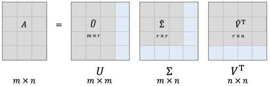
Figure 5.
Schematic representation of an SVD.
Matrix is also representable as a sum of submatrices:
where is the rank of the matrix ; respectively, is the submatrix of the i-th sub-signal.
To decompose the trajectory matrix obtained in the previous step, consider the matrix , with eigenvalues non-negative and in descending order. Let , be the corresponding eigenvectors of the matrix , and be the factorial vectors.
The decomposition of the trajectory matrix can then be written as follows:
where is the -th eigenvector of the singular decomposition containing the singular value , the left singular vector and the right singular vector of the trajectory matrix .
As a result of applying the SVD method, we obtain:
A visualization of the decomposed trajectory matrix into its components is necessary in order to assess the structure of the components in advance. An example of such a visualization for the A-phase signal is shown in Figure 6. A summary of the decomposition results for all phases is shown in Figure 7.
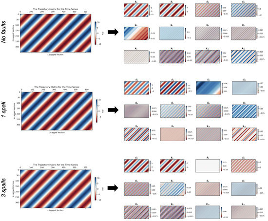
Figure 6.
Construction of trajectory matrices for phase A and their decomposition into 12 components for the bearing without faults, the bearing with one spall and the bearing with three spalls.
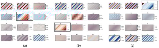
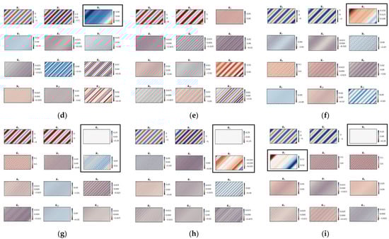
Figure 7.
Comparison of the trajectory matrix decomposition of all signals in consideration: bearing without faults (a–c); the bearing with one spall (d–f); the bearing with three spalls (g–i); phase A (a,d,g); phase B (b,e,h); phase C (c,f,i).
4.3. Component Grouping
This step is based on Equation (1). Let , then the resulting matrix , corresponding to group is defined as . The grouping procedure splits the whole set of indices into disjoint subsets . Then, the decomposition (Equation (5)) can be written in the form:
The procedure for sampling subsets represents the procedure for grouping own triples.
Several clustering approaches are considered in this study, and the clustering results are summarized in Table 4. The authors consider grouping results based on a visual assessment of the component matrix structure similarity, a method based on two-dimensional scatter plots and grouping based on the W-correlation matrix.
4.4. Reconstruction of the Original Signal
In the final step of the algorithm, each of the matrices of the decomposition (Equation (7)) is transformed back to the original form of the object . This operation is implemented using a Hankelization of matrices (diagonal averaging). The output is the closest matrix relative to the Frobenius norm, which respects the properties of the Hankel matrix and preserves its size.
Let , , . Usually , but for generality let , and . Let at , and otherwise. Let , and then the diagonal averaging equation for the matrix takes the form:
The diagonal averaging applied to each resulting component matrix creates a reconstructed time series. Thus, the original series is decomposed into the sum of the reconstructed series.
5. Results and Discussion
Based on the presented decomposition and grouping algorithm, the current signals of the three phases of the induction motor in the considered operating modes were processed.
Figure 7 shows the first 12 components of the original series in the form of Hankelized elementary matrices, arranged in descending order of their contribution to the reconstructed time series. There are no practical recommendations in the literature on the number of components to consider for damage analysis. The number of types of possible factors forming the current signal can be used to justify considering no more than 12 components out of the 350 singular values used in decomposing. The factors affecting the current signal, in addition to constructional motor and load features, also include the presence of defects. Consequently, the number of possible faults is a limit to be considered for significant components. The faults that can be detected by the electrical signals are bearing failure, shaft misalignment, inter-phase faults, eccentricity and rotor bar breakage.
Characteristic changes in several components, which are highlighted in the figure, are visually detectable. As the defect appears and increases, the non-stationary component increases its contribution to the overall signal structure, resulting in an increased order number. It should be noted that, in the presence of three spalls (that is, a clear appearance of the flaw) a degenerated component appears in all phases .
The estimation of the components’ relative contributions to the trajectory matrix, as well as the cumulative contribution, are calculated using the following equations:
The plots in Figure 8 show the relative and cumulative contributions of the first 12 components. Due to the significant contribution of the first two components, the plots are presented in pairs: the upper plots in each mode include all components, while the subsequent (lower) plots exclude the first two components for a better presentation.
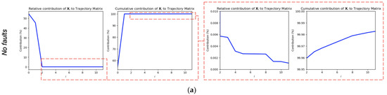
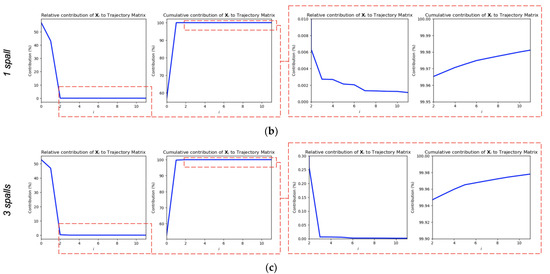
Figure 8.
Relative and cumulative contribution of the components: [0, …, 11] (left), [2, …, 11] (right) for phase A of the bearing without faults (a), the bearing with one spall (b) and the bearing with three spalls (c).
The complete result of the component contribution calculation is shown in Table 3.
Table 3.
Comparison of the results obtained from the component contribution calculations.
The estimation results show that the first 12 singular values describe 99.98% of the total information of the original signal in all three modes, and therefore a significant loss of informativeness is excluded. By highlighting the components that change on the diagnostic component map (Figure 7) when the spall occurs, we can compare the increase in contribution to the increase in defects. As can be seen from Table 3, the cumulative contribution of components and is more than 99%, making it impossible to track the manifestation of the defect at an early stage. There was no explicit correlation between changes in these components and the presence of the spall. In the presence of three spalls, the overall increase in the contribution of these components relative to the normal state was implicit. In order to unambiguously estimate the contribution and determine the manifestation of the component change in the current signal due to the presence of the initial stage of the defect, it was necessary to single out groups of lower-order components, which changed their position in the level of contribution in the presence of damage, and to estimate the change of their contribution in all three states.
Moreover, it is possible to determine the number of informative components based on the principal component similarity matrices calculated by the distance between pairs of Hankel matrices.
where is the Frobenius norm. Analyzing the distance matrix (Figure 9), we could distinguish a clear boundary in the range , which confirmed the similarity of the first components and discarded uninformative components .
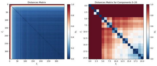
Figure 9.
Distance matrix based on the Frobenius norm for phase A of the bearing without faults, on the left for the complete set of components (350) and on the right for the investigated set of informative components (20).
The time series reconstruction from the component grouping results based on a visual assessment of the matrix structure is shown in Figure 10.
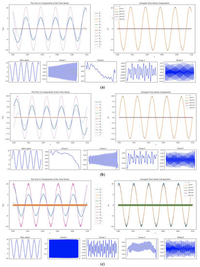
Figure 10.
Component grouping results based on visual assessment for phase A of the bearing without faults (a), the bearing with one spall (b) and the bearing with three spalls (c).
Due to the component’s poor visual separability, we propose considering two-dimensional scattergrams and grouping based on the W-correlation matrix to verify the component grouping hypotheses based on the visual comparison of the trajectory matrices.
Two-dimensional scattergrams are pairwise representations of the eigenvectors and for finding pairs of eigenvectors corresponding to the same harmonic. The orthogonality property of the eigenvectors allowed us to identify the harmonic as an image of a closed curve of regular shape (Figure 11).

Figure 11.
Scattergrams of eigenvectors for phase A of the bearing without faults, the bearing with one spall and the bearing with three spalls.
According to the figure, the smooth shape of the circle represents a distinct relationship between components 1 and 2 in each of the cases under consideration. Likewise, we can group components 5, 6, 7 and 8 together for a bearing without defects because of the similarly shaped closed curves. Additionally, for both cases of bearings with spalls, we could not combine component 2 with any of the neighboring groups.
The W-correlation matrix is used to verify and quantify the degree of separability between the elementary components. Correlation matrix analysis identifies pairs of correlated components and groups them together. Then, the measure of separability between the two reconstructed time series and is determined as follows:
where is the weighted internal (scalar) product, ; are the -th values of and , respectively; ; and for . The lower the value of , the higher the separability of the components; accordingly, if the reconstructed and were close to each other, then , and . , if and were orthogonal. This dependence (measure) is needed to calculate the dissimilarity when performing hierarchical clustering for automatic component grouping: .
The hierarchical clustering method consists of sequentially grouping similar pairs based on distances; the grouping continues until all objects form a single cluster. The result is a tree of groups, called a dendrogram, that represents the mutual relationships between objects in a given set (Figure 12). The number of groups depends on the threshold; the higher the threshold (Y-axis), the smaller the number of output groups.
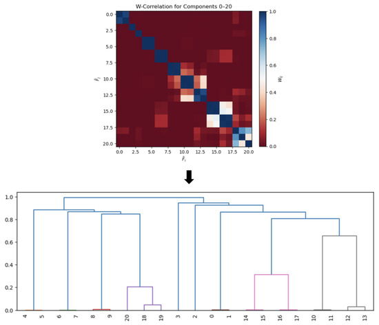
Figure 12.
Schematic diagram of the component grouping algorithm implementation.
Table 4 presents the results of the hierarchical clustering method and a comparison with scattergram-based grouping and visual grouping based on Hankel matrices. The combination of major components and occurred in all grouping methods regardless of the mode caused by the level of bearing defect. The second group varied depending on the method of grouping, phase numbering, and mode, but mainly component fell into this group; in variations where other components were added, there was always component . As the defect grew, we saw a steady increase in component and a decrease in component , and these trends were always opposite. As the damage increased in all phases, there was a regrouping, and component was grouped with component , equal in contribution, while component was singled out into a separate group with the largest contribution and degenerated. Each method of grouping was uniquely sensitive to the presence of a defect: in the presence of three spalls, grouping gave the same result regardless of the method. The presence of a defect resulted in a redistribution of the component composition and a change in the level of contribution. However, in the early stages of bearing degradation, the scattergram-based grouping method was more robust in isolating component into a separate group. Regardless of the grouping method, components and were the most important for tracking the manifestation of defects.
Table 4.
Comparison of the results obtained by grouping the components.
Indicators for tracking can be the structure of the components that compose the group and the total contribution they make to the overall signal. Future research is needed to analyze the grouping results in different ways to test the hypothesis of decomposition and mutual correlation in the presence of multiple combinations of defect levels and types. It is also of interest to reduce the data resolution to a level where the scattergram-based grouping method loses its ability to detect the initial and advanced stages of the defect.
6. Conclusions
The identification of faults in rotating equipment in general and induction motors in particular, based on the analysis of the electrical parameter, is a rather time-consuming yet relevant and promising task due to the complicated operating conditions of the equipment. The identification of vulnerabilities at an early stage of development in individual components will extend the lifecycle of the entire process and significantly reduce energy consumption and emissions.
In this paper, the authors proposed an approach based on the singular decomposition of the original sample applied to the electric motor stator current signal to identify the patterns characterizing the occurrence and evolution of the bearing fault. In order to verify the hypothesis of component extraction using SSA and SVD, experiments were performed and the results were explored using component contribution estimation; two-dimensional scatter plots and grouping by the hierarchical clustering method based on a weighted correlation matrix were considered for verification.
The results showed a tendency to isolate the components and into individual groups; this trend was evident in each of the given grouping approaches; also, the contribution of these grouped components increased by orders as the damage progressed steadily. The analysis of the obtained results allows the authors to conclude that these components are most likely to be responsible for fault development, thus confirming the possibility of identifying the defect at an early stage on the current signature basis by the proposed algorithm.
The proposed methodology has advantages over classical methods due to the lack of a need for additional sensors and the lack of additional knowledge of the original time series.
Research into other fault types, combinations of fault types and levels, and subsequent analysis of electrical signals using singular decomposition are of interest for future work by the authors.
In addition, future research includes:
- The investigation of the boundary sampling rate requirements for fault detection by the proposed algorithm;
- Testing the proposed algorithm on other non-obvious fault types, such as misalignment and loose motor mounts;
- The creation of a component map using the presented approaches for individual electromechanical equipment.
Identifying faults at an early stage and monitoring changes will allow for the intelligent management of maintenance and repair, as well as energy efficiency levels derived from the equipment’s technical condition.
Author Contributions
Conceptualization, Y.Z. and A.B.; methodology, Y.Z. and I.R.; software, A.B.; validation, I.R.; formal analysis, A.B.; investigation, A.B.; data curation, Y.Z.; writing—original draft preparation, A.B.; writing—review and editing, Y.Z. and I.R.; visualization, A.B.; supervision, Y.Z.; project administration, Y.Z. All authors have read and agreed to the published version of the manuscript.
Funding
The study was carried out at the expense of the subsidy for the state assignment in the field of scientific activity for 2023 “Fundamental interdisciplinary research of the Earth’s interior and processes of complex development of georesources” No. FSRW-2023-0002.
Data Availability Statement
The data presented in this study are available on request from the corresponding author.
Acknowledgments
The authors would like to acknowledge the Educational Research Center for Digital Technologies of the St Petersburg Mining University and Nikolay Korolev for providing the equipment, and Georgii Baranov from the ITMO University for providing support in data collection.
Conflicts of Interest
The authors declare no conflict of interest.
Abbreviation
| ANN | Artificial Neural Network |
| CO2 | Carbon Dioxide |
| DSS | Decision Support System |
| EEMD | Ensemble Empirical Mode Decomposition |
| EMB | Electromagnetic Brake |
| EMD | Empirical Mode Decomposition |
| FFT | Fast Fourier Transform |
| ICA | Independent Component Analysis |
| IM | Induction Motor |
| MRO | Maintenance and Repair |
| RPM | Revolutions Per Minute |
| SES | Square Envelope Spectrum |
| SSA | Singular Spectrum Analysis |
| STMS | Short-Term Matrix Series |
| SVD | Singular Value Decomposition |
| SVD-AF | Singular Value Decomposition Amplitude Filter |
| SVR | Singular Value Ration |
| VMD | Variation Mode Decomposition |
References
- Modarres, M.; Kaminskiy, M.; Krivtsov, V. Reliability Engineering and Risk Analysis: A Practical Guide; CRC: Boca Raton, FL, USA, 1999. [Google Scholar]
- Ustinov, D.A.; Shafhatov, E.R. Assessment of Reliability Indicators of Combined Systems of Offshore Wind Turbines and Wave Energy Converters. Energies 2022, 15, 9630. [Google Scholar] [CrossRef]
- Dodson, B.; Nolan, D. Reliability Engineering Handbook; CRC: Boca Raton, FL, USA, 1999. [Google Scholar]
- Brigton, S.; Long, Z.; Bunda, B. Evaluating and optimizing the effectiveness of mining equipment; the case of Chibuluma South underground mine. J. Clean. Prod. 2020, 252, 119697. [Google Scholar] [CrossRef]
- Malyshkov, G.B.; Sinkov, L.S.; Nikolaichuk, L.A. Analysis of economic evaluation methods of environmental damage at calculation of production efficiency in mining industry. Int. J. Appl. Eng. Res. 2017, 10, 2551–2554. [Google Scholar]
- Dvoynikov, M.; Sidorov, D.; Kambulov, E.; Rose, F.; Ahiyarov, R. Salt Deposits and Brine Blowout: Development of a Cross-Linking Composition for Blocking Formations and Methodology for Its Testing. Energies 2022, 15, 7415. [Google Scholar] [CrossRef]
- IEA. Energy Efficiency Policy Opportunities for Electric Motor-Driven Systems. 2011. Available online: https://www.iea.org/reports/energy-efficiency-policy-opportunities-for-electric-motor-driven-systems (accessed on 24 November 2022).
- IEA. Motor-Driven System Electricity Use as a Share of Electricity Use by Industry Subsector. 2020. Available online: https://www.iea.org/data-and-statistics/charts/motor-driven-system-electricity-use-as-a-share-of-electricity-use-by-industry-subsector (accessed on 24 November 2022).
- New EU Rules to Boost Energy Efficiency of Electric Motors. Available online: https://ec.europa.eu/info/news/new-eu-rules-boost-energy-efficiency-electric-motors-2021-jun-30_en (accessed on 24 November 2022).
- IEA. A Call to Action on Efficient and Smart Appliances. 2021. Available online: https://www.iea.org/articles/a-call-to-action-on-efficient-and-smart-appliances (accessed on 24 November 2022).
- Korolev, N.; Kozyaruk, A.; Morenov, V. Efficiency increase of energy systems in oil and gas industry by evaluation of electric drive lifecycle. Energies 2021, 14, 6074. [Google Scholar] [CrossRef]
- Khalturin, A.A.; Parfenchik, K.D.; Shpenst, V.A. Features of Oil Spills Monitoring on the Water Surface by the Russian Federation in the Arctic Region. J. Mar. Sci. Eng. 2023, 11, 111. [Google Scholar] [CrossRef]
- Tcvetkov, P. Engagement of resource-based economies in the fight against rising carbon emissions. Energy Rep. 2022, 8, 874–883. [Google Scholar] [CrossRef]
- Barabady, J.; Kumar, U. Reliability analysis of mining equipment: A case study of a crushing plant at Jajarm Bauxite Mine in Iran. Reliab. Eng. Syst. Saf. 2008, 93, 647–653. [Google Scholar] [CrossRef]
- Mitchell, Z. A Statistical Analysis of Construction Equipment Repair Costs Using Field Data and the Cumulative Cost Model; Virginia Polytechnic Institute: Blacksburg, VA, USA, 1998. [Google Scholar]
- Ercelebi, S.; Bascetin, A. Optimization of shovel-truck system for surface mining. J. S. Afr. Inst. Min. Metall. 2009, 109, 433–439. [Google Scholar]
- Salama, A.; Greberg, J. Optimization of truck-loader haulage system in an underground mine: A simulation approach using SimMine. In Proceedings of the 6th International Conference & Exhibition on Mass Mining, Sudbury, ON, Canada, 10–14 June 2012. [Google Scholar]
- Khandelwal, M.; Singh, T. Prediction of blast-induced ground vibration using artificial neural network. Int. J. Rock Mech. Min. Sci. 2009, 46, 1214–1222. [Google Scholar] [CrossRef]
- Khandelwal, M.; Kumar, D.; Yellishetty, M. Application of soft computing to predict blast-induced ground vibration. Eng. Comput. 2011, 27, 117–125. [Google Scholar] [CrossRef]
- Zhongya, Z.; Xiaoguang, J. Prediction of peak velocity of blasting vibration based on artificial neural network optimized by dimensionality reduction of FA-MIV. Math. Probl. Eng. 2018, 2018, 8473547. [Google Scholar] [CrossRef]
- Lavrenko, S.A.; Shishljannikov, D.I. Performance evaluation of heading-and-winning machines in the conditions of potash mines. Appl. Sci. 2021, 11, 3444. [Google Scholar] [CrossRef]
- Desai, C.; Shaikh, A. Drill wear monitoring using artificial neural network with differential evolution learning. In Proceedings of the 2006 IEEE International Conference Industry Technology, IEEE, Mumbai, India, 15–17 December 2006; pp. 2019–2022. [Google Scholar] [CrossRef]
- Lashari, S.; Takbiri-Borujeni, A.; Fathi, E.; Sun, T.; Rahmani, R.; Khazaeli, M. Drilling performance monitoring and optimization: A data-driven approach. J. Pet. Explor. Prod. Technol. 2019, 9, 2747–2756. [Google Scholar] [CrossRef]
- Zemenkova, M.Y.; Chizhevskaya, E.L.; Zemenkov, Y.D. Intelligent monitoring of the condition of hydrocarbon pipeline transport facilities using neural network technologies. J. Min. Inst. 2022, 258, 933–944. [Google Scholar] [CrossRef]
- Filippov, E.V.; Zakharov, L.A.; Martyushev, D.A.; Ponomareva, I.N. Reproduction of reservoir pressure by machine learning methods and study of its influence on the cracks formation process in hydraulic fracturing. J. Min. Inst. 2022, 258, 924–932. [Google Scholar] [CrossRef]
- Klyuev, R.; Fomenko, O.; Gavrina, O.; Turluev, R.; Marzoev, S. Energy indicators of drilling machines and excavators in mountain territories. Adv. Intell. Syst. Comput. (EMMFT 2019) 2021, 1258, 272–281. [Google Scholar] [CrossRef]
- Sychev, Y.A.; Zimin, R.Y. Improving the quality of electricity in the power supply systems of the mineral resource complex with hybrid filter-compensating devices. J. Min. Inst. 2021, 247, 132–140. [Google Scholar] [CrossRef]
- Shaobo, X.; Xiaosong, H.; Shanwei, Q.; Xiaolin, T.; Kun, L.; Zongke, X.; Brighton, J. Model predictive energy management for plug-in hybrid electric vehicles considering optimal battery depth of discharge. Energy 2019, 173, 667–678. [Google Scholar] [CrossRef]
- Shuo, Z.; Xiaosong, H.; Shaobo, X.; Ziyou, S.; Lin, H.; Cong, H. Adaptively coordinated optimization of battery ageing and energy management in plug-in hybrid electric buses. Appl. Energy 2019, 256, 113891. [Google Scholar] [CrossRef]
- Xuebing, H.; Languang, L.; Yuejiu, Z.; Xuning, F.; Zhe, L.; Jianqiu, L.; Minggao, O. A review on the key issues of the lithium-ion battery degradation among the whole life cycle. ETransportation 2019, 1, 100005. [Google Scholar] [CrossRef]
- Yanbiao, F.; Zuomin, D. Optimal energy management with balanced fuel economy and battery life for large hybrid electric mining truck. J. Power Sources 2020, 454, 227948. [Google Scholar] [CrossRef]
- Sychev, Y.A.; Kostin, V.N.; Serikov, V.A.; Aladin, M.E. Nonsinusoidal modes in power-supply systems with nonlinear loads and capacitors in mining. Min. Inf. Anal. Bull. (MIAB) 2023, 1, 159–179. [Google Scholar] [CrossRef]
- Nikolaev, A.V.; Vöth, S.; Kychkin, A.V. Application of the cybernetic approach to price-dependent demand response for underground mining enterprise electricity consumption. J. Min. Inst. 2022, 256, 686. [Google Scholar] [CrossRef]
- Klyuev, R.V.; Morgoev, I.D.; Morgoeva, A.D.; Gavrina, O.A.; Martyushev, N.V.; Efremenkov, E.A.; Mengxu, Q. Methods of Forecasting Electric Energy Consumption: A Literature Review. Energies 2022, 15, 8919. [Google Scholar] [CrossRef]
- Gundewar, S.K.; Kane, P.V. Condition Monitoring and Fault Diagnosis of Induction Motor. J. Vib. Eng. Technol. 2021, 9, 643–674. [Google Scholar] [CrossRef]
- Zhao, Z.; Li, T.; Wu, J.; Sun, C.; Wang, S.; Yan, R.; Chen, X. Deep learning algorithms for rotating machinery intelligent diagnosis: An open source benchmark study. ISA Trans. 2020, 107, 224–255. [Google Scholar] [CrossRef]
- Gangsar, P.; Tiwari, R. Signal based condition monitoring techniques for fault detection and diagnosis of induction motors: A state-of-the-art review. Mech. Syst. Signal Process. 2020, 144, 106908. [Google Scholar] [CrossRef]
- Soomro, A.A.; Mokhtar, A.A.; Kurnia, J.C.; Lashari, N.; Lu, H.; Sambo, C. Integrity assessment of corroded oil and gas pipelines using machine learning: A systematic review. Eng. Fail. Anal. 2022, 131, 105810. [Google Scholar] [CrossRef]
- Cui, Y.; Kara, S.; Chan, K.C. Manufacturing big data ecosystem: A systematic literature review. Robot. Comput.-Integr. Manuf. 2020, 62, 101861. [Google Scholar] [CrossRef]
- Kahr, M.; Kovács, G.; Loinig, M.; Brückl, H. Condition Monitoring of Ball Bearings Based on Machine Learning with Synthetically Generated Data. Sensors 2022, 22, 2490. [Google Scholar] [CrossRef]
- Chelmiah, E.T.; McLoone, V.I.; Kavanagh, D.F. Remaining Useful Life Estimation of Rotating Machines through Supervised Learning with Non-Linear Approaches. Appl. Sci. 2022, 12, 4136. [Google Scholar] [CrossRef]
- Bejaoui, I.; Bruneo, D.; Xibilia, M.G. Remaining Useful Life Prediction of Broken Rotor Bar Based on Data-Driven and Degradation Model. Appl. Sci. 2021, 11, 7175. [Google Scholar] [CrossRef]
- Ferreira, C.; Gonçalves, G. Remaining Useful Life prediction and challenges: A literature review on the use of Machine Learning Methods. J. Manuf. Syst. 2022, 63, 550–562. [Google Scholar] [CrossRef]
- Lv, H.; Chen, J.; Pan, T.; Zhang, T.; Feng, Y.; Liu, S. Attention mechanism in intelligent fault diagnosis of machinery: A review of technique and application. Measurement 2022, 199, 111594. [Google Scholar] [CrossRef]
- Kudelina, K.; Vaimann, T.; Rassõlkin, A.; Kallaste, A.; Demidova, G.; Karpovich, D. Diagnostic Possibilities of Induction Motor Bearing Currents. In Proceedings of the 2021 XVIII International Scientific Technical Conference Alternating Current Electric Drives (ACED), Ekaterinburg, Russia, 24–27 May 2021; pp. 1–5. [Google Scholar] [CrossRef]
- Merizalde, Y.; Hernández-Callejo, L.; Duque-Perez, O. State of the Art and Trends in the Monitoring, Detection and Diagnosis of Failures in Electric Induction Motors. Energies 2017, 10, 1056. [Google Scholar] [CrossRef]
- Grasso, M.; Chatterton, S.; Pennacchi, P.; Colosimo, B.M. A data-driven method to enhance vibration signal decomposition for rolling bearing fault analysis. Mech. Syst. Signal Process. 2016, 81, 126–147. [Google Scholar] [CrossRef]
- Zhou, X.; Mao, S.; Li, M. A Novel Anti-Noise Fault Diagnosis Approach for Rolling Bearings Based on Convolutional Neural Network Fusing Frequency Domain Feature Matching Algorithm. Sensors 2021, 21, 5532. [Google Scholar] [CrossRef]
- Yakhni, M.F.; Cauet, S.; Sakout, A.; Assoum, H.; Etien, E.; Rambault, L.; El-Gohary, M. Variable speed induction motors’ fault detection based on transient motor current signatures analysis: A review. Mech. Syst. Signal Process. 2023, 184, 109737. [Google Scholar] [CrossRef]
- Wu, G.; Yan, T.; Yang, G.; Chai, H.; Cao, C. A Review on Rolling Bearing Fault Signal Detection Methods Based on Different Sensors. Sensors 2022, 22, 8330. [Google Scholar] [CrossRef]
- Wang, L.; Liu, Z.; Liu, A.; Tao, F. Artificial intelligence in product lifecycle management. Int. J. Adv. Manuf. Technol. 2021, 114, 771–796. [Google Scholar] [CrossRef]
- Kumar, N.M.; Chand, A.A.; Malvoni, M.; Prasad, K.A.; Mamun, K.A.; Islam, F.R.; Chopra, S.S. Distributed Energy Resources and the Application of AI, IoT, and Blockchain in Smart Grids. Energies 2020, 13, 5739. [Google Scholar] [CrossRef]
- Koteleva, N.; Loseva, E. Development of an Algorithm for Determining Defects in Cast-in-Place Piles Based on the Data Analysis of Low Strain Integrity Testing. Appl. Sci. 2022, 12, 10636. [Google Scholar] [CrossRef]
- Beloglazov, I.I.; Sabinin, D.S.; Nikolaev, M.Y. Modeling the disintegration process for ball mills using dem. MIAB. Min. Inf. Anal. Bull. 2022, 6, 268–282. [Google Scholar] [CrossRef]
- Baranov, G.; Nepomuceno, E.; Vaganov, M.; Ostrovskii, V.; Butusov, D. New Spectral Markers for Broken Bars Diagnostics in Induction Motors. Machines 2020, 8, 6. [Google Scholar] [CrossRef]
- Raja, H.; Kudelina, K.; Asad, B.; Vaimann, T.; Kallaste, A.; Rassõlkin, A.; Khang, H.V. Signal Spectrum-Based Machine Learning Approach for Fault Prediction and Maintenance of Electrical Machines. Energies 2022, 15, 9507. [Google Scholar] [CrossRef]
- AlShalalfeh, A.; Shalalfeh, L. Bearing Fault Diagnosis Approach under Data Quality Issues. Appl. Sci. 2021, 11, 3289. [Google Scholar] [CrossRef]
- Wang, Y.; Xiao, Z.; Cao, G. A convolutional neural network method based on Adam optimizer with power-exponential learning rate for bearing fault diagnosis. J. Vibroeng. 2022, 24, 666–678. [Google Scholar] [CrossRef]
- Ciszewski, T.; Gelman, L.; Ball, A. Novel Nonlinear High Order Technologies for Damage Diagnosis of Complex Assets. Electronics 2022, 11, 3885. [Google Scholar] [CrossRef]
- Shabalov, M.Y.; Zhukovskiy, Y.L.; Buldysko, A.D.; Gil, B.; Starshaia, V.V. The influence of technological changes in energy efficiency on the infrastructure deterioration in the energy sector. Energy Rep. 2021, 7, 2664–2680. [Google Scholar] [CrossRef]
- Xu, M.; Marangoni, R.D. Vibration analysis of a motor-flexible coupling-rotor system subject to misalignment and unbalance, Part I: Theoretical model and analysis. J. Sound Vib. 1994, 176, 663–679. [Google Scholar] [CrossRef]
- Abouelanouar, B.; Elkihel, A.; Gziri, H. Experimental study on energy consumption in rotating machinery caused by misalignment. SN Appl. Sci. 2020, 2, 1215. [Google Scholar] [CrossRef]
- Choudhary, A.; Goyal, D.; Shimi, S.L.; Akula, A. Condition Monitoring and Fault Diagnosis of Induction Motors: A Review. Arch. Computat. Methods Eng. 2019, 26, 1221–1238. [Google Scholar] [CrossRef]
- Khan, M.A.; Asad, B.; Kudelina, K.; Vaimann, T.; Kallaste, A. The Bearing Faults Detection Methods for Electrical Machines—The State of the Art. Energies 2023, 16, 296. [Google Scholar] [CrossRef]
- Ambrozkiewicz, B.; Litak, G.; Georgiadis, A.; Syta, A.; Meier, N.; Gassner, A. Effect of Radial Clearance on Ball Bearing’s Dynamics Using a 2-DOF Model. Int. J. Simul. Model 2021, 20, 513–524. [Google Scholar] [CrossRef]
- Russell, T.; Sadeghi, F.; Peterson, W.; Aamer, S.; Arya, U. A Novel Test Rig for the Investigation of Ball Bearing Cage Friction. Tribol. Trans. 2021, 64, 943–955. [Google Scholar] [CrossRef]
- Xu, L.; Chatterton, S.; Pennacchi, P. Rolling element bearing diagnosis based on singular value decomposition and composite squared envelope spectrum. Mech. Syst. Signal Process. 2021, 148, 107174. [Google Scholar] [CrossRef]
- Golyandina, N.; Korobeynikov, A. Basic Singular Spectrum Analysis and forecasting with R. Comput. Stat. Data Anal. 2014, 71, 934–954. [Google Scholar] [CrossRef]
- Doynikov, A.N.; Salnikova, M.K.; Kalinin, M.P. Method for predicting non-stationary processes in structurally unstable systems. Mod. Technol. Syst. Analysis. Model. 2008, 2, 119–123. (In Russian) [Google Scholar]
- Golyandina, N.E. Particularities and commonalities of singular spectrum analysis as a method of time series analysis and signal processing. WIREs Comput. Stat. 2020, 12, e1487. [Google Scholar] [CrossRef]
- Zhao, X.; Ye, B. Feature frequency extraction algorithm based on the singular value decomposition with changed matrix size and its application in fault diagnosis. J. Sound Vib. 2022, 526, 116848. [Google Scholar] [CrossRef]
- Guo, M.; Li, W.; Yang, Q.; Zhao, X.; Tang, Y. Amplitude filtering characteristics of singular value decomposition and its application to fault diagnosis of rotating machinery. Measurement 2020, 154, 107444. [Google Scholar] [CrossRef]
- Zhao, X.; Ye, B. Similarity of signal processing effect between Hankel matrix-based SVD and wavelet transform and its mechanism analysis. Mech. Syst. Signal Process. 2009, 23, 1062–1075. [Google Scholar] [CrossRef]
- Azouzi, K.; Boudinar, A.H.; Aimer, F.A.; Bendiabdellah, A. Use of a combined SVD-Kalman filter approach for induction motor broken rotor bars identification. J. Microw. Optoelectron. Electromagn. Appl. 2018, 17, 85–101. [Google Scholar] [CrossRef]
- Cong, F.; Chen, J.; Dong, G.; Zhao, F. Short-time matrix series based singular value decomposition for rolling bearing fault diagnosis. Mech. Syst. Signal Process. 2013, 34, 218–230. [Google Scholar] [CrossRef]
- Zhao, H.; Sun, M.; Deng, W.; Yang, X. A New Feature Extraction Method Based on EEMD and Multi-Scale Fuzzy Entropy for Motor Bearing. Entropy 2017, 19, 14. [Google Scholar] [CrossRef]
- Isham, M.F.; Leong, M.S.; Lim, M.H.; Ahmad, Z.A. Variational Mode Decomposition: Mode Determination Method for Rotating Machinery Diagnosis. J. Vibroeng. 2018, 20, 2604–2621. [Google Scholar] [CrossRef]
- Wang, H.; Li, R.; Tang, G.; Yuan, H.; Zhao, Q.; Cao, X. A Compound Fault Diagnosis for Rolling Bearings Method Based on Blind Source Separation and Ensemble Empirical Mode Decomposition. PLoS ONE 2014, 9, e109166. [Google Scholar] [CrossRef]
- SKF. Damage to Rolling Bearings and Their Cause. (In Russian). Available online: https://www.promshop.info/cataloguespdf/reasons_damage_bearings.pdf (accessed on 24 November 2022).
- Skamyin, A.; Shklyarskiy, Y.; Dobush, I.; Dobush, V.; Sutikno, T.; Jopri, M.H. An assessment of the share contributions of distortion sources for various load parameters. International. J. Power Electron. Drive Syst. (IJPEDS) 2022, 13, 950. [Google Scholar] [CrossRef]
- Kuzmin, O.V.; Kedrin, V.S. Analysis of the structure of harmonic series of dynamics based on the singular value decomposition algorithm. Manag. Probl. 2013, 1, 26–31. (In Russian) [Google Scholar]
- Revin, I.; Potemkin, V.A.; Balabanov, N.R.; Nikitin, N.O. Automated machine learning approach for time series classification pipelines using evolutionary optimization. Knowl.-Based Syst. 2023, 268, 110483. [Google Scholar] [CrossRef]
- Xu, L.; Chatterton, S.; Pennacchi, P.; Liu, C. A Tacholess Order Tracking Method Based on Inverse Short Time Fourier Transform and Singular Value Decomposition for Bearing Fault Diagnosis. Sensors 2020, 20, 6924. [Google Scholar] [CrossRef] [PubMed]
Disclaimer/Publisher’s Note: The statements, opinions and data contained in all publications are solely those of the individual author(s) and contributor(s) and not of MDPI and/or the editor(s). MDPI and/or the editor(s) disclaim responsibility for any injury to people or property resulting from any ideas, methods, instructions or products referred to in the content. |
© 2023 by the authors. Licensee MDPI, Basel, Switzerland. This article is an open access article distributed under the terms and conditions of the Creative Commons Attribution (CC BY) license (https://creativecommons.org/licenses/by/4.0/).