Extended Operating Region Algorithm for PV Array Connected to Microgrids for Wide Frequency and Amplitude Variations

Abstract

The employment of microgrids and distributed power generation have exponentially increased over recent decades, due in part to the increased inclusion of renewable energies as these technologies become cheaper to install. However, microgrids are highly sensitive to power variation, leading to distortion of the grid voltage (amplitude and frequency changes) which could destabilize the entire microgrid under variation of loads and/or other power sources. In this context, a new control strategy is proposed for a photovoltaic grid connected system, operating under voltage variations typical of a low inertial electric power network. The main problem related to voltage fluctuation is that the variables may take the power converter out of the operating region, and therefore, all controllers, including the maximum power point tracking, will not work as designed. The analysis, based on the mathematical operating region, demonstrates that the control strategy can include overmodulation compensation—to overcome problems related to weak microgrids and systems variations—through the addition of smart power factor imposition and DC-link voltage variation in transient time when the variables are far from the nominal values. The proposal is validated through simulation in PSim^®/Matlab^® and implementation on a laboratory prototype, showing the feasibility of the designed algorithm.

1. Introduction

Renewable energies have become a replacement for conventional means of electrical power generation [1,2,3]. Specifically, photovoltaic systems are of particular interest and therefore have been widely studied [1]. The incorporation of renewable energy sources (RES) has helped to distribute clean energy and increase the proliferation of microgrids with everlasting power when compared with traditional fuel ones [4].

Due to the low inertia of microgrids, they are greatly affected by power unbalancing between generation and consumption, leading to amplitude and frequency fluctuations [5,6]. Frequency variations—up to 100%—have been reported in applications such as aircraft, electrical ships, ferries, vessels, and seaports, among others [2,4]. This is the reason power converters need to employ algorithms capable of addressing these conditions and, subsequently, be able to integrate with systems such as those aforementioned.

To inject power energy into the AC grid, two approaches can be employed: (i) include a transition DC–DC converter and then a DC–AC inverter or (ii) only include a DC–AC stage, which reduces losses since one stage is removed [7]. In other words, maximum power extraction and injection can be carried out with a direct DC/AC converter topology [8,9]. Therefore, the DC-link voltage is managed directly by the maximum power point tracking (MPPT) algorithm, e.g., a P&O algorithm [8,10,11,12]. This means a simplification in the topology used for power conversion since fewer elements and less physical space is used [13].

In addition to the maximum power point tracking, power injection into the grid also requires synchronization algorithms, such as Phase-Locked Loop (PLL), to accurately track the grid frequency and phase shifting, as shown in references [14,15,16,17]. In this paper, the proposed control strategy employs a PLL algorithm, similar to that presented in [14], in order to allow the converter to operate effectively under a wide range of frequencies, such as the conditions of microgrids herein employed.

Frequency and amplitude variations are part of the operation of microgrids and weak-grid systems [14]; therefore, power converters connected to these kinds of networks require controllers capable of avoiding a fall into overmodulation or even instability [4]. Research conducted in [18] has demonstrated that variations in microgrid voltage can result in variations in the operating region. Specifically, when the frequency increases, the operating region is reduced due to an increase in passive filter impedance. On the other hand, under voltage swell conditions, the operating region is also decreased due to a reduction in the voltage difference between the injected voltage (v_o^abc, due to the DC voltage) and the grid voltage v_s^abc, as described in [19,20]. It is crucial to note that power converters connected to microgrids may fall out of the operating region, and as such, power converter control must be designed to work under these conditions.

Due to the converter operating region studied, some of the latest control strategies propose a limit control on the Active/Reactive Power (PQ) plane operating region under unfavorable conditions [20,21]. These papers propose a way to overcome this issue by modifying the operating region in order to avoid overmodulation, which is the result of working out of the operating region.

As previously mentioned, the operating region can be reduced due to the operating conditions of a microgrid; for example, an increase in voltage frequency and/or swell amplitude variation. Therefore, in this work, a control method to overcome the operating region issue is presented; specifically, overmodulation is overcome by including the modification of the power factor and increasing the DC-link voltage whilst trying to maintain solar energy injection as high as possible. The proposed algorithm is designed for a single-stage DC/AC converter, and thus, increasing the DC voltage requires stepping away from the maximum power point (MPP) and should therefore be avoided as much as possible and only employed when necessary to overcome overmodulation, which may lead to instability. As a result, an overmodulation protection algorithm is proposed that allows the converter to continue operating over a wide frequency range and sag/swell conditions, at the cost of briefly losing the MPP of the photovoltaic system and the unit power factor.

The proposed control strategy is simulated and applied to a photovoltaic system using PSim© software. Finally, several experimental tests are carried out to validate the model by means of a laboratory prototype setup and the use of a TMS320F28335 digital signal controller (DSC) board from Texas Instruments to visualize some of the internal control variables through the graphics tool of the Code Composer Studio software. The most relevant conclusions of the work are also included.

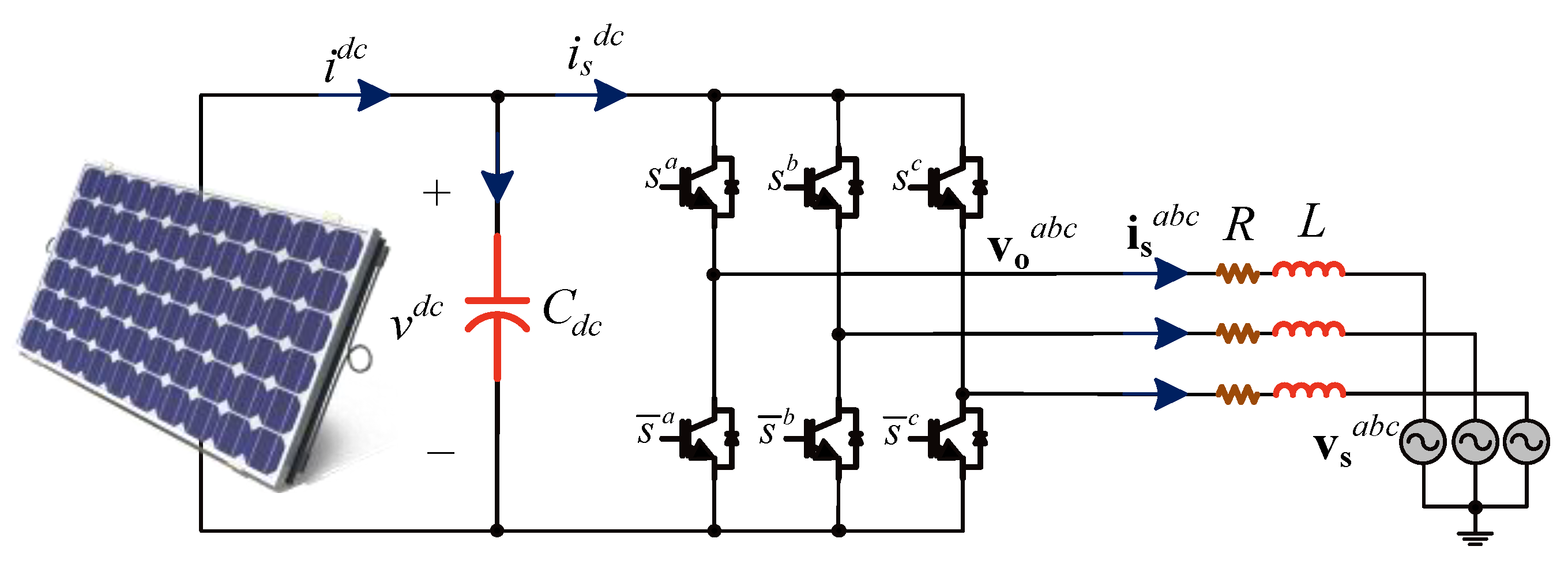
2. Power Converter Model

A PV system connected to the point of common coupling (PCC) using a Voltage Source Inverter (VSI) configuration is shown in Figure 1. It can be mathematically modeled through the Kirchhoff laws.

Employing the SPWM modulation technique, with injected voltage v_o^abc and injected current i_s^dc, can be defined as:

$$v_o{}^{abc}=G_{ac}{m}^{abc}{v}^{dc}\mathrm{and}{i}_s{}^{dc}=G_{ac}{(m^{abc})}^T{i}_s{}^{abc}$$

(1)

where G_ac represents the modulation technique gain and m^abc, the modulation function for each phase.

Analyzing the circuit in Figure 1, the voltage equation on the AC side results in:

$$v_o{}^{abc}=R{i}_s{}^{abc}+L\frac{d{i}_s{}^{abc}}{dt}+v_s{}^{abc}\Rightarrow \frac{d{i}_s{}^{abc}}{dt}=\frac{G_{ac}{v}^{dc}}{L}{m}^{abc}-\frac{R}{L}{i}_s{}^{abc}-\frac{1}{L}{v}_s{}^{abc}$$

(2)

On the other hand, on the DC side, it can be found that i^dc = i_c + i_s^dc, and therefore the DC-link capacitor model including (1) results in:

$$C_{dc}\frac{d{v}^{dc}}{dt}=i^{dc}-i_s{}^{dc}\Rightarrow \frac{d{v}^{dc}}{dt}=\frac{1}{C_{dc}}\left(i^{dc}-G_{ac}{(m^{abc})}^T{i}_s{}^{abc}\right)$$

(3)

Thus, Equations (2) and (3) model the power system dynamically. However, to work with continuous variables, the dq Park Transformation can be employed. Then, over the continuous variables system, it is possible to apply classical control theory to manage the currents and voltages. Consequently, by applying the Park transform to Equations (2) and (3), it is obtained:

$$\frac{d{i}_s{}^{dq}}{dt}=\frac{1}{L}{G}_{ac}{m}^{dq}{v}^{dc}-\frac{R}{L}{i}_s{}^{dq}-W{i}_s{}^{qd}-\frac{1}{L}{v}_s{}^{dq}$$

(4)

where W = $\left[\begin{array}{cc}0& -\omega \\ \omega & 0\end{array}\right]$, ω = 2πf, and f is the grid frequency.

$$\frac{d{v}^{dc}}{dt}=\frac{1}{C_{dc}}\left(i^{dc}-G_{ac}\left(i_s{}^d{m}^d+i_s{}^q{m}^q\right)\right)$$

(5)

Therefore, the nonlinear dynamic model of the system in Figure 1 is depicted in Equations (4) and (5).

3. Operation Region

In most grid-tied applications, the voltage maintains constant parameters (frequency and amplitude) and, consequently, the control is designed under these circumstances. However, in microgrids, the voltage frequency and amplitude may vary considerably due to their small electric system inertia [22]. These variations affect the converters and their respective operating regions [23].

A study of the operating region allows us to obtain the set of operation points where no overmodulation is reached. In addition, it helps to mark off the zone where the power converter engages overmodulation and, therefore, the model in (4) and (5) is not valid. Such a region is computed when the converter is in steady state, i.e., the derivations in (4) and (5) are equal to zero because the model is in dq reference frame. Thus, the operating region is found from the following equations:

$$0=\frac{1}{L}{G}_{ac}{m}^{dq}{v}^{dc}-\frac{R}{L}{i}_s{}^{dq}-W{i}_s{}^{qd}-\frac{1}{L}{v}_s{}^{dq}$$

(6)

$$0=\frac{1}{C}\left(i^{dc}-G_{ac}\left(i_s{}^d{m}^d+i_s{}^q{m}^q\right)\right)$$

(7)

In addition, the equation that relates the power factor (pf) and the currents in the synchronous axis can be stated as:

$$i_s{}^q=-i_s{}^d\tan \left({\cos }^{-1}\left(pf\right)\right)$$

(8)

Subsequently, it is possible determine a relationship for m^dq, as a function of the state variables and system parameters, as:

$$m^d=\frac{pf\cdot v_s{}^d+R\cdot pf\cdot i_s{}^d+L\cdot i_s{}^d\cdot \omega \sqrt{\left(1-p{f}^2\right)}}{G_{ac}\cdot pf\cdot v^{dc}}$$

(9)

$$m^q=\frac{pf\cdot v_s{}^q-R\cdot i_s{}^d\sqrt{\left(1-p{f}^2\right)}+L\cdot pf\cdot i_s{}^d\mathsf{\omega }}{G_{ac}\cdot pf\cdot v^{dc}}$$

(10)

where the q-axis current is:

$$i_s{}^q=-i_s{}^d\frac{\sqrt{1-p{f}^2}}{pf}$$

(11)

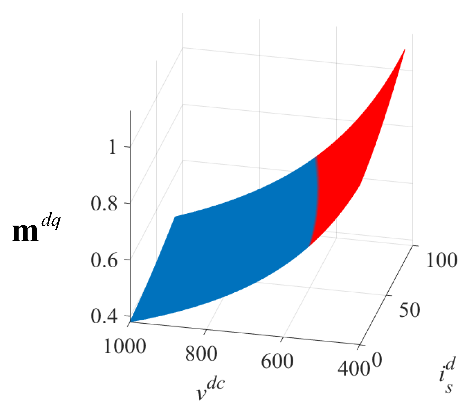
Then, to obtain the operating region, a sweep for values of v^dc and i^dq is performed. These values are entered into a Matlab^® script and all possible values of modulators are obtained, delivering the overmodulation information. One way to see the region graphically is by considering a valid model (VM) and a not valid model (NVM), which represent no overmodulation and with overmodulation, respectively. Therefore, to avoid this issue, and considering a carrier from −0.5 to 0.5 p.u., the modulator amplitude condition that must be met is the following:

$$M_{dq}=\sqrt{\left(\raisebox{1ex}{$2$}\!\left/ \!\raisebox{-1ex}{$3$}\right.\right)}\sqrt{{\left(m^d\right)}^2+{\left(m^q\right)}^2}\le 0.5$$

(12)

To graph the operating region considering the restriction in (12), the parameters of the system must be defined, which are listed in

Table 1. Inverter simulation parameters.

Parameter	Value
Vs	380 Vrms
R	0.4 Ω
L	7 mH
Cdc	2.35 mF
vdc	660–900 V
isd	0–85 A
pf	Unitary
f	50 Hz

.

The simulation is performed in Matlab^® to obtain the 3D plot of the operating region, presented in Figure 2. The plot shows the overmodulation zone in red, and in blue when Equation (12) is satisfied, i.e., where the model is valid.

Other interesting cases to analyze involve how the operating region behaves under different power factors. The main studied cases are: (i) unity, (ii) inductive pf of 0.93, and (iii) capacitive pf of 0.93. The simulation results of the three cases are presented in Figure 3, operating with a fixed frequency of 50 Hz. It can be observed that the converter has the greatest valid model (VM) region when the pf is inductive, a smaller region for unity pf, and the smallest VM region when capacitive pf is imposed.

The effect of changing the pf on the power converter operating region is summarized in

Table 2. Variation of operation region due to variation of pf_ref.

Parameter	Value	%Variation
pfref	1	0% (reference)
pfref	0.93 (inductive)	12.5708%
pfref	0.93 (capacitive)	−12.2076%

, where the unity pf is taken as the reference. It is easy to note that the operating region is increased by around 12% for an inductive pf and reduced by around 12% for a capacitive pf. This result presents an opportunity to increase the operating region.

It is important to highlight that frequency affects the operating region because of the natural frequency response of inductances and capacitances. Figure 4 shows the results considering a unitary pf, tested for different frequencies: 30 Hz, 50 Hz, and 100 Hz. It can be observed that the greater the frequency value, the smaller the valid model operating region obtained. Therefore, with a lower frequency and more inductive pf, a greater linear operation region can be obtained for the inverter. However, in this case, frequency is a disturbance and cannot be employed to enlarge the operating region, but the control can be aware that increasing frequency will decrease the operating region.

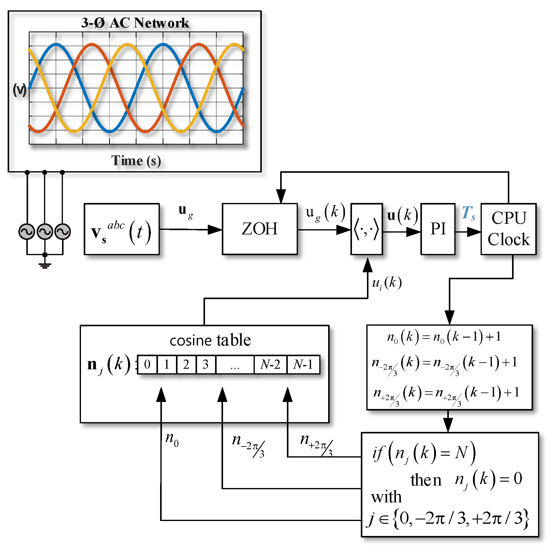
4. Phase-Locked-Loop

To ensure proper current control, the power converter needs to be synchronized with the grid mains, and the Phase Lock Loops (PLL) algorithm is one of the solutions to achieve phase tracking [14].

The synchronizer used in this work seeks to maintain N samples per period independent of the grid frequency (external signal), i.e., the algorithm constantly changes the sampling time to track the grid frequency.

This PLL operates based on two variables: an external variable, u_g, and an internal variable. The external variable is sensed from the three-phase voltage and can be mathematically represented as:

$$u_g=U_g{\left[\begin{array}{ccc}\sin \left({\theta }_g\right)& \sin \left({\theta }_g-\frac{2\pi }{3}\right)& \sin \left({\theta }_g+\frac{2\pi }{3}\right)\end{array}\right]}^T$$

(13)

Similarly, the internal variable has a behavior that can be described as:

$$u_i(k)={\left[\begin{array}{ccc}\mathrm{cosine}\left(n_0\left(k\right)\right)& \mathrm{cosine}\left(n_{\raisebox{1ex}{$-2\pi $}\!\left/ \!\raisebox{-1ex}{$3$}\right.}\left(k\right)\right)& \mathrm{cosine}\left(n_{\raisebox{1ex}{$+2\pi $}\!\left/ \!\raisebox{-1ex}{$3$}\right.}\left(k\right)\right)\end{array}\right]}^T$$

(14)

where cosine(∙) represents the N samples discretization of the cosine function, such that:

$$\mathrm{cosine}\left(m\right)=\cos \left(\frac{2\pi }{3}m\right),m\in \left\{0,1,2,\dots ,N-1\right\}$$

(15)

Each sampling time updates the values of $n_0\left(k\right)$, $n_{\raisebox{1ex}{$-2\pi $}\!\left/ \!\raisebox{-1ex}{$3$}\right.}\left(k\right)$, and $n_{\raisebox{1ex}{$+2\pi $}\!\left/ \!\raisebox{-1ex}{$3$}\right.}\left(k\right)$ according to:

$$n_0\left(k\right)=n_0\left(k-1\right)+1$$

(16)

$$n_{\raisebox{1ex}{$-2\pi $}\!\left/ \!\raisebox{-1ex}{$3$}\right.}\left(k\right)=n_{\raisebox{1ex}{$-2\pi $}\!\left/ \!\raisebox{-1ex}{$3$}\right.}\left(k-1\right)+1$$

(17)

$$n_{\raisebox{1ex}{$+2\pi $}\!\left/ \!\raisebox{-1ex}{$3$}\right.}\left(k\right)=n_{\raisebox{1ex}{$+2\pi $}\!\left/ \!\raisebox{-1ex}{$3$}\right.}\left(k-1\right)+1$$

(18)

with $n_0\left(0\right)=0$, $n_{\raisebox{1ex}{$-2\pi $}\!\left/ \!\raisebox{-1ex}{$3$}\right.}\left(0\right)=2N/3$, and $n_{\raisebox{1ex}{$+2\pi $}\!\left/ \!\raisebox{-1ex}{$3$}\right.}\left(0\right)=N/3$. Therefore, for the divisions to be integer numbers, this synchronizer requires a quantity of samples for periods in multiples of three for its correct operation.

The dot product between the external and internal signals gives the result in (19) as:

$$u\left(k\right)=\left(\raisebox{1ex}{$3$}\!\left/ \!\raisebox{-1ex}{$2$}\right.\right)U_g\sin \left({\theta }_g\left(t\right)-2\pi n_0\left(k\right)/N\right)$$

(19)

Moreover, to achieve synchronism, (19) requires that 2πn₀(k)/N = θ_g(t) − 2mπ, or in other words, u(k) = 0, with $m\in \mathbb{Z}$:

$${\mathsf{\theta }}_{\mathrm{i}}\left(k\right)={\mathsf{\theta }}_{\mathrm{g}}\left(k\right)+2m\mathsf{\pi }\Rightarrow u\left(k\right)=0$$

(20)

To track the grid frequency, a discrete PI controller is employed [24]:

$$T_s\left(k\right)=T_s\left(k-1\right)-k_{p}u\left(k\right)+a{k}_{p}u\left(k-1\right)$$

(21)

The algorithm, shown in Figure 5, is tested by means of computer simulation using PSim^®, as shown in Figure 6 and Figure 7, such that there are N = 204 samples per period. The PI controller gains k_p = 2.494 × 10⁻⁴ and a = 0.98.

In Figure 6, it can be seen how the PLL correctly follows the frequency of the grid, increasing the value of N until it achieves 204. This is how the sinusoidal signal is constructed, and at 0.2 s and 0.35 s, it can be observed how the variation in frequency affects the signal, but the PLL instantly adjusts the new value of T_s. In the same way, the synchronization of each phase of the grid can be observed in Figure 7. It is important to note that the amplitude of the grid is divided by 311 for better comparison with the modulating reference signal, which uses the implemented algorithm as a speed reference. Throughout the simulation, it can be seen that the reference is in synchronization with the grid, including during the perturbation time.

5. MPPT-Based Perturbation and Observation

Electric power generation systems based on PV modules require DC/AC power converters to interface between the DC photovoltaic array and the AC electrical grid to inject the conditioned power. In some applications, this conversion is completed in two stages: first, a DC/DC conversion to extract the maximum power from the PV array and to increase the DC voltage on the DC-link capacitor, then a DC/AC inverter. However, in many photovoltaic generation systems, the implementation of the first DC/DC stage is not desired because it requires additional control and increases losses that can be avoided [25,26,27]. Therefore, with a suitable design of the PV array, it is possible to reach a voltage level sufficient to feed the DC link. As result, the overall system increases in efficiency and only requires regulating the DC voltage based on environmental conditions. Therefore, in this research, a single-stage DC/AC converter is selected, which also tracks the MPP to maximize the power injected into the grid.

There are different MPPT algorithms, but the most commonly used method is P&O due to the simplicity of its implementation [28]. Thus, the behavior of the P&O with variable step and its behavior when implemented in a power converter under distorted grid frequency is studied.

The principle of operation of the P&O algorithm is based on manipulating the DC-link voltage by increasing or decreasing DC-link voltage (v^dc) as a function of power variation to track the MPP. If the path specifies an increase in voltage, because increasing the voltage increases the power, the P&O algorithm will continue to do so until the power starts to decrease, at which point the algorithm takes the opposite action by reducing the voltage at the solar array. Additionally, a minimum and maximum voltage variation (δv_min and δv_max) are defined based on the point of operation on the P-V curve of the array. In this algorithm, it is necessary to calculate the power on each iteration and analyze it with respect to the previous one if the actual power, p(k), is greater or lesser than the previous p(k − 1). If the difference between p(k) and p(k − 1) is greater than a tuning parameter M (where M depends on the array power and desired separation), the maximum voltage variation δv_max is used. If the difference is less than M, it means the MPP has been reached and the minimum voltage variation δv_min is used, as shown in Figure 8.

As the MPPT algorithm runs in the same script as the converter’s main controller, both share the sampling time, T_s, which, as previously mentioned, varies depending on the grid frequency. In order to minimize the voltage step variation per time caused by the variable sampling frequency, this paper proposes normalizing the voltage step variation as a function of the sampling time, as follows:

$$\mathsf{\delta }v=\mathsf{\delta }v\frac{T_{s_{PLL}}}{T_s}$$

(22)

If this normalization is neglected, the MPPT algorithm exhibits oscillations, as shown in Figure 9. However, the proposed normalization in (22) mitigates the effect of the variable sampling frequency, as also shown in Figure 9.

6. Power Converter Control

After defining the MPPT, the VSI controller is studied in this section. The injection strategy is separated into three parts, as outlined below.

6.1. Non-Linear Feedback Control

From (4), the dq-axis current dynamics can be expressed mathematically as:

$$\frac{d{i}_s{}^d}{dt}=\frac{1}{L}{G}_{ac}{m}^d{v}^{dc}-\frac{R}{L}{i}_s{}^d+\mathsf{\omega }{i}_s{}^q-\frac{1}{L}{v}_s{}^d$$

(23)

$$\frac{d{i}_s{}^q}{dt}=\frac{1}{L}{G}_{ac}{m}^q{v}^{dc}-\frac{R}{L}{i}_s{}^q-\mathsf{\omega }{i}_s{}^d-\frac{1}{L}{v}_s{}^q$$

(24)

It can be observed from Equations (23) and (24) that the system is nonlinear and coupled. Therefore, a nonlinear control strategy that employs state feedback is chosen. The exact linearization method is used by introducing two new variables, w₁ and w₂, as inputs to the power converter and by imposing that:

$$w_1={\frac{d{i}_s}{dt}}^d,w_2=\frac{d{i}_s{}^q}{dt}$$

(25)

Thus, the Transfer Functions that relate i_s^d, i_s^q, w₁, and w₂, respectively, are integrators. By substituting w₁ and w₂ into Equations (23) and (24), the modulators are controlled to ensure a linear response within the boundaries of the operating region. Solving Equations (23) and (24) defines the modulators as functions of state variables, with new inputs w₁ and w₂ and the disturbances as follows:

$$m^d=\frac{1}{G_{ac}{v}^{dc}}\left[L{w}_1+R{i}_s{}^d+v_s{}^d-L\mathsf{\omega }{i}_s{}^q\right]$$

(26)

$$m^q=\frac{1}{G_{ac}{v}^{dc}}\left[L{w}_2+R{i}_s{}^q+v_s{}^q+L\mathsf{\omega }{i}_s{}^d\right]$$

(27)

It is important to note that these modulators enable the current response to be linear and decoupled within the operating region, thereby allowing for the easy definition of single-input single-output controllers.

6.2. PI Control of Currents

The control of the i_s^dq current is based on a PI controller that approximates the plant as a pure integrator, as shown in Equation (25). The PI controller has the following ideal transfer function:

$$H_{PI}\left(s\right)=K_c{}^{PIi}\left(1+\frac{1}{T_i{}^{PIi}s}\right)$$

(28)

Thus, the closed-loop transfer function results:

$$H_{LC}\left(s\right)=\frac{\frac{K_c{}^{PIi}}{T_i{}^{PIi}}\left(T_{i}s+1\right)}{s^2+K_c{}^{PIi}s+\frac{K_c{}^{PIi}}{T_i{}^{PIi}}}$$

(29)

The dumping factor, ξ, is set to 0.707 through analytical tuning to achieve an overshoot of less than 5%. The natural frequency, ω_n, is set to 2π/T_p, where T_p = k(L/R) and k is a factor that represents the response of the closed-loop system. For k = 0.5, the closed loop is faster, and the controller is designed with gains K_c^PIi = 740 and T_i^PIi = 2.7 × 10³. However, the zero, caused by (T_is + 1), can increase the overshoot, but this has been resolved by incorporating a filter reference (Figure 10a).

6.3. Active Power PI Control Design

Additionally, to control the currents, the converter requires an outer power control loop, which directly impacts the ability to regulate the energy injected into the grid, the imposed power factor, and the required reactive power reference.

From a power balance of the system, the active power can be defined as p_s = p_pv − p_RL − p_Cdc, where p_RL is the power losses in the RL filter, p_Cdc is the power in the DC-link capacitor, p_pv is the power supplied by the PV array, and p_s is the active power injected into the grid.

For the active power control design, the plant transfer function in the Laplace domain is used: H_Cdc(s) = 2/(C_dcs), which can be obtained from the expression of the energy in a capacitor [29]. Given that the plant has only one pole, it is possible to use a PI control to achieve zero steady-state error. Therefore, the closed-loop transfer function for the power PI controller results in (30). Applying analytical tuning with ξ = 0.707, C_dc = 2.35 mF, and ω_n^PIi is at least 12 times faster than the current ω_n^PIp. The gains for the power PI controller can be obtained as K_c^Pip = C_dcξω_n and T_i^PIp = 2 K_c^Pip/(C_dcξω_n²).

$$H_{LC,C_{dc}}(s)=\frac{\frac{2K_c{}^{PIp}}{C_{dc}s}\left(1+\frac{1}{T_i{}^{PIp}s}\right)}{s^2+\frac{2K_c{}^{PIp}}{C_{dc}}s+\frac{2K_c{}^{PIp}}{C_{dc}{T}_i{}^{PIp}}}$$

(30)

6.4. Reactive Power Control

Even though the main characteristic of a PV system is active power injection, related to the d-axis current, it is possible to provide the power control system with reactive power regulation through the q-axis current, as shown in Figure 10, [30]. The reactive power reference can be obtained as a function of the active power reference and the desired power factor, as:

$$q_{s,ref}=\pm \sqrt{\frac{1}{{\left(p{f}_{ref}\right)}^2}-1}\cdot p_{s,ref}\left(k\right)$$

(31)

From (31), $\sqrt{{\left(p{f}_{ref}\right)}^{-2}-1}$ can be defined as a constant value, K_pf; thus, (31) results in:

$$q_{s,ref}=\pm K_{pf}\cdot p_{s,ref}\left(k\right)$$

(32)

The block diagram presented in Figure 10 shows the voltage/power control loop where the active and reactive power references are obtained. These are later introduced in the internal control loop as dq-axis current references.

6.5. Overmodulation Control Based on Operation Region

One important drawback of a power converter connected to a microgrid is that the operating region (amplitude and frequency) may vary. In this paper, an overmodulation control is proposed to mitigate the effects of this reduction in the operating region. The results, shown in Figure 3 and Figure 4, conclude that as the frequency increases and the voltage amplitude increases, the operating region is reduced. Therefore, the proposed overmodulation control aims to counteract these effects. The proposed control diagram is simplified in Figure 11 by introducing the main steps the algorithm followed to avoid overmodulation.

As presented in Section 3, the valid area of the operating region is always greater when increasing the DC-link voltage (v^dc). This is independent of variations in the grid frequency, amplitude, or a non-unity power factor. As can be seen in Figure 3 and Figure 4, an increment of v^dc allows for a larger valid operating region. As the MPPT is based on varying the voltage in v^dc, when overmodulation occurs, the MPPT will be momentarily disconnected.

On the other hand, the effects of the power factor in the operating region, presented in Figure 3, show that to relieve the converter in an overmodulation situation, changing from an operating state with a unity power factor to an inductive power factor allows for obtaining a greater region for the converter. Therefore, another part of the proposal to counteract overmodulation is to control the inverter between unity and inductive power factor to enlarge the VM region.

From the previous analysis, to enlarge the operating region in the proposed algorithm, both effects will be used, i.e., control over the DC-link voltage v^dc and power factor pf.

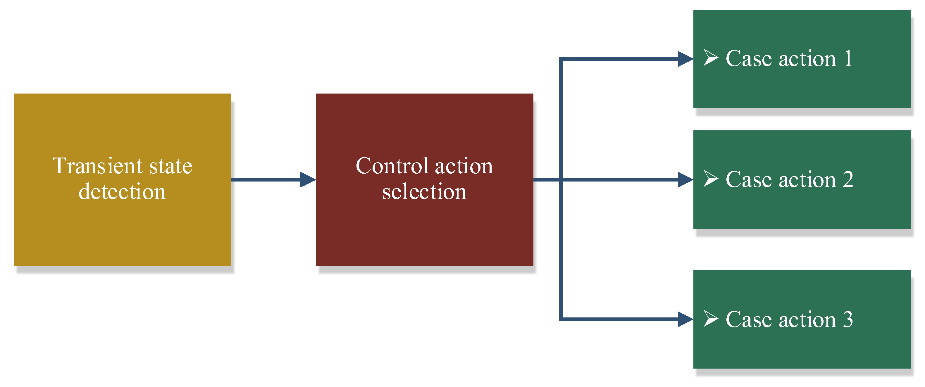
The proposed algorithm, shown in Figure 12 and Figure 13, is separated into two main steps, explained in detail later. To avoid entering the overmodulation control loop in transient time, where the modulator may be out of range momentarily, the following sentence is first encountered:

$$\begin{array}{l}f\left(\left|\frac{1}{L}{G}_{ac}{m}^{dq}{v}^{dc}-\frac{R}{L}{i}_s{}^{dq}-W{i}_s{}^{qd}-\frac{1}{L}{v}_s{}^{dq}\right|<\epsilon \right)\\ Transient=1\\ else\\ Transient=0\end{array}$$

(33)

where ε = [ε₁ ε₂]^T and ε₁, ε₂ are parameters to be syntonized, and for the experimental setup, a value of 5 × 10⁻³ was used. If the condition in (33) is met, it can be said that the system is in a steady-state condition.

In order to avoid changing from step to step at all time, the algorithm will pass to the next step only if the “count” reaches “Time_wait”, raising the Action Time Control (ATC) flag “Flag_ATC” (see Figure 12) and giving enough time to reach the steady-state condition, avoiding oscillations between the steps and cases (presented later), where “Time_wait” is a tuning parameter.

Given that the proposed control strategy is based on the exact value of the modulator M^dq, a low-pass filter must be implemented to attenuate undesirable noise for this variable:

$$M_f\left(k\right)=e^{-\frac{\frac{1}{N\cdot 50}}{70m}}{M}_f\left(k-1\right)+\left(1-e^{-\frac{\frac{1}{N\cdot 50}}{70m}}\right)M^{dq}\left(k\right)$$

(34)

Using N = 204 from PLL algorithm, it is obtained:

$$M_f\left(k\right)=0.9986\cdot M_f\left(k-1\right)+0.0014\cdot M^{dq}\left(k\right)$$

(35)

Overmodulation Control Step by Step

• First Step: The first step looks for overmodulation, (12), while the power converter is in normal operation. If the filtered signal M_f is greater than M_max, the first action is to enlarge the operating region by changing the power factor to 0.96 inductive, which gives room for the second step.
• Second Step: The second step is activated only when the First Step has already been activated (in Figure 13 related to “Step == 1”), and it is divided into three cases:

  ○

  Case 1: If the filtered M_f is greater than the maximum value M_max, then the worst state is happening. MPPT is deactivated to increase the voltage and therefore increase the operating region, such that:

  $$v^{dc}{}_{ref}\left(k\right)=v^{dc}{}_{ref}\left(k-1\right)+T_i{}^{ro}\left(1+{\Delta }^{ro}\right)v^{dc}{}_{ref}\left(k-1\right)$$

  (36)

  In addition, the power factor is kept at 0.96 inductive.

  ○

  Case 2: When the filtered M_f is within the range [M_sub-max∙M_max, M_max], where M_sub-max is an adjustable parameter of sub maximum. For this work, a value of M_sub-max = 0.9 is used. Then, the system is kept in the actual position since it is possible that the problem (over voltage or over frequency) is still ongoing.

  ○

  Case 3: If the filtered M_f is below M_sub-max∙M_max, then it is said that the system is out of trouble and can return to normal operation. Therefore, the MPPT is reactivated, the power factor is set to unity, and the “look up Step 1” is activated.

Thus, the aforementioned algorithm is able to deal with the overmodulation caused by grid disturbances.

6.6. Overmodulation Control Based on Operation Region

The primary advantages of the algorithm lie in its ease of implementation and the ability to be integrated with other injection-control techniques, with the goal of delivering greater stability to the grid. Conversely, a major disadvantage in its implementation is the high total computation time required for all associated strategies in systems characterized by imbalanced amplitude and a wide frequency range. However, the proposed strategy is characterized by low cost, which served as a focal point for improvement during the implementation process.

Table 3. Comparative table.

	[31]	[32]	[33]	Proposed Algorithm
Difficulty of Implementation	Medium	Medium	Medium	Low
Computing Time	Medium	Medium	High	Low
Modular Capacity	yes	No	Yes	Yes
Dependent on Topology (VSC CSC)	Yes	Yes	Yes	No
Load/Generation Usage	Load	Generation? (Inverter)	Generation (inverter)	Generation

illustrates the advantages and disadvantages of comparing the proposed algorithm with others found in the literature.

In [31], The paper discusses different overmodulation strategies used in modern space vector PWM converters, analyzing their voltage transfer ratio (VTR) and low-order harmonics. The complexity of the modulation algorithm is elaborated, and the accuracy and linearization of the VTR are obtained through Fourier transform analysis. The current paper is appended to the table with the primary objective of categorizing all the strategies in comparison with the proposed approach presented in this study.

In [32], an improved overmodulation strategy is proposed for a 3L-NPC-VSI in a maglev traction system. The strategy, based on the minimum amplitude error method, increases DC-bus voltage utilization and adopts a virtual space vector modulation strategy for NP voltage balance, CMV suppression, and leakage current suppression.

In [33], a simple formulation of the virtual-vector-based PWM strategy for multilevel three-phase neutral-point-clamped (NPC) DC-AC converters is presented. The algorithm maintains capacitor voltage balance in every switching cycle and is applicable to any number of levels and operating conditions, including overmodulation. Simulation results confirm the effectiveness of the proposed formulation. This paper provides a comprehensive, effective, and simple PWM formulation for multilevel, three-phase NPC DC–AC converters.

The aforementioned studies are summarized in Table 3.

7. Results

This section presents the simulated and experimental results related to the proposed algorithm for microgrids and weak-grid systems with larger variations in their quantities, such as frequency and amplitude in the grid voltage.

7.1. Simulation Results

Simulations are performed in PSim^® software, and the parameters are listed in

Table 4. Simulation parameters.

Parameter	Value
Inverter and grid
Vs (Grid voltage)	380 Vrms
R (Inductive losses)	0.4 Ω
L (Inductive filter)	7 mH
Cdc (DC-link filter)	2.35 mF
S (Standard operating condition)	1000 W/m2
T (Standard operating condition)	25 °C
pf (Nominal power factor)	1
PV Array
Rs (Series resistance)	8 mΩ
Rsh (Shunt resistance)	1000 Ω
I0 (Short circuit current)	3.8 A
IS0 (Saturation current)	216 µA
n (Ideality factor)	1.2 p.u
Ct (Temperature coefficient)	0.0024

. The main waveforms of the simulation that validate the mathematical analysis of the photovoltaic system are shown in Figure 14.

Figure 14a shows the variation in the overmodulation indicator, which exceeds the maximum value, M_max, when the frequency goes from 50 to 90 Hz at t = 0.3 s. Under this condition, the algorithm first generates a new reference in the pf, as shown in Figure 14b. However, it is not sufficient to reduce the overmodulation indicator. Then, the second action is to increase the reference of v^dc, as shown in Figure 14c. After v^dc is increased, the MPP is sacrificed for a short interval of time, until it is visually confirmed that the overmodulation indicator is stable below the configured threshold, as shown in Figure 14d. At approximately t = 0.33 s, the system returns from overmodulation. However, after a given time, and since the system is not out of trouble, the pf returns from unity to 0.96 (inductive), and MPPT is deactivated once again. After the frequency goes down to 50 Hz, the MPPT is reactivated, and the power factor is set to unity again, taking the place of the traditional power converter control. The efficiency of the proposed system is above 94% for currents below 50 A, where losses are considered to be in the IGBTs and in the RL input filter, and inductor losses are considered the most important.

7.2. Experimental Results

The experimental results are obtained from a prototype setup, shown in Figure 15, that emulates the system presented in Figure 1; the system parameters are listed in

Table 5. PV parameters.

Parameter	Value
Inverter and grid
Vs	21 Vrms
R	0.5 Ω
L	12 mH
Cdc	2.35 mF
PV Array (5 panels)
Pmax	10 W
Vmpp	17.8 V
Impp	0.56 A
Voc	21.6 V
Isc	0.61 A

. The hardware setup includes a programmable source California Instruments CSW 5550, a TMS320F28335 DSP-based board, and solar cells. The programable source is employed to simulate the microgrid by varying the frequency and amplitude in the supply voltage to make it possible to popup the proposed algorithm. The CSW 5550 programable source is not regenerative, and therefore a parallel load is required to keep the current flow out from the source at all times. The final implementation diagram is shown in Figure 16, where the load R_L and L_L dissipate the power.

The proposed control validation is obtained from the experimental results of the three cases and is shown in Figure 15. In Figure 17a, the normal operation regime without overmodulation and nominal conditions is shown. In Figure 17b, the system response due to overmodulation produced by an abrupt shift in the grid frequency from 50 to 90 Hz, including a swell in the grid amplitude, is shown. Finally, Figure 17c depicts the system response when the frequency returns to 50 Hz and returns to the state before the disturbance. Thus, it is mandatory to run the overmodulation compensation to counteract the voltage variation. Despite the step change being hard to find in real applications (where changes are softened), it allows us to see the control response performance with a more challenging disturbance, where, as can be seen from results, it has been properly followed by the system.

The results present the expected behavior of the variables for the inverter control. It is observed how the voltage in v^dc increases in an overmodulation situation and then returns when the overmodulation has elapsed. However, these signals alone are not sufficient to validate the operation of the proposed control algorithm. Therefore, to view and validate the proposal, Figure 18 shows the results obtained from the internal variables of the DSC program platform. By including a programmed buffer in the Code Composer Studio (CCS) code, the signals of interest were acquired, displayed, and captured in Figure 18. Figure 18a shows the main internal variables of the CCS. In Figure 18b, M_f is shown, which presents overmodulation when the frequency changes, as shown in Figure 17b. Figure 18e presents the change in the power factor to increase the operating region as the overmodulation goes beyond the limits. In Figure 18d, it is also observed how the voltage acts in order to mitigate the effects on the entire system. In summary, Figure 18 is able to show sequentially the procedure explained in Figure 13. The most important part of Figure 18 is that this plot reveals that the response follows the algorithm’s steps by changing the power factor (disabling the MPPT), then changing the voltage to reach the modulation amplitude that is allowed and settled as M_max. Once the system returns to nominal values, the MPPT is again enabled, together with the power factor (see Figure 17 and Figure 18). Thus, the experimental tests are set up in order to force the system to go into an overmodulation condition and then to be compensated by the designed algorithm. The internal variables (see Figure 18) are of particular interest because they show how the algorithm tries to compensate for the overmodulation by changing the power factor and the DC-link voltage.

8. Conclusions

Microgrids have been shown to exhibit variations in frequency and amplitude due to their low inertia. One of the main problems related to voltage variation is the change in the operating region, which means that the point of operation may fall out of the valid region. Therefore, in this work, an algorithm is proposed to deal with these changes by employing the characteristics of the power converter such as its operating region variation as a function of the power factor and the DC voltage. The control algorithm first includes reactive power to avoid overmodulation while still trying to keep the MPPT working to improve overall system efficiency. However, if this is not sufficient, the next step is to deactivate the MPPT algorithm to increase the DC voltage and therefore increase the operating region, trying to avoid overmodulation. Thus, maximum power extraction is sacrificed for a short period of time.

The algorithm, based on the aforementioned criteria, in conjunction with a nonlinear-based control for the dq-axis currents and PI strategy for the DC voltage, can work in an extended operating region based on the model certainties. The entire system response has satisfactory results in simulations and experiments, extending the operating region by employing the proposed algorithm by around 12% using the first step of reactive power control. Therefore, power converters can be employed in microgrids where amplitude and frequency can vary notably. For future work, it is of interest to implement the proposal in microgrids with an unbalanced system in voltage amplitude. In this way, this proposal contributes to keeping microgrid power generation systems in operation under the most unfavorable conditions, without the need to shut down power due to disturbances.