Article

Soft-Sensor Modeling of Temperature Variation in a Room under Cooling Conditions

1
Organization for Programs on Environmental Sciences, Graduate School of Arts and Sciences, The University of Tokyo, 3-8-1 Komaba, Meguro-ku, Tokyo 153-8902, Japan
2
Technology and Innovation Center, Daikin Industries, Ltd., 1-1 Nishi-Hitotsuya, Settsu, Osaka 566-8585, Japan
*
Author to whom correspondence should be addressed.
Energies 2023, 16(6), 2870; https://doi.org/10.3390/en16062870
Submission received: 15 February 2023 / Revised: 6 March 2023 / Accepted: 17 March 2023 / Published: 20 March 2023

Abstract

:
Non-uniform temperature distributions in air-conditioned areas can reduce the energy efficiency of air conditioners and cause uncomfortable thermal sensations for occupants. Furthermore, it is impractical to use physical sensors to measure the local temperature at every position. This study developed a soft-sensing model that integrates the fundamentals of thermodynamics and transport phenomena to predict the temperature at the target position in space. Water experiments were conducted to simulate indoor conditions in an air-conditioning cooling mode. The transient temperatures of various positions were measured for model training and validation. The velocity vectors of water flow were acquired using the particle image velocimetry method. Correlation analysis of various positions was conducted to select the input variable. The soft-sensing model was developed using the multiple linear regression method. The model for the top layer was modified by the correction of dead time. The experimental results showed the temperature inhomogeneity between different layers. The temperature at each target position under two initial temperatures and two flow rates was accurately predicted with a mean absolute error within 0.69 K. Moreover, the temperature under different flow rates can be predicted with one model. Therefore, this soft-sensing model has the potential to be integrated into air-conditioning systems.

1. Introduction

The emission of large amounts of greenhouse gases, mostly CO2 as a result of world industrialization and the excessive use of non-renewable energy sources, has led to global climate change and serious environmental problems [1]. It is necessary to achieve carbon neutrality, which refers to balancing the emission and removal of CO2, to mitigate the global warming trend [2]. Notably, buildings consume a lot of energy and contribute to about one-third of global CO2 emissions [3]. As global temperatures rise, the demand for indoor cooling systems will increase their subsequent energy consumption, especially in some hot and densely populated zones, such as South and Southeast Asia [4]. In Singapore, electricity consumption for cooling can account for 60% of the building sector [5]. Increasing the efficiency of energy utility is one of the effective ways to reduce carbon emissions [6]. Therefore, reducing energy consumption in an air-conditioning cooling model can contribute to carbon neutrality.
Conventional fixed-frequency air conditioners use an ON/OFF control scheme to introduce cooled or uncooled air into the room based on feedback from a temperature sensor installed inside the unit [7]. However, the distribution of indoor temperature is not uniform in the air-conditioning zones [8]. The temperature difference in the vertical direction is often larger than in the horizontal direction [9]. Furthermore, the low energy efficiency of air conditioners and uncomfortable thermal sensations for occupants are caused by unevenly distributed indoor local temperatures [10]. However, it is impractical to install a large number of physical sensors in a room to measure local temperatures. Therefore, the accurate and rapid prediction of indoor local temperatures is the first step toward the more effective control of air-conditioning systems, resulting in better human comfort and more efficient energy utility.
Because of the limitations of physical sensor installation and economics, soft sensors are becoming more widely used [11]. Soft sensors are mathematical models that use easy-to-measure variables to predict hard-to-measure variables [12]. New real-time information about the process is created by the combination of analytical hardware data and mathematical models [13].

1.1. Literature Review

Recently, some reports have focused on the applications of soft sensors in heating, ventilation, and air-conditioning systems. Vadamalraj et al. [14] designed a hybrid ventilation system implemented by soft sensors and predictive control. The cooling load and indoor air quality were predicted using soft sensors based on neural networks. Ran et al. [15] developed a virtual flowmeter model based on energy and flow balance to predict the flow rate of water in individual air-handling units. Alonso et al. [16] estimated cooling production and assessed the coefficient of performance in chillers by employing a soft-sensor model based on the electric power, gas temperatures, and gas pressures in each refrigeration circuit. The separable 2D convolutional neural network method was selected to build the soft sensor after comparing six modeling approaches.
Moreover, some researchers have focused on using soft sensors to forecast indoor temperatures. Attoue et al. [17] predicted indoor temperatures in an old building using an artificial neural network model that considered outdoor conditions. A relevance analysis of many input parameters was conducted to select pertinent input parameters. Xu et al. [18] proposed a new deep learning model based on long short-term memory to predict indoor temperatures in public buildings. The long short-term memory model was revised by incorporating error correction, and the directional forecasting accuracy was significantly improved. Candanedo et al. [19] proposed a random forest model and a multiple linear regression model to reconstruct the database of indoor temperatures for a passive house based on incomplete data. Two regression models were evaluated using the root-mean-square error as a key performance indicator.
As can be seen from the literature, the above studies incorporated fewer process mechanisms in the building and analysis of soft-sensor models used to predict indoor temperatures in air-conditioning areas. They focused more on the data-driven model without any process mechanism. Moreover, they did not focus on the prediction of the local temperature at a point (including the horizontal and vertical directions) in the room. In our previous work [20], we proposed a multiple linear regression model for predicting temperature changes at target points under cooling conditions. However, temperature hysteresis of the top layer affected the model accuracy. Further investigation is necessary to find a correction method for precision improvement. Overall, soft sensors exhibit the potential for monitoring local temperatures in air-conditioning areas.

1.2. Research Objective and Paper’s Organization

In this paper, a soft sensor that can forecast the real-time indoor local temperature in an air-conditioning cooling model was further investigated. The major contributions of this study are summarized as follows:
  • A new soft-sensor model used to predict the transient local temperature at the target position in space is developed based on the heat transfer process mechanism, and the effects of fluid transport on the temperature variations and model coefficients are understood by the flow visualization;
  • The transient local temperature of each target position is accurately predicted by the proposed model. The accuracy of the model for the top layer is improved by a dead time correction;
  • The model accuracy is barely affected within a 10% flow rate difference. The efforts in the soft sensor development of the air-conditioner system in practice can be reduced.
This paper is organized as follows: The next section introduces the experimental setup and methods for temperature data collection and flow visualization, as well as the multiple linear regression model used in this study. Subsequently, the experimental results of temperature variation and flow visualization, as well as the results of model training and validation, are presented and discussed. Conclusions are given at the end of this paper.

2. Methodology

The research methodology of this paper follows our previous work [20]. For the experiments, the state of indoor air in the air-conditioning cooling model was simulated by the temperature change and flow state of water in an enclosed space. The collected temperature data were used for model training and validation. The velocity field was investigated by visualizing the flow to explain the effects of fluid transport on the temperature variations and model coefficients.

2.1. Experimental Setup and Methods

A schematic of the experimental setup for temperature data collection is shown in Figure 1. A water circulator (No. 1) was used for heating, cooling, and circulation of water. Water in an acrylic box (No. 6) was initially adjusted to a constant designated temperature, the initial temperature, to simulate the initial state of the air-conditioned room. After the cold water in a water container (No. 4) reached a constant designated temperature, the feed temperature, the cold water was continuously supplied to the acrylic box through a feed nozzle (No. 7) to simulate the operating state of the air-conditioning cooling model. The excess water in the acrylic box was removed by an aspirator (No. 9) through a drain nozzle (No. 8) and discharged into a recovery container (No. 10). A three-way valve (No. 5) was used to control the start and stop of the water supply. Two needle valves (No. 2) were used to adjust the flow rate. In addition, 39 K-type thermocouples (13 horizontal × 3 vertical) were installed at different locations inside the acrylic box for temperature collection. Figure 1b,c show the specific positions of thermocouples, with an equal distance between different layers and symmetrical distribution at the same layer. The acrylic box was wrapped with thermal insulation, and the interior of the box was fitted with thermal insulation to simulate the ceiling. The thermal conductivity of thermal insulation was 0.028 W/(m·K). The feed temperature was measured using a K-type thermocouple in the feed nozzle. The experimental conditions for temperature data collection were set as follows: the initial temperatures were 25 and 35 °C, the feed temperature was 10 °C, the flow rates were 770 and 850 mL/min, and the sampling time was 100 ms.
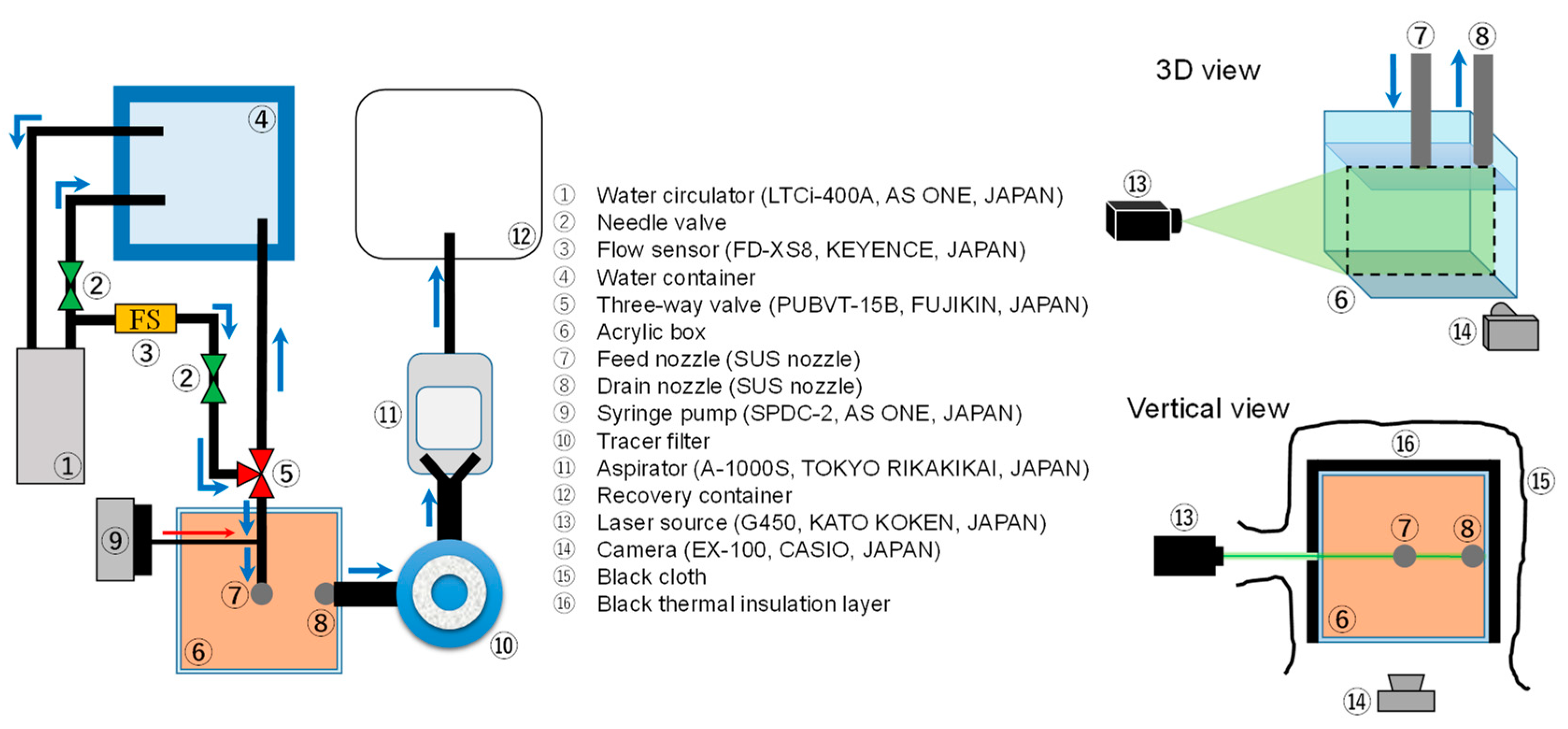
A schematic of the experimental setup for flow visualization is shown in Figure 2. The main difference compared with the temperature data collection setup was the addition of a tracer filter (No. 10), a syringe pump (No. 9), a laser source (No. 13), and a camera (No. 14). The water circulation method of flow visualization was the same as that of the temperature data collection. The tracer particle flowed into the feed water using the syringe pump. The central cross-section of the acrylic box (entire C surface) was vertically illuminated by the laser source. The illuminated surface was observed using the camera installed in front of the acrylic box. The flow regime was analyzed using the particle image velocimetry (PIV) method (PIV software: FLOW EXPERT 2D2C Ver.1.3.3.1, Kato Koken, Japan). The experimental conditions of flow visualization were set as follows: the tracer particle was a fluorescent red polyethylene microsphere (UVPMS-BR-0.995, COSPHERIC LLC, USA) with a diameter of 75–90 µm and a density of 0.995 g/cm3, the frame rate of the video was 120 fps, the initial temperatures were 25 and 35 °C, the feed temperature was 10 °C, and the flow rate was 770 mL/min.

2.2. Mathematical Model

Multiple linear regression is a statistical method used for describing the simultaneous relationships of multiple variables with one continuous outcome, and the model is expressed as follows [21]:
y = β 0 + β 1 x 1 + + β n x n + ε  
where y is the dependent variable, and x is the independent variable. This approach provides a more accurate understanding of the relationship between each independent variable and the outcome, as well as the relationships among independent variables [22]. Considering the computational cost and speed, as well as the simplicity of the model, a multiple linear regression model was used for temperature prediction. In this research, independent variables are easy-to-measure data and the dependent variable is hard-to-measure data. It is not possible to install a new physical sensor in the interior space of the room; however, it can be mounted on the wall. Thus, the temperatures of locations on the wall of the acrylic box, such as C1, E1, D1, and so on, are the candidates of an input variable. The correlation coefficients between temperatures at different locations are calculated for variable selection, as follows:
r X Y = 1 n i = 1 n X i X ¯ Y i Y ¯ 1 n i = 1 n X i X ¯ 2 1 n i = 1 n Y i Y ¯ 2
where rXY is the correlation coefficient, X i and X ¯ are the ith temperature data and mean temperature data at a certain position, respectively, and Y i and Y ¯ are the ith temperature data and mean temperature data at another position, respectively. The temperature prediction model was built based on the heat transfer process mechanism according to Newton’s law of cooling and Fourier’s law of heat conduction, as follows:
T p r e d i c t e d = a + b T m e a s u r e d + c T m e a s u r e d T s + d d T m e a s u r e d d t
where Tpredicted is the predicted temperature at the target location; Tmeasured is the measured temperature, which is the variable selected by the correlation analysis; Ts is the feed temperature, TmeasuredTs is the convective heat transfer term; dTmeasured/dt is the assumption for heat conduction obtained by polynomial fitting in a variation of the measured temperature; and a represents the influence or error caused by other parameters, such as radiation. After arrangement, the final model is shown in the following equation:
T p r e d i c t e d = α + β T m e a s u r e d + γ T s + δ d T m e a s u r e d d t
where α, β, γ, and δ are model coefficients calculated using the least squares method with the training data. The experimental data at a given location, which has the same distance from the wall and feed nozzle as the corresponding location in the training data, are chosen for model validation. The assumptions of the proposed model are linearity, absence of multicollinearity, normal distribution, and freedom from extreme values [21]. Notably, Tmeasured, Ts, and dTmeasured/dt are not independent variables. However, the presence of the predictor variables that are correlated among them does not affect the prediction accuracy and goodness-of-fit of the model when the purpose of the model is for prediction [23].

3. Results and Discussion

3.1. Experiments

3.1.1. Temperature Variation

As shown in Figure 1b,c, A1, A2, A3, B1, B2, and so on represent the specific position in the horizontal direction, and the suffixes T (top), M (middle), and B (bottom) represent the position in the vertical direction. The typical temperature variation comparisons between E1T, E1M, and E1B are shown in Figure 3. It takes about 600 s for the initial temperature of 25 °C and about 700 s for the initial temperature of 35 °C to reach homogeneity between layers. Before the temperature of each layer becomes consistent, the temperature difference between the middle layer and the bottom layer is smaller, and the temperature difference between the top layer and the other layers is larger. A temperature-drop hysteresis occurs in the top layer at the initial stage. This period without any response is called dead time [24]. In this system, the elapsed time when the temperature variation rate reaches a preset threshold for the first time is defined as dead time. The temperature inhomogeneity is more obvious at the initial temperature of 35 °C compared with 25 °C because of the greater temperature difference between the feed and initial temperatures.
Moreover, the temperature variation trends at other locations are similar to E1, in addition to C2, A1, A3, and C3T. The temperature drops faster in each layer of C2, and there is no hysteresis in the temperature drop in the top layer because C2 is located directly below the feed nozzle. The temperatures of A1B and A3B located in the corner of the acrylic box decrease slower than A1M and A3M. Compared with C1T, C3T has a faster response with a shorter dead time because the location is very close to the drain nozzle.
The typical temperature variation comparisons between different flow rates of 770 and 850 mL/min at the initial temperature of 35 °C are shown in Figure 4. There is no difference in temperature responses between different flow rates in the middle and bottom layers. However, in the top layer, the temperature at the flow rate of 850 mL/min decreases faster with a shorter dead time compared with 770 mL/min. The decrease in dead time is caused by enhanced fluid transport at the increased flow rate [24]. These phenomena are also observed using the initial temperature of 25 °C.

3.1.2. PIV Analysis

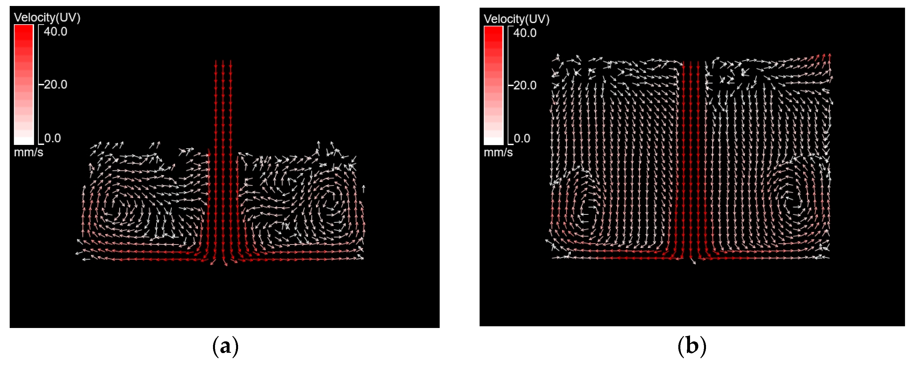
The PIV method was used to obtain mean velocity vectors at the flow rate of 770 mL/min. Figure 5 shows the mean velocity vectors obtained under the initial temperature of 35 °C. Cold water flowing out from the feed nozzle first reaches the bottom surface and flows along the bottom surface to the wall surface, and symmetrical vortices are formed after touching the wall surface. Forced convection plays a dominant role in the middle and bottom layers. Moreover, the flow velocity along the bottom layer is larger than that along the wall surface and in the vortices. At the elapsed time of 90 s, there are only a few or no random velocity vectors above the middle layer, which corresponds to a delayed response in the top layer. This region is considered to be dominated by natural convection and heat conduction. At the elapsed time of 540 s, the vectors become ordered and fill the space. The temperature tends to be homogeneous between the layers. Moreover, fluid transport at the location close to the drain nozzle is accelerated by water suction, resulting in a faster C3T response.

3.2. Model Training and Validation

3.2.1. Correlation Analysis

According to the results of the correlation analysis, the transient temperature at C1M has a significant positive linear correlation with the transient temperature at each location. The correlation coefficients of the transient temperature at C1M with transient temperatures at partial locations are shown in Table 1. In addition, physical sensors for online data collection can be integrated into the remote control panel of the air conditioner located in the middle of the room’s wall. This has the advantages of space and cost savings. Thus, the measured data of C1M are chosen as input data.

3.2.2. Case Study

The model is divided into sub-models according to different locations and different experimental conditions. The C1M-B1M model is acquired by calculating the coefficients of Equation (4) using the experimental data of C1M and B1M as training data. The C1M-B1M model under the initial temperature of 35 °C at the flow rate of 770 mL/min is expressed as follows:
T B 1 M t = 0.536 + 0.916 T C 1 M t + 0.090 T s t 14.380 d T C 1 M t d t
where TB1M(t) is the transient temperature of B1M, TC1M(t) is the transient temperature of C1M, and Ts(t) is the transient feed temperature. The position of B2M is similar to B1M, and the position of A2M is similar to C1M. Thus, the transient temperature of B2M is predicted using the experimental data of A2M and the coefficients of Equation (5) to validate the C1M-B1M model, as follows:
T B 2 M t = 0.536 + 0.916 T A 2 M t + 0.090 T s t 14.380 d T A 2 M t d t
where TB2M(t) is the transient temperature of B2M, and TA2M(t) is the transient temperature of A2M. The coefficient of determination (R2), the temperature difference between experimental data and predicted data (ΔT), and the mean absolute error (MAE) are used to evaluate the model accuracy, and they are expressed as follows:
R 2 = 1 i = 1 n y i y ^ i 2 i = 1 n y i y ¯ i 2
Δ T i = y i y ^ i
MAE = i = 1 n y i y ^ i n
where y i , y ^ i , and y ¯ i are experimental data, predicted data, and the mean value of experimental data, respectively.
The training data at B1M are fitted well by the C1M-B1M model, with an R2 value of 0.993. The validation result of the C1M-B1M model is shown in Figure 6. The experimental data of B2M agree well with the predicted data, with an MAE value of 0.38 K. ΔT can be controlled within about ±1 K. Therefore, good accuracy is obtained by the C1M-B1M model under the initial temperature of 35 °C and flow rate of 770 mL/min.
For the middle layer at other locations, the bottom layer, and different initial temperatures, the model is obtained using the same method. The coefficients, R2, and MAE of the model for the middle layer and bottom layer under the initial temperatures of 25 and 35 °C are summarized in Table 2. The R2 values of 0.975–0.997 and MAE values of 0.15–0.69 K demonstrate the acceptable accuracy of the model for the middle layer and bottom layer under the two initial temperatures of 25 and 35 °C. γ is the coefficient of Ts, which is related to the convection. At the same initial temperature, the coefficient γ in the bottom layer is higher than that in the middle layer. This means that the bottom layer is more strongly influenced by convection, which corresponds with the higher flow velocity in the bottom layer, as observed by PIV analysis. However, A1B is a special case because of the location in the corner, where fluid transport is difficult.
A multiple linear regression model used to predict the real-time indoor temperature in a mobile container was reported [25]. The wind speed, environment temperature, global solar irradiance, and modeled indoor temperature at the previous time step were used as inputs. The results showed that the MAE values in the two validation cases for predicting the indoor temperature of two validated days were 0.28 and 0.49 K, respectively. The models and validation results of the above study are similar to our study; however, the proposed model in our study was trained and validated by the experimental data from water experiments. The density of water is much larger than that of air, and the heat transfer rate is much slower. Therefore, the model is substantially different from the proposed one. Moreover, the study did not focus on the local temperature [25].

3.2.3. Dead Time Correction

Training data of the top layer, including dead time, cannot be fitted well by the model using the above method. One reason is that the differential term in the model cannot fit the almost constant temperature during dead time. Another reason is that the response of the top layer is delayed by a dead time compared with the input data, resulting in an unsynchronized response. It is necessary to eliminate the effect of dead time on the model for the top layer to improve accuracy. Thus, the model for the top layer is modified by dividing it into a dead time part and a response part. The C1M-B1T model under the initial temperature of 35 °C and flow rate of 770 mL/min is given by the following equation:
T B 1 T t = T i n i t i a l ( 0 t < t 0 ) T B 1 T t = 2.249 + 0.850 T C 1 M t t 0 + 0.201 T s t t 0 2.494 d T C 1 M t t 0 d t ( t t 0 )
where TB1T(t) is the transient temperature of B1T, t0 is the dead time, and Tinitial is the initial temperature. The response of B1T is shifted forward by a dead time. The experimental data of B2T, with a similar position to B1T, are used for validation. Model training and validation of the top layer at location B are shown in Figure 7. The coefficients, R2, and MAE of the model for the top layer at the initial temperatures of 25 and 35 °C are summarized in Table 3. An acceptable accuracy, with the MAE values of 0.27–0.63 K, is obtained after correcting for the dead time. Moreover, the γ becomes too high for the top layer after removing the dead time.

3.2.4. Model Comparison between Different Flow Rates

The model with the flow rate of 850 mL/min is obtained using the same method as that of 770 mL/min. The coefficients, R2, and MAE of the model at the flow rate of 850 mL/min are shown in Table S1 of Supplementary Materials. The R2 values of 0.977–0.998 and MAE values of 0.15–0.62 K demonstrate the acceptable accuracy of the model at the flow rate of 850 mL/min.
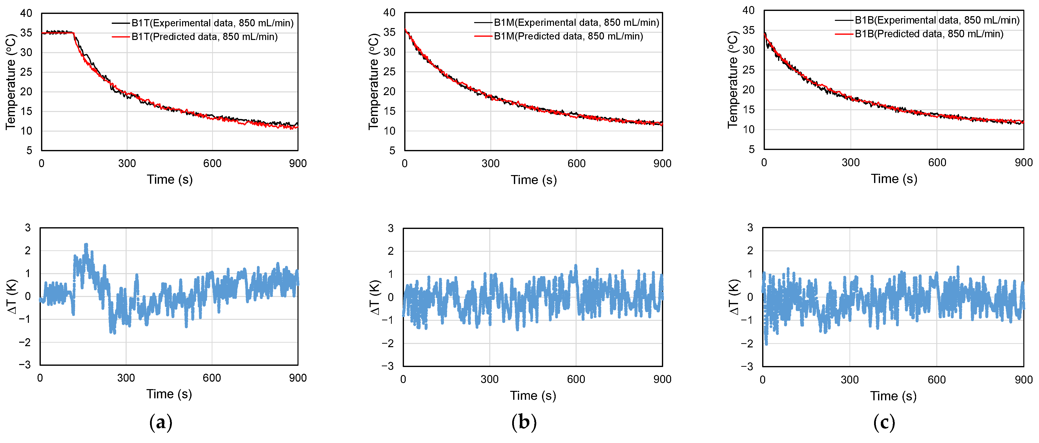
Figure 8 shows the results of using the model for 770 mL/min to predict the experimental data of 850 mL/min. The MAE values of B1T, B1M, and B1B at the initial temperature of 35 °C are 0.55 K, 0.42 K, and 0.43 K, respectively. At the same time, the experimental data of 770 mL/min are predicted by the model for 850 mL/min. The MAE values of B1T, B1M, and B1B at the initial temperature of 35 °C are 0.50 K, 0.42 K, and 0.42 K, respectively. Both validations using the model for one flow rate to predict the experimental data of another flow rate have acceptable accuracy. In the case of a 10% difference between the flow rates, it can be considered to use one model for prediction.

4. Conclusions

This paper proposed a soft sensor built using an experimental investigation and multiple regression analysis to predict the local transient temperature. Temperature measurements and flow visualization in an enclosed space were conducted under various conditions using different initial temperatures (25 and 35 °C) and flow rates (770 and 850 mL/min). A multiple linear regression model was developed based on heat transfer processes, which we combined with correlation analyses of different locations to determine the input variable, which was trained and validated using the experimental data. The PIV analysis provided an understanding of the effects of fluid transport on temperature variations and model coefficients. The model accuracy was evaluated using the indicators of R2, ΔT, and MAE. The model of each target location demonstrated good accuracy with the MAE values within 0.69 K for multiple initial temperatures and flow rates. For the top layer, the dead time correction was used to improve the model. Furthermore, the experimental data of one flow rate were predicted well by the model of another flow rate and vice versa. Within a 10% difference in flow rates, one model is recommended to predict the temperature change at different flow rates This means that the model accuracy is hardly affected when the air conditioner’s airflow is slightly adjusted or when the airflow fluctuates because of disturbances, such as dust.
By integrating this fast-response soft sensor into the control system of the air conditioner, optimal control can be realized by the accurate prediction of local temperatures to maintain efficient energy management and human comfort. Therefore, this study has great potential to contribute to the development of air-conditioner systems. In future work, it is necessary to assess the performance of the soft-sensing model for monitoring heating conditions, especially because heating modes typically require more energy and receive more thermal complaints than cooling modes.

Supplementary Materials

The following supporting information can be downloaded at: https://www.mdpi.com/article/10.3390/en16062870/s1. Table S1. The coefficients, R2, and MAE of the model at the flow rate of 850 mL/min.

Author Contributions

Conceptualization, F.X. and Y.K.; methodology, F.X., K.S., Y.S. (Yuki Sato), Y.S. (Yuka Sakai), S.S., H.K., D.S. and Y.K.; validation, F.X., K.S., Y.S. (Yuki Sato), Y.S. (Yuka Sakai), S.S., H.K. and D.S.; formal analysis, F.X., K.S., Y.S. (Yuki Sato) and Y.S. (Yuka Sakai); investigation, F.X., K.S., Y.S. (Yuki Sato), Y.S. (Yuka Sakai), S.S., H.K., D.S. and Y.K.; data curation, F.X., K.S., Y.S. (Yuki Sato) and Y.S. (Yuka Sakai); writing—original draft preparation, F.X. and Y.K.; writing—review and editing, F.X. and Y.K.; visualization, F.X., K.S., Y.S. (Yuki Sato) and Y.S. (Yuka Sakai); supervision, Y.K.; project administration, Y.K.; funding acquisition, Y.K. All authors have read and agreed to the published version of the manuscript.

Funding

The New Energy and Industrial Technology Development Organization (NEDO), JPNP20004.

Data Availability Statement

Data are contained within the article and Supplementary Materials.

Acknowledgments

This paper is based on results obtained from a project, JPNP20004, subsidized by the New Energy and Industrial Technology Development Organization (NEDO).

Conflicts of Interest

The authors declare no conflict of interest.

Nomenclature

MAEMean absolute error
rXYCorrelation coefficient
R2Coefficient of determination
t0Dead time, s
TinitialInitial temperature, °C
TmeasuredMeasured temperature, °C
TpredictedPredicted temperature, °C
TsFeed temperature, °C
ΔTTemperature difference between experimental data and predicted data, K
xDependent variable
X i ,   X ¯ ith temperature data and mean temperature data at a certain position for correlation analysis
Y i ,   Y ¯ ith temperature data and mean temperature data at another position for correlation analysis
yIndependent variable
y i Experimental data
y ^ i Predicted data
y ¯ i Mean value of experimental data
α, β, γ, δCoefficients of the mathematical model

References

  1. Chen, L.; Msigwa, G.; Yang, M.; Osman, A.I.; Fawzy, S.; Rooney, D.W.; Yap, P.-S. Strategies to Achieve a Carbon Neutral Society: A Review. Environ. Chem. Lett. 2022, 20, 2277–2310. [Google Scholar] [CrossRef] [PubMed]
  2. Yu, F.W.; Ho, W.T. Tactics for Carbon Neutral Office Buildings in Hong Kong. J. Clean. Prod. 2021, 326, 129369. [Google Scholar] [CrossRef]
  3. Wang, N.; Phelan, P.E.; Harris, C.; Langevin, J.; Nelson, B.; Sawyer, K. Past Visions, Current Trends, and Future Context: A Review of Building Energy, Carbon, and Sustainability. Renew. Sustain. Energy Rev. 2018, 82, 976–993. [Google Scholar] [CrossRef]
  4. Lundgren, K.; Kjellstrom, T. Sustainability Challenges from Climate Change and Air Conditioning Use in Urban Areas. Sustainability 2013, 5, 3116–3128. [Google Scholar] [CrossRef] [Green Version]
  5. Li, X.-X. Linking Residential Electricity Consumption and Outdoor Climate in a Tropical City. Energy 2018, 157, 734–743. [Google Scholar] [CrossRef]
  6. Chen, J.M. Carbon Neutrality: Toward a Sustainable Future. Innovation 2021, 2, 100127. [Google Scholar] [CrossRef] [PubMed]
  7. Cheng, C.-C.; Lee, D. Smart Sensors Enable Smart Air Conditioning Control. Sensors 2014, 14, 11179–11203. [Google Scholar] [CrossRef] [PubMed]
  8. Yang, Z.; Dong, X.; Xiao, H.; Sun, H.; Wang, B.; Shi, W.; Li, X. Investigation of Thermal Comfort of Room Air Conditioner during Heating Season. Build. Environ. 2022, 207, 108544. [Google Scholar] [CrossRef]
  9. Zhang, H.; Arens, E.; Zhai, Y. A Review of the Corrective Power of Personal Comfort Systems in Non-Neutral Ambient Environments. Build. Environ. 2015, 91, 15–41. [Google Scholar] [CrossRef] [Green Version]
  10. Yang, Z.; Xiao, H.; Sun, H.; Wang, B.; Lin, B.; Shi, W.; Huang, W. Performance Analysis of Room Air Conditioners via Questionnaire and Integrated Field Test. Appl. Therm. Eng. 2021, 196, 117243. [Google Scholar] [CrossRef]
  11. Jiang, Y.; Yin, S.; Dong, J.; Kaynak, O. A Review on Soft Sensors for Monitoring, Control, and Optimization of Industrial Processes. IEEE Sens. J. 2021, 21, 12868–12881. [Google Scholar] [CrossRef]
  12. Souza, F.A.A.; Araújo, R.; Mendes, J. Review of Soft Sensor Methods for Regression Applications. Chemom. Intell. Lab. Syst. 2016, 152, 69–79. [Google Scholar] [CrossRef]
  13. Randek, J.; Mandenius, C.-F. On-Line Soft Sensing in Upstream Bioprocessing. Crit. Rev. Biotechnol. 2018, 38, 106–121. [Google Scholar] [CrossRef]
  14. Vadamalraj, N.; Zingre, K.; Seshadhri, S.; Arjunan, P.; Srinivasan, S. Hybrid Ventilation System and Soft-Sensors for Maintaining Indoor Air Quality and Thermal Comfort in Buildings. Atmosphere 2020, 11, 110. [Google Scholar] [CrossRef] [Green Version]
  15. Ran, F.; Gao, D.; Zhang, X.; Chen, S. A Virtual Sensor Based Self-Adjusting Control for HVAC Fast Demand Response in Commercial Buildings towards Smart Grid Applications. Appl. Energy 2020, 269, 115103. [Google Scholar] [CrossRef]
  16. Alonso, S.; Morán, A.; Pérez, D.; Prada, M.A.; Díaz, I.; Domínguez, M. Estimating Cooling Production and Monitoring Efficiency in Chillers Using a Soft Sensor. Neural Comput. Appl. 2020, 32, 17291–17308. [Google Scholar] [CrossRef]
  17. Attoue, N.; Shahrour, I.; Younes, R. Smart Building: Use of the Artificial Neural Network Approach for Indoor Temperature Forecasting. Energies 2018, 11, 395. [Google Scholar] [CrossRef] [Green Version]
  18. Xu, C.; Chen, H.; Wang, J.; Guo, Y.; Yuan, Y. Improving Prediction Performance for Indoor Temperature in Public Buildings Based on a Novel Deep Learning Method. Build. Environ. 2019, 148, 128–135. [Google Scholar] [CrossRef]
  19. Candanedo, L.M.; Feldheim, V.; Deramaix, D. Reconstruction of the Indoor Temperature Dataset of a House Using Data Driven Models for Performance Evaluation. Build. Environ. 2018, 138, 250–261. [Google Scholar] [CrossRef]
  20. Xu, F.; Sato, Y.; Sakai, Y.; Sabu, S.; Kanayama, H.; Satou, D.; Kansha, Y. A Prediction Model for Temperature Variation and Distribution Using Soft Sensing Method. Chem. Eng. Trans. 2022, 94, 811–816. [Google Scholar] [CrossRef]
  21. Uyanık, G.K.; Güler, N. A Study on Multiple Linear Regression Analysis. Procedia Soc. Behav. Sci. 2013, 106, 234–240. [Google Scholar] [CrossRef] [Green Version]
  22. Marill, K.A. Advanced Statistics: Linear Regression, Part II: Multiple Linear Regression. Acad. Emerg. Med. 2004, 11, 94–102. [Google Scholar] [CrossRef] [PubMed]
  23. Kutner, M.H.; Nachtsheim, C.J.; Neter, J.; Li, W. Applied Linear Statistical Models, 5th ed.; The McGraw-Hill Companies, Inc.: New York, NY, USA, 2005; p. 283. [Google Scholar]
  24. Seborg, D.E.; Edgar, T.F.; Mellichamp, D.A.; Doyle, F.J., III. Process Dynamics and Control, 3rd ed.; John Wiley & Sons, Inc.: Hoboken, NJ, USA, 2011; pp. 82–83. [Google Scholar]
  25. Patonai, Z.; Kicsiny, R.; Géczi, G. Multiple Linear Regression Based Model for the Indoor Temperature of Mobile Containers. Heliyon 2022, 8, e12098. [Google Scholar] [CrossRef] [PubMed]
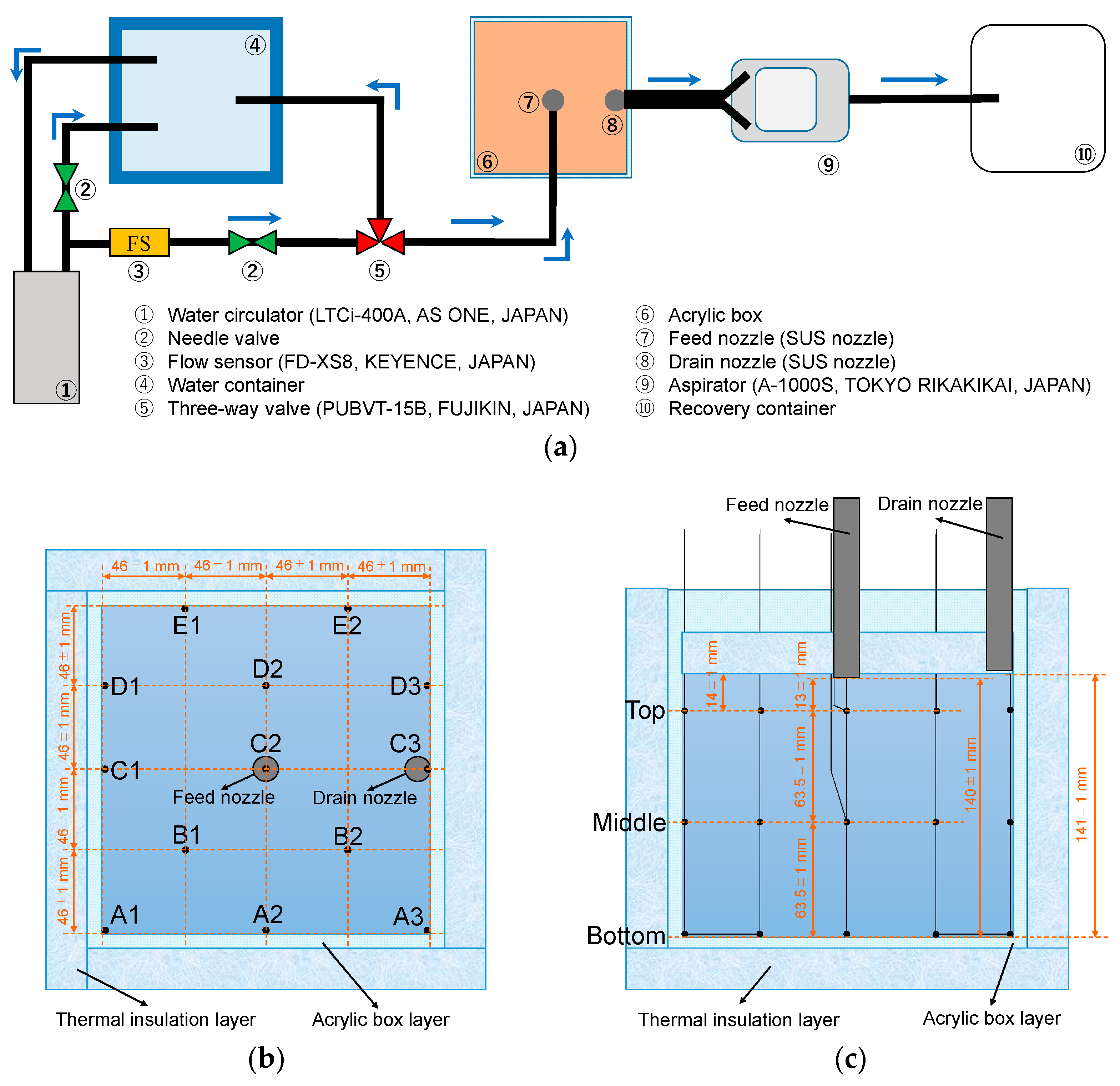
Figure 1. A schematic of the experimental setup for temperature data collection: (a) water circulation system; (b) vertical view of the acrylic box; (c) front view of the acrylic box.
Energies 16 02870 g001
Figure 2. A schematic of the experimental setup for flow visualization.
Energies 16 02870 g002
Figure 3. Temperatures variation comparisons between E1T, E1M, and E1B under the flow rate of 770 mL/min: (a) the initial temperature of 25 °C; (b) the initial temperature of 35 °C.
Energies 16 02870 g003
Figure 4. Temperatures variation comparisons between flow rates of 770 and 850 mL/min at the initial temperature of 35 °C: (a) top layer; (b) middle layer; (c) bottom layer.
Energies 16 02870 g004
Figure 5. Mean velocity vectors under the initial temperature of 35 °C and flow rate of 770 mL/min: (a) the elapsed time of 90 s; (b) the elapsed time of 540 s.
Energies 16 02870 g005
Figure 6. Validation result of C1M-B1M model under the initial temperature of 35 °C and flow rate of 770 mL/min: (a) comparison between predicted and experimental data of B2M; (b) ΔT.
Energies 16 02870 g006
Figure 7. Model training and validation of the top layer at location B under the initial temperature of 35 °C and flow rate of 770 mL/min: (a) training; (b) validation.
Energies 16 02870 g007
Figure 8. The results obtained using the model built at the flow rate of 770 mL/min to predict the data at the flow rate of 850 mL/min under the initial temperature of 35 °C: (a) top layer; (b) middle layer; (c) bottom layer.
Energies 16 02870 g008
Table 1. The correlation coefficients of the transient temperature at C1M with transient temperatures at partial locations under the flow rate of 770 mL/min.
Initial TemperatureB1TB1MB1BD2TD2MD2B
25 °C0.9740.9900.9880.9810.9950.984
35 °C0.9670.9960.9950.9680.9980.993
Table 2. The coefficients, R2, and MAE of the model for the middle and bottom layers at the flow rate of 770 mL/min.
Initial TemperaturePositionαβγδR2MAE (Training)MAE (Validation)
25 °CB1M2.537 0.668 0.066 −87.789 0.982 0.40 0.31
B1B3.000 0.577 0.122 −89.831 0.980 0.38 0.34
A1M2.135 0.886 −0.062 −27.331 0.991 0.28 0.32
A1B4.046 0.902 −0.127 7.548 0.986 0.31 0.31
C1B0.175 0.834 0.155 −9.052 0.996 0.15 0.46
D1M2.915 0.802 −0.042 −54.226 0.982 0.40 0.22
D1B1.091 0.794 0.133 −28.877 0.988 0.31 0.37
E1M3.081 0.755 −0.047 −76.419 0.984 0.38 0.30
E1B−0.251 0.902 0.143 11.478 0.997 0.15 0.32
D2M1.195 0.854 0.030 −38.915 0.990 0.30 0.31
D2B3.130 0.513 0.184 −89.685 0.975 0.41 0.40
35 °CB1M−0.536 0.916 0.090 −14.380 0.993 0.42 0.38
B1B0.964 0.776 0.103 −28.760 0.992 0.40 0.39
A1M0.835 0.984 −0.023 1.074 0.996 0.28 0.42
A1B3.430 0.976 −0.100 21.437 0.995 0.30 0.34
C1B−0.084 0.882 0.131 4.499 0.997 0.23 0.69
D1M0.479 1.006 −0.010 8.852 0.993 0.42 0.25
D1B0.511 0.927 0.056 9.821 0.993 0.36 0.46
E1M0.320 0.982 0.006 2.203 0.992 0.43 0.35
E1B0.274 0.918 0.074 5.558 0.997 0.22 0.37
D2M−0.317 0.963 0.041 −11.902 0.996 0.32 0.39
D2B1.089 0.711 0.164 −31.064 0.990 0.43 0.45
Table 3. The coefficients, R2, and MAE of the model for the top layer at the flow rate of 770 mL/min.
Initial TemperaturePositionαβγδR2 *MAE (Training)MAE (Validation)
25 °CB1T0.693 0.613 0.260 −27.573 0.976 0.33 0.36
A1T7.355 0.333 0.132 −99.007 0.981 0.29 0.29
C1T6.293 0.299 0.124 −143.902 0.988 0.28 0.33
D1T0.777 0.719 0.197 −38.374 0.982 0.33 0.31
E1T6.045 0.293 0.143 −154.540 0.988 0.27 0.30
D2T3.988 0.417 0.173 −129.026 0.985 0.32 0.33
35 °CB1T−2.249 0.850 0.201 −2.494 0.988 0.44 0.63
A1T1.334 0.861 0.135 31.497 0.993 0.33 0.44
C1T−1.602 0.972 0.098 25.296 0.994 0.33 0.42
D1T−1.872 0.967 0.149 29.672 0.992 0.38 0.43
E1T−1.849 0.990 0.093 20.269 0.992 0.39 0.39
D2T−2.435 0.985 0.113 18.534 0.990 0.47 0.50
* The R2 of the model for the top layer is calculated from the response part.
Disclaimer/Publisher’s Note: The statements, opinions and data contained in all publications are solely those of the individual author(s) and contributor(s) and not of MDPI and/or the editor(s). MDPI and/or the editor(s) disclaim responsibility for any injury to people or property resulting from any ideas, methods, instructions or products referred to in the content.