Partial Discharge Localization Techniques: A Review of Recent Progress

Abstract

Monitoring the partial discharge (PD) activity of power equipment insulation is crucial to ensure uninterrupted power system operation. PD occurrence is highly correlated to weakened insulation strength. If PD occurrences are left unchecked, unexpected insulation breakdowns may occur. The comprehensive PD diagnostic process includes the detection, localization, and classification of PD. Accurate PD source localization is necessary to locate the weakened insulation segment. As a result, rapid and precise PD localization has become the primary focus of PD diagnosis for power equipment insulation. This paper presents a review of different approaches to PD localization, including conventional, machine learning (ML), and deep learning (DL) as a subset of ML approaches. The review focuses on the ML and DL approaches developed in the past five years, which have shown promising results over conventional approaches. Additionally, PD detection using conventional, unconventional, and a PCB antenna designed based on UHF techniques is presented and discussed. Important benchmarks, such as the sensors used, algorithms employed, algorithms compared, and performances, are summarized in detail. Finally, the suitability of different localization techniques for different power equipment applications is discussed based on their strengths and limitations.

1. Introduction

The insulation of power equipment plays a crucial role in ensuring the safe and proper operation of the power system. However, power equipment insulation deteriorates over time, and its ageing process is accelerated by abnormal surrounding activities, such as chemical, electrical, and mechanical stresses. These factors ultimately reduce the insulation’s performance [1]. The continual insulation degradation on high-voltage power equipment will lead to a local insulation breakdown known as partial discharge (PD). This phenomenon results from the very irregular distribution of the electric field, which places stress on the insulating components at certain defect spots [2]. Prolonged PD occurrences on the weak points of power equipment insulation can increase the discharge intensity [3] which ultimately leads to catastrophic insulation breakdown [2]. PD diagnostic can be applied to any electrical equipment that has insulation, as long as the PD inception voltage (PDIV) is lower than or equal to its operating voltage [4]. To prevent serious accidents that may cause significant economic losses and threaten the safety and stability of the power system, it is essential to conduct a PD diagnostic test with proper PD source detection, locating the PD sources, and identification of the PD source type in the power system. This will allow for the scheduling of maintenance actions on power equipment [3,5,6]. Based on a case study by a German cable diagnostic company [7], by performing PD testing on a 2.5 km long paper-insulated cable, the faulty segment can be narrowed down to a length of 20 m. Consequently, it is estimated that up to 80% cost savings are possible due to the improved localization of the faulty segment.

Before applying maintenance measures to the correct defect location, it is essential to conduct high-quality PD measurements. During PD activities, commonly emitted signals include electric, electromagnetic, and acoustic signals. Therefore, various PD detection sensors can be utilized in PD condition monitoring, such as high-frequency current transformers (HFCTs), epoxy-mica capacitors, Rogowski coils, UHF, and acoustic sensors [8]. PD measurement, defined using IEC-60270 [2] and IEC-62478 [9] standards, includes conventional techniques for monitoring PD activities in power equipment. The conventional technique involves the measurement of current and voltage and the measurement of electromagnetic signals (EM) (0.3–3 GHz). In contrast, the unconventional technique includes the measurement of acoustic (20 kHz to 1 MHz), optical (300 GHz to 3000 THz), and chemical signals. In the past, several works have conducted PD diagnostics for power equipment applications in transformers, substations, and cables, including PD detection [10,11,12], classification [13,14], and localization [15,16,17], using the above-mentioned techniques. Different measurement techniques have their strengths, especially in accurately locating PD sources in various power equipment applications.

Using UHF measurement in transformers is an effective way to locate weak PD or PD that exists in the winding. The transformer tank provides electromagnetic shielding, which makes it immune to external noise interferences. However, due to limitations in UHF calibration and sensitivity, there can be interference from sources such as WIFI, TV, or radio when measuring outside the transformer tank. The UHF sensing technique for PD detection is more frequently used in wide or open areas such as switchgear and substations [18,19,20] because it offers noncontact PD detection, greater anti-interference capability, and better sensitivity [3]. In contrast, the acoustic sensing technique is more favoured for use in transformers [1,21,22], as it is not influenced by external electromagnetic interference (EMI). Acoustic sensors can be attached on the wall of the transformer tank for noninvasive detection. Nevertheless, the acoustic signal may be polluted by noise from the environment, such as vibrations from the transformer [23]. Optical measurement has the benefit of being resistant to mechanical, electromagnetic, and noise interferences, which are typical problems experienced in acoustic and UHF detection. However, the signal detection range is smaller, and a large number of sensors must be installed to achieve satisfactory measurement.

Once the ability to detect PD signals is achieved, the process of locating the PD source becomes equally important to ensure fast and efficient maintenance. For three-dimensional PD source localization, the time-difference of arrival (TDOA) method can be used, utilizing either acoustic or UHF signals [1,8,24]. However, this method requires at least four sensors to collect signals synchronously, establish the equations set, and solve for the PD source coordinate [3]. When taking PD measurements for the transformer, the TDOA-based electromagnetic technique has limitations due to the obstacles created by the transformer windings and core that block the direct signal path [25]. The technique is also affected by inaccuracies resulting from inhomogeneities and scattering, such as signal reflection and refraction inside the transformer. In contrast, the TDOA-based acoustic technique does not require a direct line of sight, allowing for better localization accuracy by taking into account the different propagation speeds of transformer tank materials and the multiple suitable paths for the acoustic signal to spread from the source to the sensors through proper signal processing. However, the time of arrival of acoustic signals from different transformer materials can lead to time arrival errors and affect localization accuracy [23]. Thus, exploring different solutions for this issue is of great research interest. Additionally, several reports have presented the identification of PD sources by identifying the angle of the PD signal from the source to the sensor, but the localization performance is greatly dependent on the relative position between the PD and the sensors. Therefore, studying the optimal sensor arrangement for different power applications is necessary. Overall, TDOA techniques are highly sensitive to noise, with signal arrival errors adversely affecting localization accuracy [23]. Recently, there has been a trend in exploring machine learning (ML) techniques for PD localization, which have shown promising performance.

When provided with the appropriate features, the ML model can perform very well in numerous applications including PD localization. It can potentially avoid the typical issues faced using the conventional localization approach such as a higher tendency to get stuck in local minima and being highly dependent on iterative calculations. The ML techniques can also be enhanced when incorporated with other suitable algorithms such as Principle Component Analysis (PCA) [26,27], clustering algorithm [17], Canny image edge detection [28], and S-Transform [29] which help with the feature extraction processes. However, ML techniques depend on handcrafted solutions to extract important features, making it crucial for humans to select the correct model when dealing with noise-contaminated data in real-world scenarios that may compromise PD localization accuracy. In contrast, DL, a subset of ML that employs deeper structures such as deep neural networks (DNN) to enhance the feature extraction process, can offer a more robust approach with higher noise resistance. With the recent advancements in computation technology and data storage, DL has gained popularity in various applications to automate decision-making processes with minimal human intervention. A well-tuned DNN model can provide more effective automation techniques than traditional ML models.

Based on the popularity of PD condition monitoring, there are several review papers in the relevant field. The excellent review in [30] covers PD detection, localization, and classification. However, the bulk of the emphasis is on PD classification instead of PD localization techniques. Another recent study in [31] reviews PD signal processing and localization, but is primarily focused on conventional PD localization techniques such as TDOA, DOA, RSSI, and others. Therefore, it is essential to conduct a comprehensive review of recent research works in PD localization to identify future potential and challenges in using both conventional and machine learning techniques.

In this paper, the different PD source localization techniques used in various power equipment applications are discussed and summarized in detail. The paper compares the localization techniques, including the conventional approach of solving TDOA or AOA equations using iterative or noniterative algorithms, optimization algorithms used for localization algorithm enhancement, ML techniques using feature extraction techniques, and DL techniques using a variety of DNNs. This paper comprises six sections, including the introduction. Section 2 reports on the PD measurement approach for different regimes and UHF-based antenna detection. Section 3 presents the conventional approach to PD localization. Section 4 reports on the ML approach and its deeper structure of using DL. Section 5 discusses the future of PD localization works. Finally, Section 6 is the conclusion.

2. PD Detection

PD detection is the primary step in PD diagnostics, as it ensures that accurate and reliable PD signals are obtained before applying further signal processing techniques for PD source localization and PD type classification. A list of commonly encountered insulation defects detectable via PD diagnostic for different power equipment is tabulated in

Table 1. Common defects for power equipment.

Equipment	Type of Defect
Substation	Tip discharge in oil [3], corona discharge [18,32,33,34,35,36,37]
Transformer	Sphere cavity, cylindrical cavity, bubble in the oil, fixed metal particle [38], needle tip [24,39,40], surface discharge [38,41,42], corona discharge [1,17,21,38,43,44,45,46], void discharge, and floating discharge [42]
Transformer bushing	Corona discharge, suspension discharge, creeping discharge, and interior discharge [47]
Cable	Inner semiconducting layer breakage, internal cavity, insulating surface scratch [48], corona discharge [26,49]
Gas Insulated Substation (GIS)	Metal tip, free particles, surface discharge, floating electrode [50], corona discharge [28]

.

High signal-to-noise ratio (SNR) of the captured PD signals greatly enhances the diagnostic evaluation since it avoids the need for complex signal denoising techniques. PD detection can be categorized into conventional and unconventional measurements. Conventional measurement involves the measurement of apparent charge displacement based on IEC 60270 and electromagnetic measurement according to IEC 62478, while unconventional measurement employs acoustic and optical signal sensing. In this section, different PD detection techniques were discussed and summarized, including their suitability, strengths, and limitations in various power equipment applications, which are tabulated in

Table 2. Strength and limitations of PD detection for different applications.

Regime/ Common Measurement In	Strength	Limitation
HV test (any)	Suitable in commission test	Experience electrical noise Contact measurement only Not portable
Electromagnetic (substation)	Online and offline Noncontact and nonintrusive Smaller sensor	Required high sampling rate Tendency to have detection errors Experience EMI
Acoustic (transformer)	Noncontact and nonintrusive measurement Immune against electrical noise and EMI	Signal attenuation at different medium Influenced by temperature, pressure, and external acoustic Limited by sensors’ distance
Optical (cable)	Immune to EMI and acoustic interference Excellent signal detection in air and SF6 Isolate between LV and HV equipment	Poor signal detection in liquid or solid insulation Contact-type measurement Limit to small-range PD detection

.

2.1. Conventional PD Detection

Accurate measuring circuits are required for detecting PD activities, which generate fast transient current pulses with different rise times and pulse widths. The conventional PD measurement technique is based on the IEC 60270 standard which is applicable to PD measurement at DC or AC up to 400 Hz. The test circuit, as shown in Figure 1, consists of a coupling capacitor $C_k$, measuring impedance $Z_m$, and test object $C_a$, and the PD activities at the test object capacitor can be captured by measuring the impedance. Additionally, in the data preprocessing stage, the measured signal can be represented in the time-domain or frequency-domain. The Phase-Resolved Partial Discharge (PRPD) plot is a popular representation of PD, as shown in Figure 2. The PRPD plot shows the apparent charge amplitude (q) versus the respective phase position (φ) at which the PD occurred and the number of PD occurrences (n) [51].

The PD measurement approach using high-voltage instruments is suitable and re-liable for offline commission tests of power equipment [8]. However, it is susceptible to electrical noise from the capacitor-based measuring equipment, making it inconvenient for on-site measurements since a suitable high-voltage coupling capacitor is needed [8,52]. Furthermore, the conventional method requires contact type measurement, making it unsuitable for use in substations or transformers unless openings are available on the transformer tank, or intrusive measurement is employed. Hence, other methods to detect PD activities such as electromagnetic, acoustic, and optical measurements are discussed in the next section.

2.2. Radio Frequency Detection

When PD occurs, it induces electromagnetic (EM) waves at various high frequency ranges, and the propagation speed is the speed of light. According to IEC TS 62478, the frequency range for PD detection in the radio frequency band are high frequency (HF) from 3 to 30 MHz, very high frequency (VHF) from 30 to 300 MHz, and ultra-high frequency (UHF) from 0.3 to 3 GHz [51]. Hence, PD signal can be measured using sensors based on the electromagnetic detection principles or near-field antennas. The UHF-based PD measurement is more favourable compared to HF and VHF due to the higher SNR from its higher frequency band which provides more immunity to surrounding noise generated at the lower frequency band. The high robustness against external noise allows it to be suitable for both online and offline PD localization which makes it a complementary tool for PD diagnosis in addition to the conventional method [24]. This technique can achieve accurate PD localization in transformers due to its sensors being smaller in size, so the sensors can be placed into the equivalent oil drain valve or dielectric windows [30]. The UHF technique provides noncontact and nonintrusive PD measurements, making it a versatile method compatible with different power apparatus [8]. The EM signal is capable of propagating over a distance, making it ideal for detecting PD signals, particularly in substations. However, due to the fact that UHF signals propagate at the speed of light, a fast sampling rate is required to capture the PD signals accurately down to the nanosecond level [53]. Additionally, the higher demand of the detection device to quickly respond to the signals can lead to errors in the detection [49]. Apart from that, the presence of EMI from sources such as radio, TV, or mobile communications signals can result in false signal detections being interpreted as PD sources, particularly when measuring from a far-field [52]. For transformers, the UHF-based technique may experience attenuated signals due to the presence of windings and cores, resulting in PD signals being reflected and refracted, even with denoising algorithms in place [24,41].

2.3. Acoustic Detection

During PD occurrence, acoustic signals are also emitted due to the mechanical wave [54] resulting from small changes in the surrounding air pressure [55] caused by excessive electron vibration. The covering frequency range is between 20 kHz and 1 MHz [56], and this technique provides noncontact PD measurement and localization using multiple acoustic sensors to detect high-frequency sound generated by the PD source [52]. The technique is less affected by electrical interference, which is why acoustic sensors can be mounted externally. The frequency content of the acoustic waves and electromagnetic signals emitted from PD sources shows that the smallest sampling frequency for the acoustic regime is far lower compared to the EM regime (2 GHz versus 6 MHz) [23]. Therefore, the application of the acoustic method to localize PD within a transformer tank is less costly than the EM method. However, the acoustic signals may suffer from attenuation and reflection in the transformer when the signals propagate through different mediums such as from air to oil or solid steel tank [52]. Aside from that, acoustic signal distortion is also affected by different factors such as temperature, pressure, acoustic vibration, surrounding air pressure, and propagation distance, which limits its sensing range [49].

2.4. Optical Detection

When PD happens, a different optical spectra of light is emitted due to different ionization, excitation, and recombination activities occurring at the PD site. Optic fibre sensors or probes [57] can be used to accomplish optical PD measurement and convert the receiving light into an electrical signal for data analysis. The medium for light travelling, such as solid, liquid, or gas, and surrounding factors such as temperature or pressure, will be the main factor determining how much light emitted by the PD source will be received by the sensor [58]. The optical detection approach has better sensitivity than the conventional PD detection approach and is immune to environmental noise such as EMI and acoustic interferences. The measurement can achieve excellent PD detection under air or SF6 at larger distances. However, the optical measurement performs poorly under liquid or solid insulations because the emitted light will be absorbed by the surrounding medium. Since the optical PD measurement method uses light coupling, it is unaffected by electromagnetic interference and provides isolation from HV equipment. One drawback is that each sensor must be physically attached to the test equipment [57].

2.5. Antenna Detection

The improvement of existing PD UHF sensors through better antenna design is an ongoing research effort by many researchers. Currently, several designs of printable antennas are available, which can be fabricated using low-cost thin substrate materials for PD detection. The printable antenna is a component that can exhibit the characteristics of radiating and receiving electromagnetic signals. The transformation of the electromagnetic coupling by the PD source into the respective current or voltage signal is achieved within the antenna, which can be used as a UHF sensor to carry out PD detection for power equipment. However, the optimization of antenna design parameters is highly important in improving the quality of PD signal collection. Hence, the antenna’s gain, bandwidth, radiation pattern, and physical size have been studied and experimented with by many researchers. The following subsections discuss the different antenna designs considering the parameters studied, and the type of antenna used is summarized in Table 3.

2.5.1. Spiral Antenna

The PD signal is able to travel in any direction with any type of polarization. Hence, spiral antennas have been considered for use as UHF detectors for PD diagnostics due to their polarization-independent pattern of radiation [33,59]. In [60], the Archimedean spiral antenna (ASA) was used for PD detection from mineral oil. Figure 3 shows a simplified sketch of a spiral antenna design and its design parameters are given in Equations (1)–(6). An actual front and back view of a spiral antenna can be found in [60].

$$r=R_i+G\theta$$

(1)

$$f_{low}=\frac{c}{2\pi R_f}$$

(2)

$$f_{high}=\frac{c}{4R_i}$$

(3)

$$G=\frac{\left(R_f-R_i\right)}{2\pi N}$$

(4)

$${\theta }_i=0$$

(5)

$${\theta }_f=2\pi N$$

(6)

where $R_i$ is the initial radius, $r$ is the radial path of the spiral travelling wave structure, $G$ is the growth rate of the spiral, and $\theta$ is the spiral rotation limited to vary between ${\theta }_i$ and ${\theta }_f$. The parameter $G$ regulates the spiral’s growth rate. The initial radius $R_i$ and final radius $R_f$ establish the lowest ($f_{low}$) and highest ($f_{high}$) frequencies supported by the antenna, respectively. Lastly, N denotes the number of turns to flare from $R_i$ to $R_f$. The spiral antenna exhibits low profile and planar construction, low polarization loss factor, and wideband operation making it good for PD detection [59,61]. The spiral antenna is highly directional and can be used to focus a signal in one direction or to receive signals from a particular direction [62,63].

The cosine slot Archimedean spiral antenna (CSASA) with a small aperture size and unidirectional radiation pattern was introduced in [64]. A pair of planar slot spiral arms are centre fed on the backplane of the dielectric substrate employing aperture coupling in place of metal spiral arms. When compared to the current UHF spiral antenna-based PD sensors, it has polarisation purity over the ultrawideband bandwidth (0.5–5 GHz). It eliminates the requirement for a wideband unbalanced to balanced transition normally utilized to feed the dual arms of the planar slot antenna. PD measurements showed that the CSASA sensor could detect commonly occurring electrical discharges with 120% taller signal amplitude than the reference UHF disc sensor and with higher sensitivity in PRPD analysis.

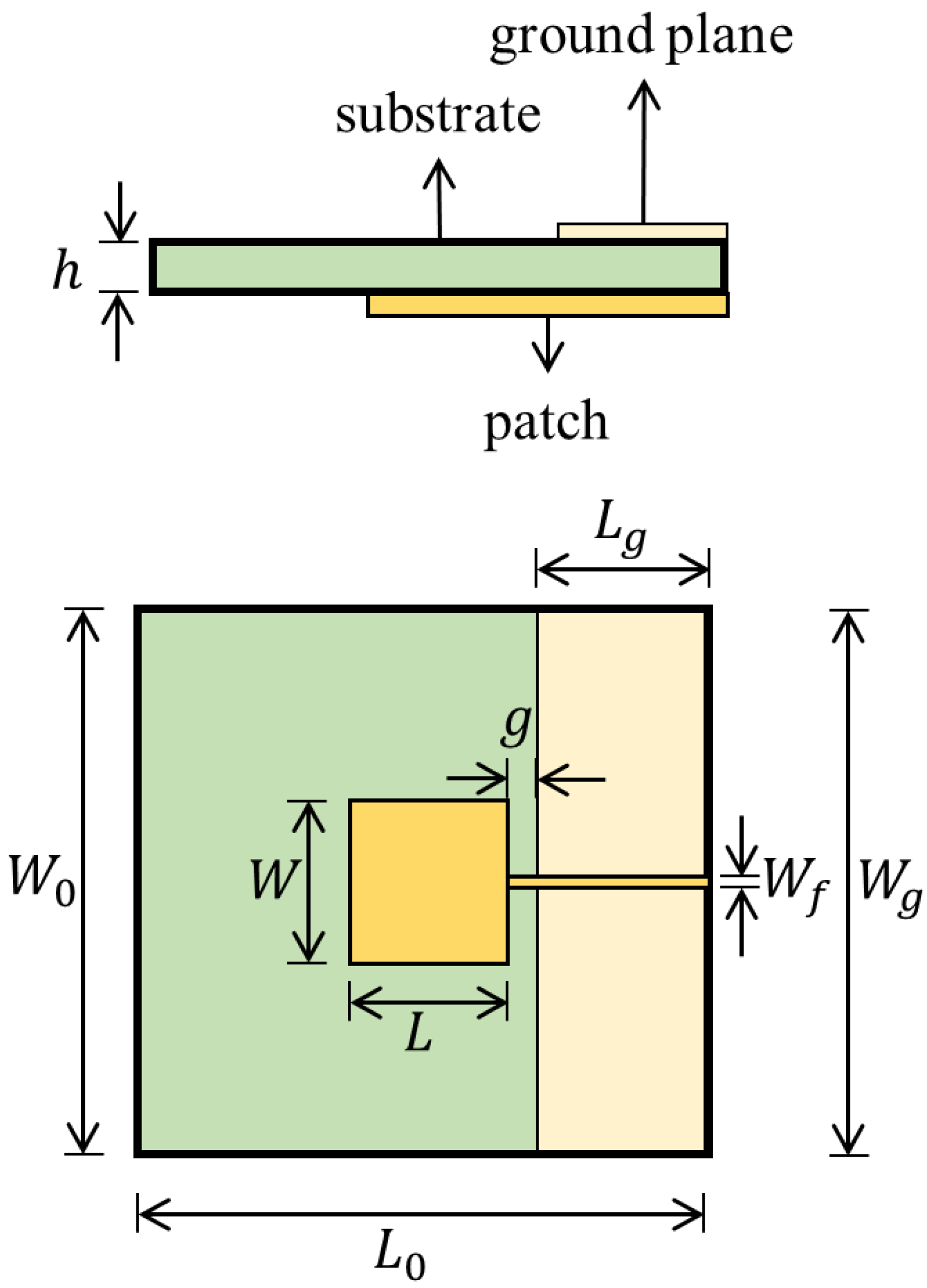
2.5.2. Planar Monopole Antenna (PMA)

PMA is an attractive option for real-world utilizations due to its cheap, omnidirectional radiation pattern, ease of installation/construction, wide bandwidth, and condensed sizes when going through the miniaturization process. They are sensitive enough to detect PD in its early stages [65,66] and can identify different signal patterns for defect classification [67]. Despite their potential, PMAs have been scarcely studied for PD localization compared to microstrip antennas [68]. The dimensions of a sample PMA are shown in Figure 4, where $L$ and $W$ are the length and width of the antenna receiving element, $L_g$ and $W_g$ are the length and width of the ground plane, $W_f$ is the signal transmission width, and $h$ is the thickness of the substrate.

The efficiency of the PMA can be improved by maximizing the receiving element perimeter. To achieve this, some bioinspired PMA designs such as leaf [69], butterfly [70], and bee [71] have been explored. An antenna inspired by Jatropha Mollissima leaf was developed in [66] for PD localization in [72]. With a −5 dB limit of reflection coefficient, it has a PD detection range from 772 to 1272 MHz, with an approximate 70% power signal transmitted. The detected PD levels were higher than 35 pC, which showed that the sensitivity is satisfactory when taking measurements in power transformers. Additionally, this sensor is protected against corrosion by using the epoxy coating while its aluminium enclosure provides increased mechanical support. This makes it compatible for use with dielectric windows, with a lifespan that matches the transformer. This design is easy to manufacture and has a low cost, with the potential to utilize other bio-inspired shapes to optimize one or more parameters. PMA can handle the problems of the directional radiation pattern, irregular narrow bandwidth, and huge size for a UHF antenna. PMA can be a good option to increase the bandwidth of the antenna [73,74] as, with the approximate patch perimeter, the operating frequency can be calculated using [72] Equation (7):

$$f\left(\mathrm{GHz}\right)=\frac{300}{p\sqrt{{\epsilon }_{ref}}}$$

(7)

where ${\epsilon }_{ref}$ is the relative permittivity of the dielectric substrate and p is the perimeter of the radiator element, and then approximated as in Equation (8):

$${\epsilon }_{ref}=\frac{\left({\epsilon }_r+1\right)}{2}+\frac{\left({\epsilon }_r-1\right)}{2}{\left(1+12\frac{h}{w_f}\right)}^{-\frac{1}{2}}$$

(8)

2.5.3. Fractal Antenna

The fractal antenna is a popular choice for creating UHF sensors that are small in size while maintaining similar impedance and radiation pattern characteristics as larger antennas. This allows them to fit within the commercially recommended area for PD diagnostics. The Hilbert fractal antenna’s contours enable the compactness of antenna design, where the length of the fractal contour depends on the antenna order. The higher the antenna order $\left(n\right)$, the larger the length of the fractal contour [54]. Figure 5 shows the different antenna representations when different orders of Hilbert antenna are used.

Several design considerations are necessary to ensure the antenna performs effectively in the right power applications. This includes the physical size consideration of the antenna which involves the side length $\left(l\right)$ and the length of each line segment $\left(d\right)$, where $d$ can be obtained by Equation (9):

$$d=\frac{1}{2^{n-1}}$$

(9)

Setting the design parameters’ purpose is to maximize the allowable area of detection, such as antenna design for PD detection in a transformer may become restricted due to the limited space available. Furthermore, the number of antenna orders becomes a consideration when the cost of antenna fabrication becomes a concern. The higher the number of orders used will result in a larger segment total length $\left(s\right)$ and reduces the value $d$, where $s$ can be obtained by Equation (10):

$$s=\left(2^{2n-1}-1\right)d$$

(10)

Consequently, the complexity and the cost of fabrication increase. Meanwhile, using a suitable number of antenna orders also guarantees that the antenna’s lowest resonant frequency value is above 300 MHz for noise elimination. PD detection adopts the 4th Hilbert fractal antenna design with bending deformation developed for UHF signal detection in GIS [75]. The fact that the physical antenna’s bandwidth is not as significantly impacted by bending is evidence that the flexible antenna has strong physical stability. At 2.3 GHz with a 350 mm antenna bend radius, the antenna’s gain magnitude and directional characteristics still satisfy the criteria of UHF PD detection.

Table 3. Antenna designs and their respective variations.

Design	Variations	Reference
Spiral	Cosine slot Archimedean spiral antenna	[64]
	Archimedean spiral antenna	[76]
	Log-periodic spiral slot antenna	[77]
	Archimedean spiral antenna	[61]
	Two-arm equiangular spiral antenna	[78]
PMA	Ultra-wideband microstrip patch antenna	[79]
	Bio-inspired by the Jatropha mollissima (Pohl) Baill leaf	[66]
	Wing-shaped ultra-wide band monopole antenna	[73]
	Bio-inspired by Inga Marginata leaf	[65]
	Ultra-Wide Band Antenna	[80]
Fractal	4th-order Hilbert antenna	[75]
	4th-order Hilbert antenna	[54]
	Moore fractal antenna	[81]
	3rd-order stacked Hilbert antenna	[82]
	4th-order Hilbert antenna	[83]

Table 3. Antenna designs and their respective variations.

Design	Variations	Reference
Spiral	Cosine slot Archimedean spiral antenna	[64]
	Archimedean spiral antenna	[76]
	Log-periodic spiral slot antenna	[77]
	Archimedean spiral antenna	[61]
	Two-arm equiangular spiral antenna	[78]
PMA	Ultra-wideband microstrip patch antenna	[79]
	Bio-inspired by the Jatropha mollissima (Pohl) Baill leaf	[66]
	Wing-shaped ultra-wide band monopole antenna	[73]
	Bio-inspired by Inga Marginata leaf	[65]
	Ultra-Wide Band Antenna	[80]
Fractal	4th-order Hilbert antenna	[75]
	4th-order Hilbert antenna	[54]
	Moore fractal antenna	[81]
	3rd-order stacked Hilbert antenna	[82]
	4th-order Hilbert antenna	[83]

3. Conventional Localization Technique

The previous section discussed the type of signals emitted during PD activities with their measurement strength and limitations for different applications. Additionally, several popular antenna designs based on EM detection and the respective design parameters were examined. In this section, different PD localizations using the conventional approach are discussed and tabulated in Table 4. During the PD event, emitted signals from the PD sources can be captured by the UHF, acoustic, or optical sensors positioned at various known positions. Many scholars have conducted widespread research on PD localization techniques using popular methods such as time difference of arrival (TDOA), angle of arrival (AOA), time of arrival (TOA), and received signal strength information (RSSI) to achieve the desired performance. Among them, TDOA-based localization is popular due to its better accuracy compared to other methods [84]. The AOA method is used for far-field sensor placement, which will reduce localization performance [52]. RSSI information-based methods have limitations when signals are contaminated with external noise signals, particularly when travelling in open space or within an air-insulated substation [52]. For PD detection and localization in a 3D space, at least four sensors are needed, while at least three sensors are required for 2D space. The arrangement of sensors also plays an important role in improving sensing capability, so different researchers have included studies on different sensor configurations [36,84]. However, the conventional techniques involve the solving of nonlinear equations to obtain the PD coordinate; hence, researchers also explored algorithms to linearize the equations [17,20,33,85]. Furthermore, an iterative algorithm such as Newton Raphson is needed to solve the equations to locate the PD source, and choosing an initial value is crucial to determine whether the algorithm can achieve local minima or global minima. The computation will be more complex and time-consuming as more sensors are used for PD measurement. Several widely used conventional techniques are described in the following sections.

3.1. Time Difference of Arrival (TDOA)

When the PD occurs, the EM and acoustic signal generated will travel and be detected by the sensors located at different locations, and, hence, the time difference of signal arrival to each of the sensors can be integrated into a geometric triangulation algorithm to obtain the PD coordinate. Using the TDOA at each sensor, a set of nonlinear equations can be constructed to obtain the PD location using Equations (11)–(14):

$$d_1=\sqrt{{\left(x-x_1\right)}^2+{\left(y-y_1\right)}^2+{\left(z-z_1\right)}^2}=c\left(T_1\right)$$

(11)

$$d_2=\sqrt{{\left(x-x_2\right)}^2+{\left(y-y_2\right)}^2+{\left(z-z_2\right)}^2}=c\left(T_1+t_{12}\right)$$

(12)

$$d_3=\sqrt{{\left(x-x_3\right)}^2+{\left(y-y_3\right)}^2+{\left(z-z_3\right)}^2}=c\left(T_1+t_{13}\right)$$

(13)

$$d_4=\sqrt{{\left(x-x_4\right)}^2+{\left(y-y_4\right)}^2+{\left(z-z_4\right)}^2}=c\left(T_1+t_{14}\right)$$

(14)

where ($x_i, y_i$) are the sensor’s coordinates and $i=1, 2, 3,\mathrm{and} 4$; $c$ is the speed of light; $T_1$ is the time of signal arriving sensor 1; $t_{1n}$ is the time reference of another sensor to sensor 1 and $n=2, 3, \mathrm{and} 4$. When there are numerous PD sources, there is a set of TDOAs among every PD source and two antennas [6,24,86]. The predicted localization error can be computed with Equation (15) [8].

$$e=\sqrt{{\left(x-x_c\right)}^2+{\left(y-y_c\right)}^2+{\left(z-z_c\right)}^2}$$

(15)

where ($x_c, y_c, z_c$) are the computed PD coordinates and $\left(x, y, x\right)$ are actual source coordinates.

In [6], a modified clustering algorithm called the 3σ- two-step clustering algorithm was used and followed by the Newton Raphson iterative to solve the localization equations for an air-insulated substation. The proposed clustering method localization performance was compared with [19,87,88], and it showed overall better performance in terms of iteration time and the number of PD sources located, and did not easily fall into local minima. The author used four omnidirectional RF antenna sensors to capture the PD signal and applied the TDOA technique for the PD dataset. The proposed algorithm achieved multiple PD localizations in both simulation and field tests with the performance of 0.21 m error for 2 PDs, 0.45 m error for 3 PDs under lab test, and 0.6–2 m error in a field test.

The performance of PD localization under the influence of transformer oil was evaluated in [40] via simulation and experimental works. Due to the thermosiphon effect, the top of the transformer tank region has a higher temperature than the lower region which subsequently influenced the acoustic wave propagation speed and increased the localization error. Hence, a correction-iterated method was used to overcome the acoustic wave TDOA error, and the performance showed more robustness in the localization than the Newton Raphson, imperial competitive algorithm, and genetic algorithm.

The PD localization in a 15.7 km transmission cable was established in [89] using dual-loop Sagnac interference-type optical fibre for PD detection. The PD detection sensitivity was studied from 110 sets of PD signal to investigate the influence of the length of the delay fibre, where delay fibre was directly related to changes in phase and optical power when PD occur, and the PD source sensitivity was the highest when delay fibre of different length was at 12.352 km. The cross-correlation function was used for finding the PD position along the cable, and the localization accuracy showed ±80 m for 6 km of cable.

An estimation filter algorithm of the extended Kalman-smooth variable structure filter (EK-SVSF) was used to find the PD location under a lab environment for the transformer [21]. With different case studies carried out, the filter enhanced the localization performance with noise-optimal nonlinear measurement, where it showed a faster convergence rate and minimum root mean square error (RMSE) when benchmarked with four other filter techniques, which are EKF, UKF, smooth variable structure filter (SVSF), and unscented Kalman-smooth variable structure filter (UK-SVSF). Hence, the filter has exhibited immunity to modelling uncertainties, while others’ performances were reduced.

In [24], the captured signals by UHF probes were preprocessed by the time window contrast function (TWCF) technique which acts as a window shifting method, scanning through the captured signal and calculating the mean values of each window at different samplings; hence, the new signal sets were generated which carry the signals’ arrival time (AT) sequences. The PD source localization was accomplished by considering the signal sets from both denoised and not denoised, and in the case of multiple PD occurrences, the fuzzy C-mean clustering method was used to create the clusters. However, even with the preprocessed data, the localization error complied in the range of 10 cm, and the accuracy was influenced by signal distortion and attenuation when the PD source was in a metal barrier.

The influence of varying noise distributions from different noise sources on PD localization error was studied in [1] involving the noise from the system’s model and sensors’ measurement. The maximum likelihood estimation and extended Kalman filter (EKF) were used for identifying the true noise statistics and to estimate the PD location, respectively. Placing an obstacle in front of the sensor was established to evaluate the change of time arrival error from the PD source to sensors, and the performance of EKF-MLE was better than the standalone EKF method.

A noniterative PD localization method-based TDOA was constructed in [8] for the transformer. The obtained TDOA calculation was refined by performing recurrence quantification analysis (RQA) on the cross-recurrent plot (CRP) matrix with the self-similarity parameter to reduce the TDOA calculation error which may introduce a large error influence in the source location. The algorithm was verified through the localization performance in the lab environment and showed better TDOA estimation compared to CRP using cross-correlation even under lower SNR.

3.2. Angle of Arrival (AOA)

AOA estimation on the PD source location had been widely established from the multiple signal classification (MUSIC) approaches. High-resolution AOA estimation can be obtained using the orthogonality between the noise subspace and the signal subspace, and it showed better efficiency than the maximum likelihood estimation (MLE) approach under a low SNR status. The flowchart in Figure 6 shows the MUSIC algorithm processes.

An enhanced particle swarm optimization (PSO) algorithm was applied in [3] on the 3D localization for substation application. An antenna array which consists of two UHF sensors was used to take the measurement for DOA and followed by TDOA. PSO was first used to optimize the 2D (x and y axis) before proceeding to optimize the height (z-axis), which is the distance between the sensors’ array and the PD source. The algorithm avoids falling into the local optimal with the equation with the highest weight in the plane coordinates. The suggested algorithm showed greater performance for the localization error and time taken to complete the localization calculation as compared to [32,90,91,92].

A work in [18] used the N × N sensor array with N < 5 to locate (N − 1) number of PD sources. The effort of compressive sensing (CS), MUSIC algorithm, and peak search were involved by virtually extending the 2 × 2 UHF sensor array to a higher dimension array, constructing the PD source spatial spectrum and locating the PD directional angle, respectively. Both simulations and experiments were conducted, and the localization performance improved when the sensor array increased; however, the estimation error increased significantly when the sensor array extended to 5 × 5. The algorithm has the strength to identify and locate multiple PD sources with great accuracy, but it needs more sensors and a larger array size for cultivation.

3.3. Time Reversal (TR)

The time reversal technique uses time reversal invariance to diverge the transmitted signal back to its emitting source to locate the source [25]. PD source localization using the TR technique can be applied to acoustic (ATR) or electromagnetic (EMTR) signals and the processes of TR are summarized below [23,86]:

• During the forward time step, PD signals are emitted from one or multiple sources at a distance and captured by single or multiple sensors.
• The captured signal undergoes time reversing.
• The time-reversed signal is back injected into the medium in the backpropagation step.
• The criterion algorithm such as maximum field, minimum entropy, or cross-correlation [25] can be applied to locate the focal spot created by constructive interference to locate the PD coordinate, based on the notion that the waves will refocus at the primary source site both in time and space.

In [23], a time reversal (TR) technique was used to localize the PD source in the transformer in 3-dimensions using a single acoustic sensor located outside of the transformer tank. The localizations were simulated in MATLAB toolbox (k-Wave), and different scenarios were tested to show the performance of the proposed method including PD source(s) inside the transformer winding, in between the windings, two simultaneous PD sources, and between a vertical branch and a coil of the magnetic circuit. The performance showed accurate localization in the normalized pressure figures. The first two cases showed better performance as compared to the simulation from [22] which used 2D simulations. The reason is that 3D provided more paths between the PD source and the acoustic sensor as compared to 2D.

A 3D simulation for PD localization in a transformer using the acoustic time reversal (ATR) method was presented in [86] using an individual acoustic sensor. The 3D numerical model of the transformer was evaluated using the finite element method (FEM) which aims to analyse the acoustic wave propagation in the transformer. Seventeen different case studies were carried out to assess the ATR performance including against the TDOA technique to locate multiple real PD sources in a lab environment. The ATR method performed better than the TDOA in all the studies.

A 2D simulation in a transformer for PD source localization was carried out using the time reversal (TR) technique [22] with one sensor. A combination of a 2D finite-difference time domain (FDTD) and a minimum entropy criterion (MEC) was used to investigate how acoustic waves propagate and determine the focal spot to identify the PD location, respectively. Different scenarios were simulated such as PD source within the transformer windings and between two transformer windings, and the localization accuracies showed accurate PD location which was presented in a normalized distribution plot.

The electromagnetic time reversal (EMTR) technique was applied to identify the PD source location in the transformer under both simulation and lab environments [25]. The 2D finite-difference time domain (FDTD) was used to evaluate the electric field inside the transformer tank in the backward and forward time steps when different PD source locations were studied, and the maximum field criterion (MFC) was applied for obtaining the PD coordinates. The performance of EMTR with a single sensor was compared with the TDOA method with three sensors; the EMTR method showed better results when the PD source in between the transformer windings was involved.

The electromagnetic time reversal (EMTR) PD source localization was accomplished in [93] for a 33 kV power line in between the two substations without the need for any denoising algorithm. The 1D transmission line matrix (TLM) model was used to describe the PD signals’ propagation in the reversed time, and the PD source location can be identified from the guessed PD locations (GPDLs) with the highest energy concentration. Different levels of SNR noises were artificially added into the PD signal, and the algorithm achieved 0.5% of error for an SNR of −7 dB using lesser computational time. In contrast, for the method to work properly, the line length and the PD signal propagation speed must be known.

3.4. Received Signal Strength Index (RSSI)

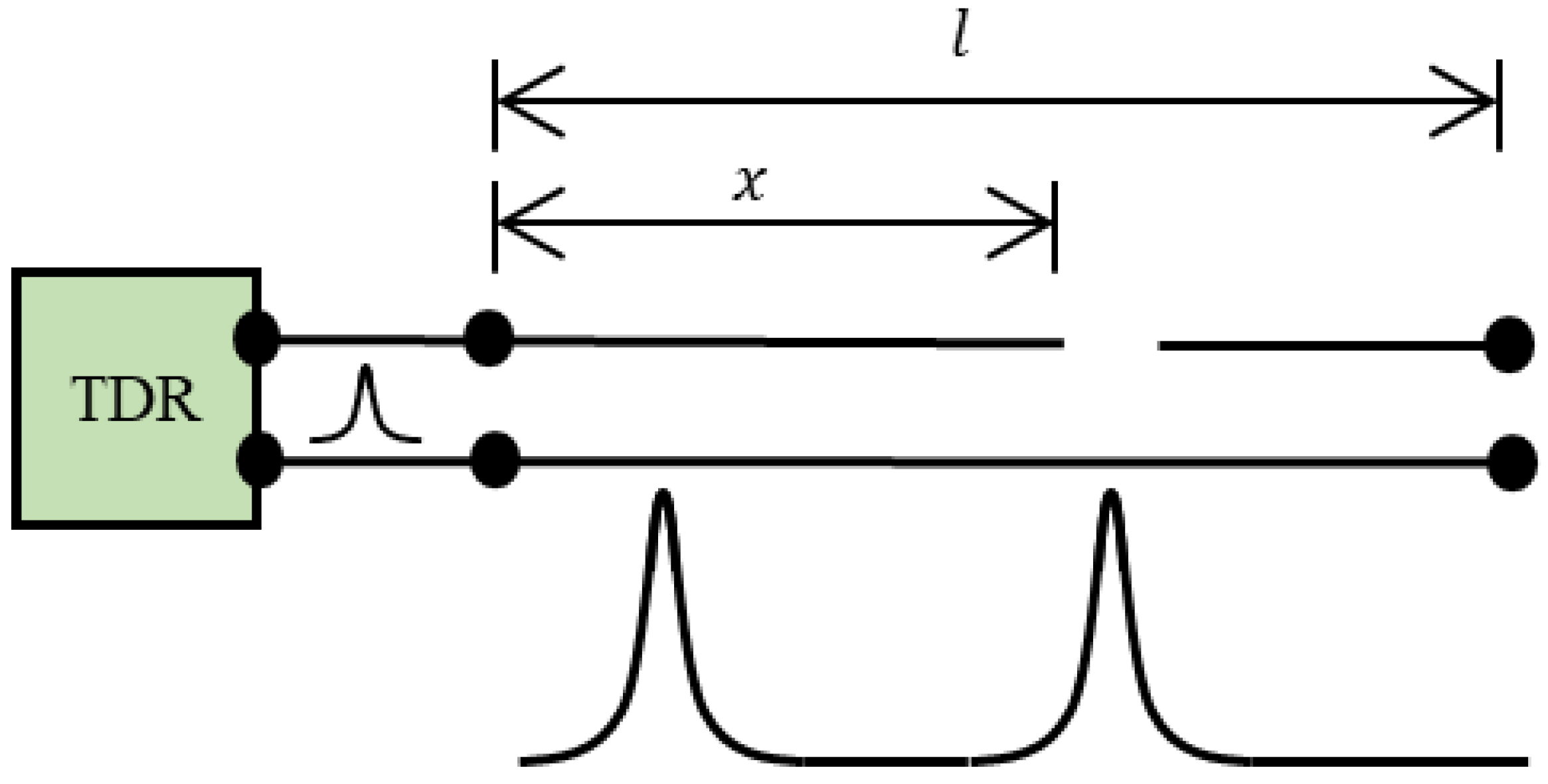
The benefits of using the RSSI technique over TDOA or AOA are due to its simplicity in hardware requirements, it being less expensive [94], and its suitability for large-scale deployment [16]. The RSSI technique can be implemented using two different approaches: the transmission model and the fingerprint map approach. The transmission model approach utilizes the RSSI information to acquire the signal transmission loss between the known and unknown position before transforming it into a distance according to the model [16]. The RSSI value of transmission can be expressed as in Equation (16):

$$RSSI\left(d\right)=RSSI\left(d_0\right)-10n.log\left(d\right)+X_{\sigma }$$

(16)

where $d_0$: reference distance; $n$: attenuation factor; and $X_{\sigma }$: Gaussian random variable. Ignoring the Gaussian random variable, the RSSI value at distance $d$ can be expressed in Equation (17):

$$RSSI\left(d\right)=A-10n.log\left(d\right)$$

(17)

where $A=RSSI\left(d_0\right)$ with the reference signal is 1 m.

In the fingerprint map approach, the PD localization processes involve both the offline and online stages. During the initial offline stage, the PD will be simulated multiple times in a specified test zone to obtain sufficient fingerprint data from the captured RSSI value by the sensor. The fingerprint information collected is used to train the machine learning model for future PD location recognition. When PD occurred during the online stage, the trained model was able to identify the PD location using the measured RSSI value. The fingerprinting approach is more reliable compared to the transmission model approach because it works effectively under a complex spatial environment.

3.5. Reflectometry

The fundamental principle of reflectometry is to inject a low-voltage pulse (reference signal) into the test cable; the reflection signal generated can be calculated to indicate the point of reflection. By measuring the difference in time between the reference signal and the reflected signal, and knowing the propagation velocity of the pulse, the reflection point can be identified. The reflection point is the impedance discontinuity point and is where PD activities occur or is open-ended cable [95]. The time-domain reflectometry (TDR) technique is the most established and widely used measuring technique for the identification of cable impedance discontinuity. The distance of fault from the signal-injecting-end as shown in Figure 7 can be calculated by Equation (18):

$$x=l-v\frac{t_2-t_1}{2}$$

(18)

where $v=\frac{c}{\sqrt{{\in }_r}}; l$: cable length; $t_1$: time taken of signal travel from defect point to signal-injecting-end; $t_2$: time taken of signal travel from defect point to cable end and to signal-injecting-end; $v$: wave propagation speed; $c:3\times {10}^8 \mathrm{m}/\mathrm{s}$; and ${\in }_r$: relative permittivity of the dielectric [96].

In [96], multiple PD sources in the cable were distinguished by using the spectral power ratio (PR) which separated the signal into higher and lower frequency bands. PSO was used to further distinguish the PD sources by increasing the cluster centroid distance of each PD source. The PD source location was found by determining the relative propagation between the incident and reflected pulses which is known as TDR. By computing the time difference of arrival (TDOA) of the incident and reflected pulse, the PD location was found with a worst error of 5%.

3.6. Others

Researchers in [42] used the energy distribution from mathematical morphology (MM) to locate two different types of PD sources simultaneously at the transformer terminals. The denoising and clustering technique known as hard-thresholding and ordering points to identify clustering structure (OPTICS) was used for noise reduction and PD source separation, and the location was determined based on the energy contained in both of the sensing points which are located at the bushing and neutral measurement points. However, it only provided the indication either near the bushing tap-point or near the neutral-to-earth tap-point or at the centre of both, which does not indicate which terminal is the origin of the PD.

In [97], PD source localization using the lumped parameter ladder network model was used to locate PD up to the disc-to-disc level of the transformer. The location of the PD was identified by having a maximum correlation value between the reference and test signals. The reference signal was obtained from the simulation on the ladder network model while the test signals were acquired by exciting the laboratory winding with PDs of 5 pC to 5000 pC using a PD calibration kit. However, the localization focuses on identifying the PD source at the predefined section of the winding turns. The PD source identification and localization were established using the pulse compression technique and linear frequency modulation (LFM) [95]. The combination of algorithms provided the optimization between detection distance and high localization accuracy by improving the fault detection resolution from the reflected signal in the leaky coaxial cable (LCX). The algorithm performance was evaluated and compared in a lab environment with the TDR technique, and it had the lowest error at the furthest distance of 130 m.

There are other reports in [44] using a noniterative algorithm which can show satisfactory results using lesser computational power and time. The combined acoustic–electrical detection used the signal absolute time instead of time arrival for the PD location measurements, and the performance was compared with the noniterative method using four acoustic sensors (time difference approach) and the Newton Raphson iterative method. The algorithm showed the ability to locate the PD source accurately. However, the performance of the algorithm may be affected by electrical noise and the influence of varying transformer insulating oil temperatures.

Table 4. Conventional PD localization.

Ref.	Application	Type of Sensors	Method (Algorithm)	Proposed Method Outperforms the Following Algorithm	Simulation/ Experimental	Performance
[23]	Transformer	1 Acoustic sensor (TR)	ATR (3D)	ATR (2D)	Simulation	Correctly identified in a simulated 0.4 × 1 × 0.4 m space
[86]	Transformer	1 Acoustic Sensor (TR)	ATR	TDOA	Both	Correctly identified PD in the presence of noise
[39]	Transformer	4 Acoustic sensors (TDOA)	Singular spectrum analysis-independent component analysis (SSA-ICA) with cumulative energy function	Customed SSA Ensemble empirical mode decomposition-independent component analysis (EEMD-ICA)	Both	Lowest error of 132.20 mm
[98]	Transformer	8 fibre-optic acoustic sensors (TDOA)	Levenberg–Marquardt algorithm using FEM simulation results	No comparison performed	Simulation	5 cm error
[40]	Transformer	4 Acoustic sensors (TDOA)	Correction-Iterative Method	Newton’s method Genetic algorithm (GA) Imperial competitive algorithm (ICA)	Both	Maximum error: 49.97 mm
[99]	Transformer	lattice-rogowski-coil sensor	Measuring and identify the highest voltage value among different location in transformer as the PD	No comparison performed	Experimental	Maximum peak value of voltage showed the closest distance from sensor to PD source
[85]	Transformer	5 Acoustic sensors (TDOA)	Optimized L-TSVD	Direct TSVD method Newton iteration method	Experimental	15.52 cm error
[41]	Transformer	4 UHF sensors (TDOA)	CHAN algorithm	No comparison performed	Both	15 cm error
[43]	Transformer	8 Ultrasonic sensors (TDOA)	Semidefinite Relaxation Convex Optimization	CHAN PSO	Both	Localization error of 0.1 m
[42]	Transformer	2 RFCTs	OPTICS + MM	No comparison performed	Experimental	The $R_D$ values able to identify the near or far between sensor and PD source
[21]	Transformer	1 RF antenna + 3 Acoustic sensors (TDOA)	EK-SVSF	Extended Kalman filter (EKF) Unscented Kalman filter (UKF) Smooth variable structure filter (SVSF) UK-SVSF	Experimental	EK-SVSF achieved faster convergence and lower RMSE than others
[25]	Transformer	1 sensor (TR)	2D-FDTD + MFC	TDOA	Both	Localization error of 10 mm (corresponding to λ_min/10)
[22]	Transformer	2 Acoustic sensors (TR)	2D-FDTD + MEC	No comparison performed	Simulation	Accurately located PD in a simulated 0.4 × 1 m dimension
[24]	Transformer	4 UHF probes (TDOA)	Time Window Contrast Function (TWCF)	Average time window threshold (ATWT) Modified Dynamic cumulative sum (DCS)	Experimental	Error in the range of 10 cm
[44]	Transformer	3 Acoustic + 1 Electrical sensors	Noniterative acoustic-electrical	Newton iterative method Non-iterative method (used in all-acoustic system with 4 sensors—time-difference approach)	Experimental	$\mathrm{Correctly}\mathrm{identified}\mathrm{the}\mathrm{PD}\mathrm{with}\mathrm{less}\mathrm{than}2.23\times {10}^{-4}$ computational time
[8]	Transformer	4 UHF sensors (TDOA)	CRP based Self-Similarity-RQA of non-iterative method	Cross-correlation-CRP	Both	Efficient TDOA estimation under low SNR
[97]	Transformer	PD detector	Ladder Network Model	No comparison performed	Both	Accurately located PD from the maximum correlation
[1]	Transformer	3 Acoustic sensors (TDOA)	EKF-MLE	EKF	Experimental	MLE-EKF performed better in the presence of barrier in front of sensor
[3]	Substation	2 UHF sensors (DOA + TDOA)	Improved PSO	Direct PSO Iterative grid search solution Spatial grid search Error Probability Distribution- localization	Experimental	0.21 m error
[6]	Substation	4 UHF sensors (TDOA)	3σ-Two Step algorithm	PSO Hybrid DE-PSO Probability-based combine K-means RSSI	Experimental	Lab test: 0.21 m error for 2 PDs 0.45 m error for 3 PDs Field test: 0.6–2 m error
[19]	Substation	3 UHF sensors (AOA + RSSI)	MUSIC	AOA + RSSI without MUSIC	Experimental	error less than 1 degree
[32]	Substation	4 UHF sensors (TDOA)	generalized S-transform (GST) + Newton Iterative	Without denoising WT (db2) WT (db8)	Both	Errors in 3D and 2D are 1.59 m and 0.11 m respectively
[20]	Substation	5 UHF Antennas (TDOA)	Tikhonov Regularization Method (with centralization and row balance)	Gaussian elimination direct regularization method	Both	Simulation: 2.99 m error Experiment: 2.33 m error
[33]	Substation	5 UHF sensors (TDOA)	Truncated singular value decomposition (TSVD) Regularization with generalized cross-validation (GCV)	Gaussian elimination method direct TSVD regularization method Tikhonov regularization method	Both	Simulation: 2.02 m error Experimental: 2.07 m error
[18]	Substation	N × N UHF sensor array; 1 < N < 5 (DOA)	CS + MUSIC + Peak Search	No comparison performed	Both	Error reduced from 12 degree to 4 degree
[93]	Cable	1 HFCT (TR)	EMTR-1D TLM	No comparison performed	Both	Without/With noise: 0.14%/0.5% error
[100]	Cable	- (EMTR)	TLM	No comparison performed	Simulation	Error < 1.5%
[89]	Cable	2 Photodetector (TDOA)	Cross-Correlation	No comparison performed	Experimental	±80 m for 6 km cable
[96]	Cable	1 HFCT (TDR)	Power Ratio (PR) with PSO + TDR	No comparison performed	Experimental	Maximum of 5% error
[95]	Cable	-	Linear frequency modulation (LFM) + Pulse Compression technique	TDR	Experimental	LFM: error from 0.09–1.43 m TDR: error from 0.48–4.77 m

Table 4. Conventional PD localization.

Ref.	Application	Type of Sensors	Method (Algorithm)	Proposed Method Outperforms the Following Algorithm	Simulation/ Experimental	Performance
[23]	Transformer	1 Acoustic sensor (TR)	ATR (3D)	ATR (2D)	Simulation	Correctly identified in a simulated 0.4 × 1 × 0.4 m space
[86]	Transformer	1 Acoustic Sensor (TR)	ATR	TDOA	Both	Correctly identified PD in the presence of noise
[39]	Transformer	4 Acoustic sensors (TDOA)	Singular spectrum analysis-independent component analysis (SSA-ICA) with cumulative energy function	Customed SSA Ensemble empirical mode decomposition-independent component analysis (EEMD-ICA)	Both	Lowest error of 132.20 mm
[98]	Transformer	8 fibre-optic acoustic sensors (TDOA)	Levenberg–Marquardt algorithm using FEM simulation results	No comparison performed	Simulation	5 cm error
[40]	Transformer	4 Acoustic sensors (TDOA)	Correction-Iterative Method	Newton’s method Genetic algorithm (GA) Imperial competitive algorithm (ICA)	Both	Maximum error: 49.97 mm
[99]	Transformer	lattice-rogowski-coil sensor	Measuring and identify the highest voltage value among different location in transformer as the PD	No comparison performed	Experimental	Maximum peak value of voltage showed the closest distance from sensor to PD source
[85]	Transformer	5 Acoustic sensors (TDOA)	Optimized L-TSVD	Direct TSVD method Newton iteration method	Experimental	15.52 cm error
[41]	Transformer	4 UHF sensors (TDOA)	CHAN algorithm	No comparison performed	Both	15 cm error
[43]	Transformer	8 Ultrasonic sensors (TDOA)	Semidefinite Relaxation Convex Optimization	CHAN PSO	Both	Localization error of 0.1 m
[42]	Transformer	2 RFCTs	OPTICS + MM	No comparison performed	Experimental	The $R_D$ values able to identify the near or far between sensor and PD source
[21]	Transformer	1 RF antenna + 3 Acoustic sensors (TDOA)	EK-SVSF	Extended Kalman filter (EKF) Unscented Kalman filter (UKF) Smooth variable structure filter (SVSF) UK-SVSF	Experimental	EK-SVSF achieved faster convergence and lower RMSE than others
[25]	Transformer	1 sensor (TR)	2D-FDTD + MFC	TDOA	Both	Localization error of 10 mm (corresponding to λ_min/10)
[22]	Transformer	2 Acoustic sensors (TR)	2D-FDTD + MEC	No comparison performed	Simulation	Accurately located PD in a simulated 0.4 × 1 m dimension
[24]	Transformer	4 UHF probes (TDOA)	Time Window Contrast Function (TWCF)	Average time window threshold (ATWT) Modified Dynamic cumulative sum (DCS)	Experimental	Error in the range of 10 cm
[44]	Transformer	3 Acoustic + 1 Electrical sensors	Noniterative acoustic-electrical	Newton iterative method Non-iterative method (used in all-acoustic system with 4 sensors—time-difference approach)	Experimental	$\mathrm{Correctly}\mathrm{identified}\mathrm{the}\mathrm{PD}\mathrm{with}\mathrm{less}\mathrm{than}2.23\times {10}^{-4}$ computational time
[8]	Transformer	4 UHF sensors (TDOA)	CRP based Self-Similarity-RQA of non-iterative method	Cross-correlation-CRP	Both	Efficient TDOA estimation under low SNR
[97]	Transformer	PD detector	Ladder Network Model	No comparison performed	Both	Accurately located PD from the maximum correlation
[1]	Transformer	3 Acoustic sensors (TDOA)	EKF-MLE	EKF	Experimental	MLE-EKF performed better in the presence of barrier in front of sensor
[3]	Substation	2 UHF sensors (DOA + TDOA)	Improved PSO	Direct PSO Iterative grid search solution Spatial grid search Error Probability Distribution- localization	Experimental	0.21 m error
[6]	Substation	4 UHF sensors (TDOA)	3σ-Two Step algorithm	PSO Hybrid DE-PSO Probability-based combine K-means RSSI	Experimental	Lab test: 0.21 m error for 2 PDs 0.45 m error for 3 PDs Field test: 0.6–2 m error
[19]	Substation	3 UHF sensors (AOA + RSSI)	MUSIC	AOA + RSSI without MUSIC	Experimental	error less than 1 degree
[32]	Substation	4 UHF sensors (TDOA)	generalized S-transform (GST) + Newton Iterative	Without denoising WT (db2) WT (db8)	Both	Errors in 3D and 2D are 1.59 m and 0.11 m respectively
[20]	Substation	5 UHF Antennas (TDOA)	Tikhonov Regularization Method (with centralization and row balance)	Gaussian elimination direct regularization method	Both	Simulation: 2.99 m error Experiment: 2.33 m error
[33]	Substation	5 UHF sensors (TDOA)	Truncated singular value decomposition (TSVD) Regularization with generalized cross-validation (GCV)	Gaussian elimination method direct TSVD regularization method Tikhonov regularization method	Both	Simulation: 2.02 m error Experimental: 2.07 m error
[18]	Substation	N × N UHF sensor array; 1 < N < 5 (DOA)	CS + MUSIC + Peak Search	No comparison performed	Both	Error reduced from 12 degree to 4 degree
[93]	Cable	1 HFCT (TR)	EMTR-1D TLM	No comparison performed	Both	Without/With noise: 0.14%/0.5% error
[100]	Cable	- (EMTR)	TLM	No comparison performed	Simulation	Error < 1.5%
[89]	Cable	2 Photodetector (TDOA)	Cross-Correlation	No comparison performed	Experimental	±80 m for 6 km cable
[96]	Cable	1 HFCT (TDR)	Power Ratio (PR) with PSO + TDR	No comparison performed	Experimental	Maximum of 5% error
[95]	Cable	-	Linear frequency modulation (LFM) + Pulse Compression technique	TDR	Experimental	LFM: error from 0.09–1.43 m TDR: error from 0.48–4.77 m

4. Machine Learning Localization

The previous section summarized the conventional localization techniques. On the other hand, there is an emerging trend of using ML in PD diagnosis to automate complex tasks and increase the accuracy of predictions. ML approaches can reduce the tendency to get stuck in local minima and avoid computation-intensive iterative calculations. The benefits of machine learning include better decision-making, enhanced efficiency, and cost savings. In this section, several popular machine-learning models used for PD diagnostics are discussed and tabulated in Table 5.

4.1. Fuzzy Logic (FL)

Fuzzy logic is a computing technique of fuzzy logic theory in which the decision is made based on “how likely it will happen” rather than from the Boolean logic (0 or 1), and the mapping of input to the output space is nonlinear. The fuzzy logic to locate the PD can be categorized into three steps [30,45]:

• Fuzzification: convert the crisp input set into a fuzzy set using the predefined membership function.
• Inference: apply the antecedent (IF) and consequent (THEN) rules using different fuzzy operators onto the “If” condition.
• Defuzzification: the output value (PD location) can be obtained.

In [45], the technique of TOA-first peak with the combination of fuzzy logic Takagi–Sugeno (FLTS) was used for the PD source(s) localization in transformer oil. The acoustic emission sensors followed by a preamplifier gain unit were used to capture the PD source at two different locations in the transformer separately. The signals were preprocessed using discrete wavelet transform (DWT) for denoising. The processed signals were further analysed and compared among different localization techniques including TOA, fuzzy logic Mamdani (FLM), and FLTS. FLTS showed better results compared to FLM and TOA by having the lowest percentages of differences in the two separate PD locations. This is because the mixture of crisp function and firing strength in FLTS can simplify the best two locations’ classes, where overall accuracy is between 96% and 97% for the two locations.

In [49], the adaptive neuro-fuzzy inference system (ANFIS) accompanied by virtual sensors (VS) and an optical simulation fingerprint were used for predicting the detection values for the sensors in PD source localization in gas-insulated transmission lines (GIL). The optical simulation localization was based on [101] which used four actual sensors (AS) and five simulated VS to generate the optical PD detection fingerprint. The sensors at the nine locations were simulated in the same GIL model, which solves the difficulty of fingerprint collection in actual equipment. The ANFIS greatly reduces the amount of AS while maintaining the desired localization accuracy. The localization error showed lower values as compared with UHF, optical, and acoustic, and further showed superior localization in the z-axis direction, which indicates it satisfied the fault location of equipment with long axial lengths such as GIL.

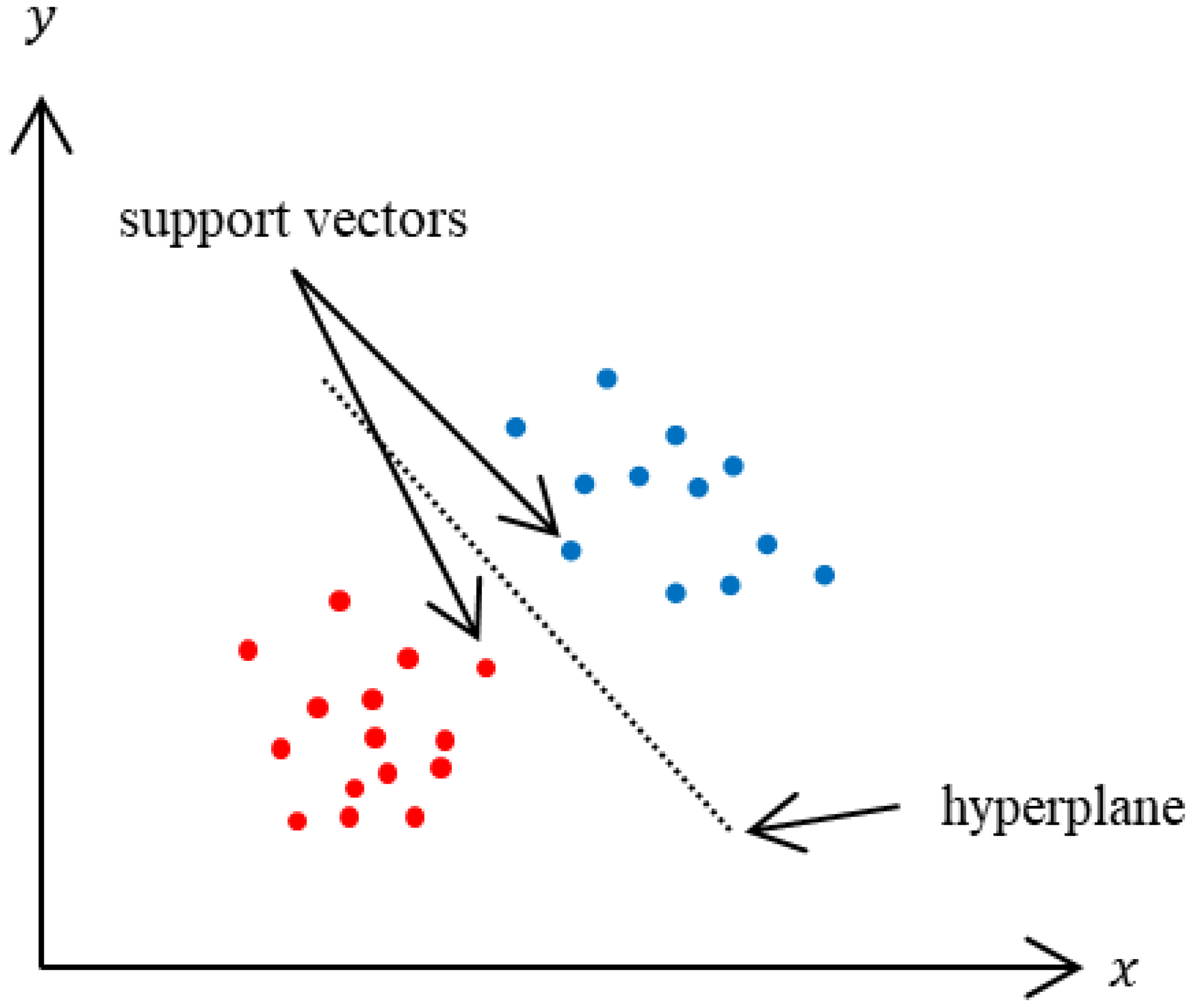
4.2. Support Vector Machine (SVM)

SVM is a supervised machine learning technique used in classification problems. The classification can be done by obtaining the hyperplane that differentiates between the two distinct classes, and by maximizing the margin distance between the classes’ data points, the accuracy can be improved when dealing with new test data. Figure 8 illustrates the classification between two different classes using SVM.

The loss function that aids in maximizing the margin between the data points and the hyperplane is called hinge loss. If the projected value and the actual value have the same sign, then the cost is zero. Otherwise, the loss value can be obtained from Equation (19):

$$c\left(x,y,f\left(x\right)\right)=\{\begin{array}{c}0,\hspace{1em}\hspace{1em}\hspace{1em}if y\times f\left(x\right)\ge 1\\ 1-y\times f\left(x\right),\hspace{1em}\hspace{1em}\hspace{1em}\hspace{1em}else\end{array}$$

(19)

The feasibility of a real-time PD monitoring system was investigated in [102] with the utilization of the ML technique. A low-cost wireless sensor network (WSN) was used to autonomously and continually build the spatial RSS map itself in the lab test environment to simulate the substation. Four different ML algorithms were used and compared [103,104,105,106] where the least-square support vector regression (LSSVR) outperformed the rest with an error of less than 2 m.

The S-Transform and random forest (RF) algorithms were used in [29] for detecting single and multiple PD sources in a simulated transformer under a lab environment using optical sensors. Sixteen features were extracted using the S-Transform from a single PD source. Several simulations were conducted using recursive feature elimination to investigate how the PD localization performance is affected by different numbers of features used. The important features selected were used to train the random forest classifier to predict the PD source coordinates, where the simulated 5, 10, and 15 features showed an accuracy of 95.6%, 98.2%, and 100%, respectively. The RF algorithm accuracy was compared and showed superiority over three other algorithms [107,108,109]. However, the results did not show a clear performance comparison of single and multiple PD sources.

Locating the PD source in the GIS bus bar is presented in [28] with a lesser number of sensors, hence, avoiding the need for high sampling synchronization. The use of the Canny algorithm involved feature extraction by detecting the ranges of edges in images to locate the PD in the longitudinal location (TDOA), while SVM as a classifier was trained to determine the circumferential position of the PD source (AOA). The proposed method achieved PD circumferential localization accuracy of 100%.

4.3. Ensemble Model—Decision Tree (DT) and Random Forest (RF)

A decision tree is a nonparametric supervised learning algorithm and is widely used in classification and regression applications. It has a hierarchical tree structure, which consists of a root node, branches, internal nodes, and leaf nodes. The decision making can be achieved by establishing the attribute and category relationship in the flowchart-like structure. PD classification using a decision tree is illustrated in Figure 9.

While decision trees are typically supervised learning algorithms, they have a tendency for overfitting and bias. Hence, the random forest algorithm with the ensemble of multiple decision trees can predict more accurate results, particularly when the individual trees are uncorrelated from each other. Each tree in the random forest separates a class prediction and the class with the greatest votes ends up being the model’s final output.

The ML ensemble of regression random forest (RRF) for a single PD source localization was implemented in [27] for the substation. The signals captured in the lab environment by the omnidirectional antennas were preprocessed using wavelet packet transform (WPT) and principal component analysis (PCA) to separate the signal and the noise based on the extracted features, which is an important step to facilitate the ML learning process and generalization steps for a better localization performance. During testing, RRF outperformed the regression tree and bootstrap aggregating algorithms.

4.4. Others

The probability grid search (PGS) was used in [52] for reducing the negative influence on the estimated TDOA values and improving the PD localization performance in a medium-sized distribution substation. The captured PD signals were first fed into a 10th order infinite impulse response (IIR) bandpass filter to remove unwanted noises. Additionally, a clustering algorithm known as a self-organizing feature map (SOFM) was used to group the data into four clusters of TDOA sets based on the four UHF sensors used. The physical layout of the test area needs to be known to allow the algorithm to perform at its best, and hence, the localization errors will decrease when the number of points, i.e., grids within the specified test areas, increases. The algorithm was shown to have better performance than active search (AS) without nearest neighbour (NN) and AS with NN in both lab and field tests.

The unsupervised classifier of the self-organizing feature map (SOFM) for detecting the number of PD sources without training data and the cross-correlation (CC) method for PD localization was used in [34] at a substation. The collected TDOA data from the UHF sensors were analysed by continuous wavelet transform and extracted into a feature matrix before presenting into SOFM for the number of PD detections. The multiple PD recognition and localization error performance showed satisfying results in both lab and field tests. However, there is a lack of localization algorithms used for the performance comparison.

A low-cost PD localization technique using purely RF-received signal features was used in [110]. The PD localization performance using the RF-received signal features was better in K-nearest neighbour with correlation-based feature selection (KNN-CFS) than in KNN without CFS. The CFS acts as a feature selector for choosing the important feature parameters and avoiding computational complexity with dimension reduction for improved accuracy. The ML algorithm KNN with CFS for localization evaluation which employs the significant features rather than directly using the uncorrelated PD features can avoid having a larger data size by reducing the feature space by 80% while improving the accuracy.

A novel PD source localization algorithm utilized the strength of large fingerprint mapping in back propagation (BP) to offset the limitation of compressed sensing (CS) presented in [35] where it can overcome the influence of the complex substation environment. For the preliminary localization, the BP was trained in the offline stage to establish a small RSSI fingerprint map, and PSO was adopted to improve the initial weight selection of the BP before the actual localization was conducted in the online stage because the RSSI intensity will be different in both stages. For the actual localization in the online stage, the CS algorithm was used to obtain more accurate results, and it shows a better performance than just using PSO-BP and BP alone. The fingerprint map requires revision from time to time because the UHF signal will be sensitive to the detection area, and it may become a time-consuming process. Hence, a reconstruction algorithm based on CS theory was used to rebuild the fingerprint map by using only a subset of the original fingerprint data.

Table 5. ML PD localization.

Ref.	Application	Type of Sensors	Method (Algorithm)	Proposed Method Outperforms the Following Algorithm	Simulation/ Experimental	Performance
[52]	Substation	4 UHF sensors (TDOA)	PGS	Active Search with Nearest-Neighbour (NN) Active Search without Nearest-Neighbour (NN)	Both	Laboratory errors: Active-Set without NN: 5.98% Active-Set with NN: 3.83% Probabilistic Grid-Search: 2.12%
[110]	Substation	3 RF monopole antenna	CFS + KNN	KNN without CFS	Experimental	Error reduced by 36.54%
[27]	Substation	3 UHF sensors	WPT + RRF	Regression tree algorithm Bootstrap aggregating method	Experimental	91% accuracy within 0.31–3.0 m error
[34]	Substation	4 UHF sensors (TDOA)	SOFM + CC	No comparison performed	Experimental	Multiple PD detection lab: average 94.9% field: average 91.6% Localization error lab: 1.3% field: 1.33%
[102]	Substation	3 omnidirectional antennas (RSS)	LSSVR	Multilayer perceptron (MLP) Radial basis function (RBF) neural network	Experimental	Error less than 2 m
[35]	Substation	4 UHF sensors (RSS)	PSO-BP + CS	PSO-BP BP	Experimental	0.89 m and 90.4% localization errors are less than 2 m
[45]	Transformer	3 Acoustic Sensors (TOA)	FLTS	TOA Fuzzy logic Mamdani (FLM)	Experimental	Accuracy is between 96% and 97% for locations 2 and 1
[17]	Transformer	8 Acoustic Sensors (TDOA)	AFC-DPC	Simulation: Density-Based Spatial Clustering of Applications with Noise (DBSCAN) K-Means DPC Experimental: Newton-Raphson CHAN GA ICA	Both	Simulation error 1.7 cm Experimental error 5.30 cm
[29]	Transformer	5 Optical sensors	S-Transform + Random Forest	Inductive inference algorithm Wavelet Transform Rough Set theory	Both	5 features: 95.6% 10 features: 98.2%. 15 features: 100%
[26]	GIL	9 Optical sensors	Bagging—kernel extreme learning machine (KELM)	Traditional KELM Back propagation neural network (BPNN)	Both	Error of 0.93 cm
[49]	GIL	4 Actual Sensors + 5 Virtual Sensors	ANFIS	UHF Optical Acoustic	Both	~Error reduced by 54.8% by adding virtual sensors with localization error of 19.69 mm
[28]	GIS	2 UHF sensors (TDOA + AOA)	Canny algorithm + SVM	No comparison performed	Both	100% circumferential accuracy

Table 5. ML PD localization.

Ref.	Application	Type of Sensors	Method (Algorithm)	Proposed Method Outperforms the Following Algorithm	Simulation/ Experimental	Performance
[52]	Substation	4 UHF sensors (TDOA)	PGS	Active Search with Nearest-Neighbour (NN) Active Search without Nearest-Neighbour (NN)	Both	Laboratory errors: Active-Set without NN: 5.98% Active-Set with NN: 3.83% Probabilistic Grid-Search: 2.12%
[110]	Substation	3 RF monopole antenna	CFS + KNN	KNN without CFS	Experimental	Error reduced by 36.54%
[27]	Substation	3 UHF sensors	WPT + RRF	Regression tree algorithm Bootstrap aggregating method	Experimental	91% accuracy within 0.31–3.0 m error
[34]	Substation	4 UHF sensors (TDOA)	SOFM + CC	No comparison performed	Experimental	Multiple PD detection lab: average 94.9% field: average 91.6% Localization error lab: 1.3% field: 1.33%
[102]	Substation	3 omnidirectional antennas (RSS)	LSSVR	Multilayer perceptron (MLP) Radial basis function (RBF) neural network	Experimental	Error less than 2 m
[35]	Substation	4 UHF sensors (RSS)	PSO-BP + CS	PSO-BP BP	Experimental	0.89 m and 90.4% localization errors are less than 2 m
[45]	Transformer	3 Acoustic Sensors (TOA)	FLTS	TOA Fuzzy logic Mamdani (FLM)	Experimental	Accuracy is between 96% and 97% for locations 2 and 1
[17]	Transformer	8 Acoustic Sensors (TDOA)	AFC-DPC	Simulation: Density-Based Spatial Clustering of Applications with Noise (DBSCAN) K-Means DPC Experimental: Newton-Raphson CHAN GA ICA	Both	Simulation error 1.7 cm Experimental error 5.30 cm
[29]	Transformer	5 Optical sensors	S-Transform + Random Forest	Inductive inference algorithm Wavelet Transform Rough Set theory	Both	5 features: 95.6% 10 features: 98.2%. 15 features: 100%
[26]	GIL	9 Optical sensors	Bagging—kernel extreme learning machine (KELM)	Traditional KELM Back propagation neural network (BPNN)	Both	Error of 0.93 cm
[49]	GIL	4 Actual Sensors + 5 Virtual Sensors	ANFIS	UHF Optical Acoustic	Both	~Error reduced by 54.8% by adding virtual sensors with localization error of 19.69 mm
[28]	GIS	2 UHF sensors (TDOA + AOA)	Canny algorithm + SVM	No comparison performed	Both	100% circumferential accuracy

4.5. Deep Learning

In the previous subsection, the PD localization-based ML approach was reviewed. However, ML requires a lot of preprocessing work to obtain accurate PD coordinates. In contrast, the DL approach can reduce the amount of preprocessing required. This subsection presents the widely used DL models and is tabulated in Table 6. DL uses deep neural networks (DNN), which are artificial neural networks (ANN) with two or more hidden layers. DNNs process data in complex ways by employing sophisticated mathematical modelling. They have the ability to reduce the need for manual feature engineering, handle large amounts of data, and increase efficiency [37] as compared to the ML approach. The high number of hidden layers in the DL model enhances the model generalization and reduces the tendency of overfitting [30].

The combination of the Newton Raphson iteration and ANN methods was used in [46] to find the optimal piezo-acoustic sensors’ locations and PD localization in the transformer, respectively. The optimal sensor locations were selected by evaluating the mean and standard deviation of the maximum and minimum error which were based on the TDOA from the 87 simulated PD sources’ locations with 13 suggested sensor locations. Based on the selected sensors’ locations, ANN localization performance with 75 hidden layers was evaluated with different noise levels (0% to 20%) and compared against [111,112], GA/PA, and fmin algorithms where it showed superior localization performance in all noise levels.

A low-complexity PD localization using ANN techniques was applied in a lab environment [113]. The experiment constituted constructing a database using the table of fingerprints correlated with a set of known PD pulses and transmission power. As deterioration may continue and influence the nature of PD severity, the signal strength ratio (SSR) between pairs of sensors is used instead of the received signal strength (RSS) as the location fingerprint. The PD source is approximated by matching the fingerprints in the database with the real-time RSS using ANN. The computation complexity and the number of sensors used to affect the localization performance were investigated. The generalized regression neural network (GRNN) had less complexity compared to KNN when the number of training points was more than the dimension of the SSR vector and performed better when more sensors were used.

Sets of N number of PDs and their respective time delay amongst sensors were simulated using a virtual measurement model (VMM) in [36], and the obtained dataset was used to train the multideep neural network model (MDNNM). Six TDOA measurements between four UHF sensors were considered and the algorithm was compared with [84] and [114], which showed satisfying performance with a location accuracy of 1° being achieved for a system error value of time difference up to 10 ns in the test field environment. The findings also showed that the antenna array setup played an important role in contributing to the low localization errors.

PD localization simulation with data-driven-based DNN was used in [84] for substation application. The training and testing dataset samples were generated by randomly creating PD source coordinates and incorporating the generated PD source coordinates and the coordinates of the sensor. The generated dataset was fed into a simple DNN and an improved preclassified multi-DNN; the improved DNN achieved global optimal solutions instead of local optimal in the simple DNN. Furthermore, different studies were simulated to enhance the nonlinear TDOA equation-solving process without diminishing the accuracy of the results including antenna array arrangement, antenna array radius, and the number of antennas used.

A combination of ML and DL was used in [37] to locate PD sources at power equipment’s bushings with L-shaped ultrasonic sensors. ML was involved in distinguishing between signal and noise based on nine statistical features, and three classification algorithms were used to select the important features. The SVM classifier showed better performance in terms of sensitivity and specificity because of the nonlinear classification boundary nature of SVM. A pretrained DL known as convolutional neural network (CNN) was used to detect suspicious discharging assets from the optical images to identify the location of discharging HV assets and provide a visual representation of the PD location.

Recurrent Neural Network

The recurrent neural network (RNN) is formed by a chain of repeating neural network modules, where the input of the previous neural network at $x\left(t-1\right)$ is stored and subsequently fed into the next neural network together with the current input at $x\left(t\right)$. A single layer of RNN is shown in Figure 10, where a, b, and c are the network parameters, $x$ is the input layer, $h$ is the hidden layer, and $y$ is the output layer. Hence, RNN can deal with sequential data by receiving the present input data and previous input data. RNNs can remember earlier inputs thanks to their internal memory. Long short-term memory (LSTM) is a variant of RNN that is adept at learning long-term dependencies by remembering information for longer periods as the default behaviour. LSTM also has a chain-like structure, but the repeating module is different. Instead of having a single neural network layer, there are four layers that are interacting. In standard RNN, this repetitive module has a very simple structure, such as a single tanh layer as depicted in Figure 11.

The offline identification and localization of PD sources for a previously in-service cable were conducted in [115] where the fault discharge involved both PD direct (PDD) and first reflection (FR) discharge pulses. The neural network-based sliding windows performed automated features extraction from the acquired signal and overcome the signal attenuation and dispersion. The convolutional recurrent neural network (CRNN) was then used for PD source localization using the extracted features, and it showed excellent performance when compared to the standalone RNN.

Table 6. DL PD localization.

Ref.	Application	Type of Sensors	Method (Algorithm)	Proposed Method Outperforms the Following Algorithm	Simulation/ Experimental	Performance
[36]	Substation	4 UHF sensors (TDOA)	VMM + MDNNM	MDNNM [84] VMM + MDNNM [114]	Both	Location accuracy of 1° for time difference up to 10 ns
[84]	Substation	4 UHF sensors (TDOA)	Improved Pre-Classified Multi-DNN	Simple DNN	Simulation	Achieved global optimal solutions than simple DNN from the random created PD sources
[114]	Substation	4 UHF sensors (TDOA)	VMM + MDNNM	MDNN	Simulation	Average error values Δr, Δθ, ΔΦ, and Δd percentage decrease by 32%, 24%, 39%, and 44% respectively
[37]	Substation	3 ultrasonic sensors (TDOA + DOA)	RBF-SVM + Faster R-CNN	Linear Discriminant Analysis (LDA) classifier Naïve Bayes (NB) classifier	Experimental	0.1 m error with 0.2 m spacing between L-shaped sensors
[113]	Substation	3 RF sensors (SSR)	GRNN	MLP K-nearest neighbour Weighted K-nearest neighbour models	Experimental	Errors GRNN: 1.81 m MLP: 2.07 m KNN: 2.12 m WKNN: 2.06 m
[115]	Cable	-	Neural network + CRNN	Standalone CRNN	Experimental	PDD: 99% FR: 94~100%
[46]	Transformer	4 pizo-acoustic sensors (TDOA)	Newton Iterative + ANN	Noniterative model Cross correlation function Genetic/pattern search (GA/PA) Min Search Function (fmin)	Experimental	Maximum error of 2.74 cm at noise level up to 20%

Table 6. DL PD localization.

Ref.	Application	Type of Sensors	Method (Algorithm)	Proposed Method Outperforms the Following Algorithm	Simulation/ Experimental	Performance
[36]	Substation	4 UHF sensors (TDOA)	VMM + MDNNM	MDNNM [84] VMM + MDNNM [114]	Both	Location accuracy of 1° for time difference up to 10 ns
[84]	Substation	4 UHF sensors (TDOA)	Improved Pre-Classified Multi-DNN	Simple DNN	Simulation	Achieved global optimal solutions than simple DNN from the random created PD sources
[114]	Substation	4 UHF sensors (TDOA)	VMM + MDNNM	MDNN	Simulation	Average error values Δr, Δθ, ΔΦ, and Δd percentage decrease by 32%, 24%, 39%, and 44% respectively
[37]	Substation	3 ultrasonic sensors (TDOA + DOA)	RBF-SVM + Faster R-CNN	Linear Discriminant Analysis (LDA) classifier Naïve Bayes (NB) classifier	Experimental	0.1 m error with 0.2 m spacing between L-shaped sensors
[113]	Substation	3 RF sensors (SSR)	GRNN	MLP K-nearest neighbour Weighted K-nearest neighbour models	Experimental	Errors GRNN: 1.81 m MLP: 2.07 m KNN: 2.12 m WKNN: 2.06 m
[115]	Cable	-	Neural network + CRNN	Standalone CRNN	Experimental	PDD: 99% FR: 94~100%
[46]	Transformer	4 pizo-acoustic sensors (TDOA)	Newton Iterative + ANN	Noniterative model Cross correlation function Genetic/pattern search (GA/PA) Min Search Function (fmin)	Experimental	Maximum error of 2.74 cm at noise level up to 20%

5. Discussion

Numerous research works related to different PD localization approaches for PD diagnostics have been reviewed. It is apparent that transformers, substations, cables, and other applications emit electrical, EM, acoustic, and optical signals during PD activities, and the suitability of PD measurement for each application can lead to more accurate localization. Traditionally, obtaining the PD coordinate through solving nonlinear equations involved using an iterative algorithm [40], which requires more computational power. However, by implementing suitable signal preprocessing techniques, such as denoising [32], the localization performance may improve. Additionally, solving nonlinear equations using a noniterative algorithm is possible and can overcome the need for more computational power [44] while providing better localization accuracy under lower SNR [8]. However, the solutions obtained through this approach may have a lower tendency to reach the global optimal compared to the iterative approach. The ML approach has overcome the limitations of conventional PD localization techniques, including the need for a large number of iterations to achieve accuracy and the selection of an optimal initial value to begin the iterations, resulting in better accuracy in complex environments. However, challenges such as noise-contaminated PD signals and efficient computational works still exist. This section covers some of these challenges and their potential solutions in PD localization for PD diagnostics. Finally,

Table 7. Comparison of PD localization approaches.

Issues	Conventional	ML	DL
Needs a large number of iterations	Yes	No	No
Needs initial value to begin iterations	Yes	No	No
Affected by signal arrival errors	Yes	Depends	No
Needs denoising algorithm	Yes	Depends	Optional
Manual feature extraction	-	Yes	No
Training time	-	Medium	Long
Deployment time	Slow	Fast	Fast
Exploration of new solutions	Limited	Wide	Wide

compares various PD localization approaches.

The performance of PD localization is influenced by the antennas used to capture PD signals. When multiple sensors are used, signal distortion may occur due to unorganized sensor distance and high surrounding interferences during the time of signal arrival from different sensors to the reference sensor. Therefore, proper antenna array arrangement studies are essential for optimal PD measurement. Several studies [36,84,114] have shown that the Y-shaped antenna array performs well in measurements. Furthermore, increasing the number of antennas used increases localization accuracy and computation complexity. However, accuracy is not guaranteed when there are greater signal arrival errors, and computation complexity increases based on the number of nonlinear equations established between the sensors. Likewise, it is important to study the optimal number of antennas used to achieve optimal localization accuracy. Similarly, power applications have different sizes, making optimal antenna location important for capturing PD signals with more sensitivity.

Noise contamination during measurement is unavoidable due to the presence of natural noise around the measurement site. In the real world, the changing environment, varying noise levels, and PD signal attenuation can hinder the collection of PD signals. Therefore, it is essential to separate the noise from the signal, including extracting important features that represent the original signal from the noise. ML-based techniques require careful selection of the appropriate model as well as the type and number of features to achieve optimal PD localization accuracy. Additionally, different noise levels can be simulated to evaluate the algorithm’s noise resilience. If the algorithms are significantly impacted by noise, ML-based PD localization approaches have various preprocessing techniques to assess the noise with the desired accuracy. There is no predetermined algorithm for accurately estimating the location of a PD source in either a known or an unknown environment. Due to the unknown and varied complexity levels of different power applications, the types, quantities, and levels of external interferences of PD sources can be uncontrollable. As a result, when using the conventional PD localization approach, it can be challenging to pinpoint the exact location of a PD source, especially within a complex power system. PD localization in a transformer is more challenging due to the fact that the PD signals are enclosed in the transformer tank and can become attenuated as a result of the type of propagation medium used [52] or due to signal reflection and refraction in the presence of winding or core [24,41]. On the other hand, ML has shown promise as a tool for PD location estimation in power systems by training algorithms on large datasets of PD data. However, the performance of most ML, especially ANN, will plateau despite adding more data due to its shallow architecture of only one hidden layer. Furthermore, the ML approach-based fuzzy logic involves human determinism when setting rules, further limiting its capability as the ML model is not designed to select important features from the raw data.

DL models have the ability to extract features from raw data automatically, which can then be used to accurately locate the source of PD activity. Deeper neural network structures can enhance the accuracy of PD source localization with the availability of more PD measurements. Despite the potential introduction of noise-contaminated PD measurements, DL models should be able to predict the PD coordinates accurately with less error due to their better generalization capabilities which focus on key features while ignoring signal-arriving errors due to noise. However, similar to ML techniques, the accuracy of DL models relies heavily on the training data quantity and quality, as well as the complexity of the monitored power equipment. By repurposing pretrained DNN models that are efficient in specific computation tasks, the computation time for PD diagnostics can be significantly reduced. The incorporation of proper hyperparameter optimization, such as the learning rate or optimizer used during the training of DL models, can ensure optimal PD localization performance. Due to the lack of large-scale public datasets and the reluctance of companies to share fault data due to privacy concerns, DL-based PD diagnostics have not been widely adopted in the industry yet. Moreover, the datasets that are currently available are mostly laboratory-made and may not be sufficient for industrial purposes [116,117]. However, as more devices are being implemented towards the Internet of Things (IoT) to facilitate the continuous monitoring and control of power equipment [118], the data collection from online measurement will become more common.

The comparison of existing PD localization methods is summarized in Table 4, Table 5 and Table 6 based on the type of equipment used, namely, substation, cable, transformer, GIS, and GIL. In addition to the equipment type, other considerations such as power rating, voltage class, degree of responsibility, measurement accuracy requirements, list of diagnosed faults, and polling period of the sensors must also be considered to justify the technical and economic efficiency of the PD diagnostic system for each specific application.

6. Conclusions

This paper presents a comprehensive review of PD diagnosis, focusing on different detection and localization approaches. The PD detection approach covers both conventional and unconventional detection regimes, and the pros and cons of each approach are highlighted. The paper also explores different types of PD sensors, discussing their suitability for different power equipment as well as their strengths and weaknesses in detail. In addition, a list of conventional localization methods is reviewed and compared with artificial intelligence-based techniques, mainly, ML and DL. DL can resolve the typical localization difficulties in the conventional approach through its automated feature extraction processes. DL-based methods are showing good potential and have further room for improvement as better models and more data become available. Ultimately, the choice of method for PD detection and location estimation will depend on the specific characteristics of the power system being monitored and the goals of the monitoring program. Choosing the appropriate approach will ensure higher quality PD diagnostics. This paper serves as a good starting point for new researchers aiming to explore this research topic by providing a quick overview of the current state-of-the-art in PD localization techniques.

References

1. Wadi, A.; Al-Masri, W.; Siyam, W.; Abdel-Hafez, M.F.; El-Hag, A.H. Accurate Estimation of Partial Discharge Location using Maximum Likelihood. IEEE Sens. Lett. 2018, 2, 5501004. [Google Scholar] [CrossRef]
2. IEC 60270:2000; High-Voltage Test Techniques: Partial Discharge Measurements. Electrotechnical Sector Committee: Geneva, Switzerland, 2001.
3. Li, P.; Peng, X.; Yin, K.; Xue, Y.; Wang, R.; Ma, Z. 3D Localization Method of Partial Discharge in Air-Insulated Substation Based on Improved Particle Swarm Optimization Algorithm. Symmetry 2022, 14, 1241. [Google Scholar] [CrossRef]
4. Stenerhag, B. On the Meaning of PDIV and PDEV. IEEE Trans. Electr. Insul. 1986, EI-21, 101–104. [Google Scholar] [CrossRef]
5. D’Antona, G.; Perfetto, L. Partial Discharge Localization in Insulated Switchgears by Eigenfunction Expansion Method. IEEE Trans. Instrum. Meas. 2019, 68, 1294–1301. [Google Scholar] [CrossRef]
6. Zhou, S.; Wu, S.; Xiong, H.; Qiu, R.; Sun, Y.; Zheng, S.; Yang, Z. Localization of Multiple Partial Discharge Sources in Air-Insulated Substation Space by RF Antenna Sensors Array. IEEE Sens. J. 2022, 22, 14481–14490. [Google Scholar] [CrossRef]
7. Mladenovic, I.; Weindl, C. Determination of the Characteristic Life Time of Paper-insulated MV-Cables based on a Partial Discharge and tan(delta) Diagnosis. In Proceedings of the 13th International Power Electronics and Motion Control Conference, Poznan, Poland, 1–3 September 2008; pp. 2022–2027. [Google Scholar]
8. Desai, B.M.A.; Sarathi, R. Identification and localisation of incipient discharges in transformer insulation adopting UHF technique. IEEE Trans. Dielectr. Electr. Insul. 2018, 25, 1924–1931. [Google Scholar] [CrossRef]
9. IEC TS 62478:2016; High Voltage Test Techniques—Measurement of Partial Discharges by Electromagnetic and Acoustic Methods. IEC: Geneva, Switzerland, 2016; p. 68.
10. Tenbohlen, S.; Denissov, D.; Hoek, S.M.; Markalous, S.M. Partial discharge measurement in the ultra high frequency (UHF) range. IEEE Trans. Dielectr. Electr. Insul. 2008, 15, 1544–1552. [Google Scholar] [CrossRef]
11. Markalous, S.M.; Tenbohlen, S.; Feser, K. Detection and location of partial discharges in power transformers using acoustic and electromagnetic signals. IEEE Trans. Dielectr. Electr. Insul. 2008, 15, 1576–1583. [Google Scholar] [CrossRef]
12. Sinaga, H.H.; Phung, B.T.; Blackburn, T.R. Partial discharge localization in transformers using UHF detection method. IEEE Trans. Dielectr. Electr. Insul. 2012, 19, 1891–1900. [Google Scholar] [CrossRef]
13. Li, G.; Wang, X.; Li, X.; Yang, A.; Rong, M. Partial Discharge Recognition with a Multi-Resolution Convolutional Neural Network. Sensors 2018, 18, 3512. [Google Scholar] [CrossRef] [Green Version]
14. Baug, A.; Choudhury, N.R.; Ghosh, R.; Dalai, S.; Chatterjee, B. Identification of single and multiple partial discharge sources by optical method using mathematical morphology aided sparse representation classifier. IEEE Trans. Dielectr. Electr. Insul. 2017, 24, 3703–3712. [Google Scholar] [CrossRef]
15. Wan, L.; Han, G.; Shu, L.; Chan, S.; Feng, N. PD Source Diagnosis and Localization in Industrial High-Voltage Insulation System via Multimodal Joint Sparse Representation. IEEE Trans. Ind. Electron. 2016, 63, 2506–2516. [Google Scholar] [CrossRef]
16. Guofeng, L.; Dalin, C.; Can, Z.; Jiankun, C.; Jianqiao, Y.; Yuwei, S. Partial Discharge Positioning Based on Statistical Analysis of UHF RSSI Values. In Proceedings of the 2022 7th Asia Conference on Power and Electrical Engineering (ACPEE), Hangzhou, China, 15–17 April 2022; pp. 1598–1603. [Google Scholar]
17. Wang, S.; He, Y.; Yin, B.; Zeng, W.; Deng, Y.; Hu, Z. A Partial Discharge Localization Method in Transformers Based on Linear Conversion and Density Peak Clustering. IEEE Access 2021, 9, 7447–7459. [Google Scholar] [CrossRef]
18. Zhou, N.; Luo, L.; Sheng, G.; Jiang, X. Direction of arrival estimation method for multiple UHF partial discharge sources based on virtual array extension. IEEE Trans. Dielectr. Electr. Insul. 2018, 25, 1526–1534. [Google Scholar] [CrossRef]
19. Zheng, Q.; Luo, L.; Song, H.; Sheng, G.; Jiang, X. A RSSI-AOA-Based UHF Partial Discharge Localization Method Using MUSIC Algorithm. IEEE Trans. Instrum. Meas. 2021, 70, 9002309. [Google Scholar] [CrossRef]
20. Wang, S.; He, Y.; Yin, B.; Ning, S.; Zeng, W. Partial Discharge Localization in Substations Using a Regularization Method. IEEE Trans. Power Deliv. 2021, 36, 822–830. [Google Scholar] [CrossRef]
21. Avzayesh, M.; Abdel-Hafez, M.F.; Al-Masri, W.M.F.; AlShabi, M.; El-Hag, A.H. A Hybrid Estimation-Based Technique for Partial Discharge Localization. IEEE Trans. Instrum. Meas. 2020, 69, 8744–8753. [Google Scholar] [CrossRef]
22. Karami, H.; Rachidi, F.; Azadifar, M.; Rubinstein, M. An Acoustic Time Reversal Technique to Locate a Partial Discharge Source: Two-Dimensional Numerical Validation. IEEE Trans. Dielectr. Electr. Insul. 2020, 27, 2203–2205. [Google Scholar] [CrossRef]
23. Karami, H.; Aviolat, F.Q.; Azadifar, M.; Rubinstein, M.; Rachidi, F. Partial discharge localization in power transformers using acoustic time reversal. Electr. Power Syst. Res. 2022, 206, 107801. [Google Scholar] [CrossRef]
24. Ariannik, M.; Azirani, M.A.; Werle, P.; Azirani, A.A. UHF Measurement in Power Transformers: An Algorithm to Optimize Accuracy of Arrival Time Detection and PD Localization. IEEE Trans. Power Deliv. 2019, 34, 1530–1539. [Google Scholar] [CrossRef]
25. Azadifar, M.; Karami, H.; Wang, Z.; Rubinstein, M.; Rachidi, F.; Karami, H.; Ghasemi, A.; Gharehpetian, G.B. Partial Discharge Localization Using Electromagnetic Time Reversal: A Performance Analysis. IEEE Access 2020, 8, 147507–147515. [Google Scholar] [CrossRef]
26. Zang, Y.; Qian, Y.; Zhou, X.; Xu, A.; Sheng, G.; Jiang, X. A novel partial discharge localization method for GIL based on the 3D optical signal irradiance fingerprint and bagging-KELM. IET Gener. Transm. Distrib. 2021, 15, 2240–2249. [Google Scholar] [CrossRef]
27. Iorkyase, E.T.; Tachtatzis, C.; Glover, I.A.; Lazaridis, P.; Upton, D.; Saeed, B.; Atkinson, R.C. Improving RF-Based Partial Discharge Localization via Machine Learning Ensemble Method. IEEE Trans. Power Deliv. 2019, 34, 1478–1489. [Google Scholar] [CrossRef] [Green Version]
28. Li, X.; Wang, X.; Yang, A.; Rong, M. Partial Discharge Source Localization in GIS Based on Image Edge Detection and Support Vector Machine. IEEE Trans. Power Deliv. 2019, 34, 1795–1802. [Google Scholar] [CrossRef]
29. Bag, S.; Pradhan, A.K.; Das, S.; Dalai, S.; Chatterjee, B. S-Transform Aided Random Forest Based PD Location Detection Employing Signature of Optical Sensor. IEEE Trans. Power Deliv. 2019, 34, 1261–1268. [Google Scholar] [CrossRef]
30. Lu, S.; Chai, H.; Sahoo, A.; Phung, B.T. Condition Monitoring Based on Partial Discharge Diagnostics Using Machine Learning Methods: A Comprehensive State-of-the-Art Review. IEEE Trans. Dielectr. Electr. Insul. 2020, 27, 1861–1888. [Google Scholar] [CrossRef]
31. Long, J.; Wang, X.; Zhou, W.; Zhang, J.; Dai, D.; Zhu, G. A Comprehensive Review of Signal Processing and Machine Learning Technologies for UHF PD Detection and Diagnosis (I): Preprocessing and Localization Approaches. IEEE Access 2021, 9, 69876–69904. [Google Scholar] [CrossRef]
32. Wang, S.; He, Y.; Yin, B.; Zeng, W.; Li, C.; Ning, S. Multi-Resolution Generalized S-Transform Denoising for Precise Localization of Partial Discharge in Substations. IEEE Sens. J. 2021, 21, 4966–4980. [Google Scholar] [CrossRef]
33. Ning, S.; He, Y.; Yuan, L.; Sui, Y.; Huang, Y.; Cheng, T. A Novel Localization Method of Partial Discharge Sources in Substations Based on UHF Antenna and TSVD Regularization. IEEE Sens. J. 2021, 21, 17040–17052. [Google Scholar] [CrossRef]
34. Mishra, D.K.; Dhara, S.; Koley, C.; Roy, N.K.; Chakravorti, S. Self-organizing feature map based unsupervised technique for detection of partial discharge sources inside electrical substations. Measurement 2019, 147, 106818. [Google Scholar] [CrossRef]
35. Li, Z.; Luo, L.; Liu, Y.; Sheng, G.; Jiang, X. UHF partial discharge localization algorithm based on compressed sensing. IEEE Trans. Dielectr. Electr. Insul. 2018, 25, 21–29. [Google Scholar] [CrossRef]
36. Zaki, A.U.M.; Hu, Y.; Jiang, X. Accurate partial discharge localisation using a multi-deep neural network model trained with a novel virtual measurement method. IET Sci. Meas. Technol. 2021, 15, 352–363. [Google Scholar] [CrossRef]
37. Samaitis, V.; Mažeika, L.; Jankauskas, A.; Rekuvienė, R. Detection and Localization of Partial Discharge in Connectors of Air Power Lines by Means of Ultrasonic Measurements and Artificial Intelligence Models. Sensors 2020, 21, 20. [Google Scholar] [CrossRef] [PubMed]
38. Darabad, V.P.; Vakilian, M.; Blackburn, T.R.; Phung, B.T. An efficient PD data mining method for power transformer defect models using SOM technique. Int. J. Electr. Power Energy Syst. 2015, 71, 373–382. [Google Scholar] [CrossRef]
39. Cai, J.; Zhou, L.; Zhang, Y.; Wang, D.; Liao, W.; Zhang, C. Convenient Online Approach to Multisource Partial Discharge Localization in Transformer. IEEE Trans. Ind. Electron. 2022, 69, 9440–9450. [Google Scholar] [CrossRef]
40. Zhou, L.; Cai, J.; Hu, J.; Lang, G.; Guo, L.; Wei, L. A Correction-Iteration Method for Partial Discharge Localization in Transformer Based on Acoustic Measurement. IEEE Trans. Power Deliv. 2021, 36, 1571–1581. [Google Scholar] [CrossRef]
41. Jiang, J.; Chen, J.; Li, J.; Yang, X.; Albarracín-Sánchez, R.; Ranjan, P.; Zhang, C. Propagation and localisation of partial discharge in transformer bushing based on ultra-high frequency technique. High Volt. 2021, 6, 684–692. [Google Scholar] [CrossRef]
42. Ali, N.H.N.; Ariffin, A.M.; Rapisarda, P.; Lewin, P.L. Partial Discharges Identification and Localisation within Transformer Windings. IEEE Trans. Dielectr. Electr. Insul. 2020, 27, 2095–2103. [Google Scholar] [CrossRef]
43. Jia, J.; Hu, C.; Yang, Q.; Lu, Y.; Wang, B.; Zhao, H. Localization of Partial Discharge in Electrical Transformer Considering Multimedia Refraction and Diffraction. IEEE Trans. Ind. Inform. 2021, 17, 5260–5269. [Google Scholar] [CrossRef]
44. Antony, D.; Punekar, G.S. Noniterative Method for Combined Acoustic-Electrical Partial Discharge Source Localization. IEEE Trans. Power Deliv. 2018, 33, 1679–1688. [Google Scholar] [CrossRef]
45. Hashim, A.H.M.; Azis, N.; Jasni, J.; Radzi, M.A.M.; Kozako, M.; Jamil, M.K.M.; Yaakub, Z. Partial Discharge Localization in Oil Through Acoustic Emission Technique Utilizing Fuzzy Logic. IEEE Trans. Dielectr. Electr. Insul. 2022, 29, 623–630. [Google Scholar] [CrossRef]
46. Taha, I.B.M.; Dessouky, S.S.; Ghaly, R.N.R.; Ghoneim, S.S.M. Enhanced partial discharge location determination for transformer insulating oils considering allocations and uncertainties of acoustic measurements. Alex. Eng. J. 2020, 59, 4759–4769. [Google Scholar] [CrossRef]
47. Jiang, J.; Chen, J.; Li, J.; Yang, X.; Bie, Y.; Ranjan, P.; Zhang, C.; Schwarz, H. Partial Discharge Detection and Diagnosis of Transformer Bushing Based on UHF Method. IEEE Sens. J. 2021, 21, 16798–16806. [Google Scholar] [CrossRef]
48. Yao, Y.; Tang, J.; Pan, C.; Song, W.; Luo, Y.; Yan, K.; Wu, Q. Optimized extraction of PD fingerprints for HVDC XLPE cable considering voltage influence. Int. J. Electr. Power Energy Syst. 2021, 127, 106644. [Google Scholar] [CrossRef]
49. Zang, Y.; Qian, Y.; Wang, H.; Xu, A.; Zhou, X.; Sheng, G.; Jiang, X. A Novel Optical Localization Method for Partial Discharge Source Using ANFIS Virtual Sensors and Simulation Fingerprint in GIL. IEEE Trans. Instrum. Meas. 2021, 70, 3522411. [Google Scholar] [CrossRef]
50. Wang, Y.; Yan, J.; Yang, Z.; Qi, Z.; Wang, J.; Geng, Y. A Novel Domain Adversarial Graph Convolutional Network for Insulation Defect Diagnosis in Gas-Insulated Substations. IEEE Trans. Power Deliv. 2023, 38, 442–452. [Google Scholar] [CrossRef]
51. Barrios, S.; Buldain, D.; Comech, M.P.; Gilbert, I.; Orue, I. Partial Discharge Classification Using Deep Learning Methods—Survey of Recent Progress. Energies 2019, 12, 2485. [Google Scholar] [CrossRef] [Green Version]
52. Dhara, S.; Koley, C.; Chakravorti, S. A UHF Sensor Based Partial Discharge Monitoring System for Air Insulated Electrical Substations. IEEE Trans. Power Deliv. 2021, 36, 3649–3656. [Google Scholar] [CrossRef]
53. Jia, J.; Fu, H.; Wang, B.; Li, Y.; Yu, Y.; Cao, Y.; Jiang, D. Acoustic-Electrical Joint Localization Method of Partial Discharge in Power Transformer Considering Multi-Path Propagation Impact. Front. Energy Res. 2022, 10, 190. [Google Scholar] [CrossRef]
54. Salah, W.S.; Gad, A.H.; Attia, M.A.; Eldebeikey, S.M.; Salama, A.R. Design of a compact ultra-high frequency antenna for partial discharge detection in oil immersed power transformers. Ain Shams Eng. J. 2022, 13, 101568. [Google Scholar] [CrossRef]
55. Bua-Nunez, I.; Posada-Roman, J.E.; Garcia-Souto, J.A. Multichannel Detection of Acoustic Emissions and Localization of the Source with External and Internal Sensors for Partial Discharge Monitoring of Power Transformers. Energies 2021, 14, 7873. [Google Scholar] [CrossRef]
56. Mondal, M.; Kumbhar, G.B. Partial Discharge Localization in a Power Transformer: Methods, Trends, and Future Research. IETE Tech. Rev. 2017, 34, 504–513. [Google Scholar] [CrossRef]
57. Upton, D.W.; Mistry, K.K.; Mather, P.J.; Zaharis, Z.D.; Atkinson, R.C.; Tachtatzis, C.; Lazaridis, P.I. A Review of Techniques for RSS-Based Radiometric Partial Discharge Localization. Sensors 2021, 21, 909. [Google Scholar] [CrossRef]
58. Muhr, M.; Schwarz, R. Experience with optical partial discharge detection. Mater. Sci. 2009, 27, 1139–1146. [Google Scholar]
59. Wang, P.; Ma, S.J.; Akram, S.; Zhou, K.; Chen, Y.D.; Nazir, M.T. Design of Archimedes Spiral Antenna to Optimize for Partial Discharge Detection of Inverter Fed Motor Insulation. IEEE Access 2020, 8, 193202–193213. [Google Scholar] [CrossRef]
60. Ghanakota, K.C.; Yadam, Y.R.; Ramanujan, S.; Vishnu Prasad, V.J.; Arunachalam, K. Study of Ultra High Frequency Measurement Techniques for Online Monitoring of Partial Discharges in High Voltage Systems. IEEE Sens. J. 2022, 22, 11698–11709. [Google Scholar] [CrossRef]
61. Zhou, W.Y.; Wang, P.; Zhao, Z.J.; Wu, Q.; Cavallini, A. Design of an Archimedes Spiral Antenna for PD Tests under Repetitive Impulsive Voltages with Fast Rise Times. IEEE Trans. Dielectr. Electr. Insul. 2019, 26, 423–430. [Google Scholar] [CrossRef]
62. Volakis, J.L.; Nurnberger, M.W.; Filipovic, D.S. Slot spiral antenna. IEEE Antennas Propag. Mag. 2001, 43, 15–26. [Google Scholar] [CrossRef]
63. Mashaal, O.A.; Rahim, S.K.A.; Abdulrahman, A.Y.; Sabran, M.I.; Rani, M.S.A.; Hall, P.S. A Coplanar Waveguide Fed Two Arm Archimedean Spiral Slot Antenna With Improved Bandwidth. IEEE Trans. Antennas Propag. 2013, 61, 939–943. [Google Scholar] [CrossRef]
64. Yadam, Y.R.; Sarathi, R.; Arunachalam, K. Planar Ultrawideband Circularly Polarized Cosine Slot Archimedean Spiral Antenna for Partial Discharge Detection. IEEE Access 2022, 10, 35701–35711. [Google Scholar] [CrossRef]
65. Cruz, J.D.N.; Serres, A.J.R.; de Oliveira, A.C.; Xavier, G.V.R.; de Albuquerque, C.C.R.; da Costa, E.G.; Freire, R.C.S. Bio-inspired Printed Monopole Antenna Applied to Partial Discharge Detection. Sensors 2019, 19, 628. [Google Scholar] [CrossRef] [PubMed] [Green Version]
66. Nobrega, L.A.M.M.; Xavier, G.V.R.; Aquino, M.V.D.; Serres, A.J.R.; Albuquerque, C.C.R.; Costa, E.G. Design and Development of a Bio-Inspired UHF Sensor for Partial Discharge Detection in Power Transformers. Sensors 2019, 19, 653. [Google Scholar] [CrossRef] [Green Version]
67. Xavier, G.V.R.; Costa, E.G.d.; Serres, A.J.R.; Nobrega, L.A.M.M.; Oliveira, A.C.; Sousa, H.F.S. Design and Application of a Circular Printed Monopole Antenna in Partial Discharge Detection. IEEE Sens. J. 2019, 19, 3718–3725. [Google Scholar] [CrossRef]
68. Mishra, D.K.; Sarkar, B.; Koley, C.; Roy, N.K. An unsupervised Gaussian mixer model for detection and localization of partial discharge sources using RF sensors. IEEE Trans. Dielectr. Electr. Insul. 2017, 24, 2589–2598. [Google Scholar] [CrossRef]
69. Ahmed, O.M.H.; Sebak, A. A Novel Maple-Leaf Shaped UWB Antenna with a 5.0–6.0 GHz Band-Notch Characteristic. Prog. Electromagn. Res. C 2009, 11, 39–49. [Google Scholar] [CrossRef] [Green Version]
70. Ahmed, O.M.H.; Sebak, A. Numerical and Experimental Investigation of a Novel Ultrawideband Butterfly Shaped Printed Monopole Antenna with Bandstop Function. Prog. Electromagn. Res. C 2011, 18, 111–121. [Google Scholar] [CrossRef] [Green Version]
71. Ebnabbasi, K. A Bio-Inspired Printed-Antenna Transmission-Range Detection System [Education Column]. IEEE Antennas Propag. Mag. 2013, 55, 193–200. [Google Scholar] [CrossRef]
72. Xavier, G.V.R.; Oliveira, A.C.D.; Silva, A.D.C.; Nobrega, L.A.M.M.; Costa, E.G.D.; Serres, A.J.R. Application of Time Difference of Arrival Methods in the Localization of Partial Discharge Sources Detected Using Bio-Inspired UHF Sensors. IEEE Sens. J. 2021, 21, 1947–1956. [Google Scholar] [CrossRef]
73. Azam, S.M.K.; Othman, M.B.; Latef, T.A.; Ain, M.F.; Qasaymeh, Y. Wing-Shaped Ultra-Wide Band Antenna for Dual Band-Notch Operations. In Proceedings of the 2021 Innovations in Power and Advanced Computing Technologies (i-PACT), Kuala Lumpur, Malaysia, 27–29 November 2021; pp. 1–5. [Google Scholar]
74. Saktioto; Soerbakti, Y.; Syahputra, R.F.; Gamal, M.D.H.; Irawan, D.; Putra, E.H.; Darwis, R.S.; Okfalisa. Improvement of low-profile microstrip antenna performance by hexagonal-shaped SRR structure with DNG metamaterial characteristic as UWB application. Alex. Eng. J. 2022, 61, 4241–4252. [Google Scholar] [CrossRef]
75. Tian, J.; Zhang, G.; Ming, C.; He, L.; Liu, Y.; Liu, J.; Zhang, X. Design of a Flexible UHF Hilbert Antenna for Partial Discharge Detection in Gas-insulated Switchgear. IEEE Antennas Wirel. Propag. Lett. 2022, 1–5. [Google Scholar] [CrossRef]
76. Park, S.; Jung, K.Y. y Design of a Circularly-Polarized UHF Antenna for Partial Discharge Detection. IEEE Access 2020, 8, 81644–81650. [Google Scholar] [CrossRef]
77. Zachariades, C.; Shuttleworth, R.; Giussani, R.; Loh, T.H. A Wideband Spiral UHF Coupler With Tuning Nodules for Partial Discharge Detection. IEEE Trans. Power Deliv. 2019, 34, 1300–1308. [Google Scholar] [CrossRef] [Green Version]
78. Li, T.H.; Rong, M.Z.; Zheng, C.; Wang, X.H. Development Simulation and Experiment Study on UHF Partial Discharge Sensor in GIS. IEEE Trans. Dielectr. Electr. Insul. 2012, 19, 1421–1430. [Google Scholar] [CrossRef]
79. Uwiringiyimana, J.P.; Khayam, U.; Suwarno; Montanari, G.C. Design and Implementation of Ultra-Wide Band Antenna for Partial Discharge Detection in High Voltage Power Equipment. IEEE Access 2022, 10, 10983–10994. [Google Scholar] [CrossRef]
80. Yang, F.; Peng, C.; Yang, Q.; Luo, H.; Ullah, I.; Yang, Y. An uwb printed antenna for partial discharge uhf detection in high voltage switchgears. Prog. Electromagn. Res. C 2016, 69, 105–114. [Google Scholar] [CrossRef] [Green Version]
81. Wang, Y.Q.; Wang, Z.; Li, J.F. UHF Moore Fractal Antennas for Online GIS PD Detection. IEEE Antennas Wirel. Propag. Lett. 2017, 16, 852–855. [Google Scholar] [CrossRef]
82. Li, J.; Wang, P.; Jiang, T.Y.; Bao, L.W.; He, Z.M. UHF Stacked Hilbert Antenna Array for Partial Discharge Detection. IEEE Trans. Antennas Propag. 2013, 61, 5798–5801. [Google Scholar] [CrossRef]
83. Li, J.; Jiang, T.Y.; Cheng, C.K.; Wang, C.S. Hilbert Fractal Antenna for UHF Detection of Partial Discharges in Transformers. IEEE Trans. Dielectr. Electr. Insul. 2013, 20, 2017–2025. [Google Scholar] [CrossRef]
84. Liu, J.T.; Hu, Y.; Peng, H.; Zaki, A.U. Data-driven method using DNN for PD location in substations. IET Sci. Meas. Technol. 2020, 14, 314–321. [Google Scholar] [CrossRef]
85. Ning, S.; He, Y.; Farhan, A.; Wu, Y.; Tong, J. A Method for the Localization of Partial Discharge Sources in Transformers Using TDOA and Truncated Singular Value Decomposition. IEEE Sens. J. 2021, 21, 6741–6751. [Google Scholar] [CrossRef]
86. Rathod, V.B.; Kumbhar, G.B.; Bhalja, B.R. Performance analysis of acoustic sensors based time reversal technique for partial discharge localization in power transformers. Electr. Power Syst. Res. 2022, 215, 108965. [Google Scholar] [CrossRef]
87. Cai, J.; Zhou, L.; Hu, J.; Zhang, C.; Liao, W.; Guo, L. High-accuracy localisation method for PD in transformers. IET Sci. Meas. Technol. 2020, 14, 104–110. [Google Scholar] [CrossRef]
88. Zhu, M.X.; Wang, Y.B.; Liu, Q.; Zhang, J.N.; Deng, J.B.; Zhang, G.J.; Shao, X.J.; He, W.L. Localization of multiple partial discharge sources in air-insulated substation using probability-based algorithm. IEEE Trans. Dielectr. Electr. Insul. 2017, 24, 157–166. [Google Scholar] [CrossRef]
89. Liu, Z.; Liu, X.; Zhang, Z.; Zhang, W.; Yao, J. Research on Optical Fiber Sensor Localization Based on the Partial Discharge Ultrasonic Characteristics in Long-Distance XLPE Cables. IEEE Access 2020, 8, 184744–184751. [Google Scholar] [CrossRef]
90. Wei, B.; Guo Fu, Y.; Liu, F.; Hao Jie, S.; Li, H.J. Research on Location Method of PD Signal for Metal-Clad Switchgear. Appl. Mech. Mater. 2017, 864, 231–236. [Google Scholar] [CrossRef]
91. Hou, H.; Sheng, G.; Miao, P.; Li, X.; Hu, Y.; Jiang, X. Partial discharge location based on radio frequency antenna array in substation. Gaodianya Jishu/High Volt. Eng. 2012, 38, 1334–1340. [Google Scholar]
92. Li, P.; Zhou, W.; Yang, S.; Liu, Y.; Tian, Y.; Wang, Y. A Novel Method for Partial Discharge Localization in Air-insulated Substations. IET Sci. Meas. Technol. 2017, 11, 331–338. [Google Scholar] [CrossRef]
93. Ragusa, A.; Sasse, H.G.; Duffy, A.; Rubinstein, M. Application to Real Power Networks of a Method to Locate Partial Discharges Based On Electromagnetic Time Reversal. IEEE Trans. Power Deliv. 2022, 37, 2738–2746. [Google Scholar] [CrossRef]
94. Zhu, H.; Alsharari, T. An Improved RSSI-Based Positioning Method Using Sector Transmission Model and Distance Optimization Technique. Int. J. Distrib. Sens. Netw. 2015, 11, 587195. [Google Scholar] [CrossRef] [Green Version]
95. Liu, Y.; Shi, Y.; Guo, J.; Wang, Y. Application of Pulse Compression Technique in Fault Detection and Localization of Leaky Coaxial Cable. IEEE Access 2018, 6, 66709–66714. [Google Scholar] [CrossRef]
96. Robles, G.; Shafiq, M.; Martínez-Tarifa, J.M. Multiple Partial Discharge Source Localization in Power Cables Through Power Spectral Separation and Time-Domain Reflectometry. IEEE Trans. Instrum. Meas. 2019, 68, 4703–4711. [Google Scholar] [CrossRef]
97. Mondal, M.; Kumbhar, G.B.; Kulkarni, S.V. Localization of Partial Discharges Inside a Transformer Winding Using a Ladder Network Constructed From Terminal Measurements. IEEE Trans. Power Deliv. 2018, 33, 1035–1043. [Google Scholar] [CrossRef]
98. Besharatifard, H.; Hasanzadeh, S.; Heydarian-Forushani, E.; Muyeen, S.M. Acoustic Based Localization of Partial Discharge Inside Oil-Filled Transformers. IEEE Access 2022, 10, 55288–55297. [Google Scholar] [CrossRef]
99. Sharifinia, S.; Allahbakhshi, M.; Ghanbari, T.; Akbari, A.; Mirzaei, H.R. A New Application of Rogowski Coil Sensor for Partial Discharge Localization in Power Transformers. IEEE Sens. J. 2021, 21, 10743–10751. [Google Scholar] [CrossRef]
100. Ragusa, A.; Sasse, H.G.; Duffy, A. On-Line Partial Discharge Localization in Power Cables Based on Electromagnetic Time Reversal Theory—Numerical Validation. IEEE Trans. Power Deliv. 2022, 37, 2911–2920. [Google Scholar] [CrossRef]
101. Zang, Y.; Qian, Y.; Wang, H.; Xu, A.; Sheng, G.; Jiang, X. An Optical Partial Discharge Localization Method Based on Simulation and Machine learning in GIL. In Proceedings of the 2020 International Conference on Sensing, Measurement & Data Analytics in the era of Artificial Intelligence (ICSMD), Xi’an, China, 15–17 October 2020; pp. 174–179. [Google Scholar]
102. Iorkyase, E.T.; Tachtatzis, C.; Lazaridis, P.; Glover, I.A.; Atkinson, R.C. Radio location of partial discharge sources: A support vector regression approach. IET Sci. Meas. Technol. 2018, 12, 230–236. [Google Scholar] [CrossRef] [Green Version]
103. Roj, J. Estimation of the artificial neural network uncertainty used for measurand reconstruction in a sampling transducer. IET Sci. Meas. Technol. 2014, 8, 23–29. [Google Scholar] [CrossRef]
104. Mohanty, S.; Ghosh, S. Artificial neural networks modelling of breakdown voltage of solid insulating materials in the presence of void. Sci. Meas. Technol. IET 2010, 4, 278–288. [Google Scholar] [CrossRef]
105. Laoudias, C.; Kemppi, P.; Panayiotou, C.G. Localization Using Radial Basis Function Networks and Signal Strength Fingerprints in WLAN. In Proceedings of the GLOBECOM 2009—2009 IEEE Global Telecommunications Conference, Honolulu, HI, USA, 30 November–4 December 2009; pp. 1–6. [Google Scholar]
106. Nerguizian, C.; Despins, C.; Affès, S. Indoor Geolocation with Received Signal Strength Fingerprinting Technique and Neural Networks. In Proceedings of the Telecommunications and Networking—ICT 2004, Berlin, Heidelberg, 1–6 August 2004; pp. 866–875. [Google Scholar]
107. Biswas, S.; Dey, D.; Chatterjee, B.; Chakravorti, S. An approach based on rough set theory for identification of single and multiple partial discharge source. Int. J. Electr. Power Energy Syst. 2013, 46, 163–174. [Google Scholar] [CrossRef]
108. Abdel-Galil, T.K.; Sharkawy, R.M.; Salama, M.M.A.; Bartnikas, R. Partial discharge pulse pattern recognition using an inductive inference algorithm. IEEE Trans. Dielectr. Electr. Insul. 2005, 12, 320–327. [Google Scholar] [CrossRef]
109. Lalitha, E.M.; Satish, L. Wavelet analysis for classification of multi-source PD patterns. IEEE Trans. Dielectr. Electr. Insul. 2000, 7, 40–47. [Google Scholar] [CrossRef] [Green Version]
110. Iorkyase, E.; Tachtatzis, C.; Glover, I.; Atkinson, R. RF-Based Location of Partial Discharge Sources Using Received Signal Features. High Volt. 2019, 4, 28–32. [Google Scholar] [CrossRef]
111. Kundu, P.; Kishore, N.K.; Sinha, A.K. A non-iterative partial discharge source location method for transformers employing acoustic emission techniques. Appl. Acoust. 2009, 70, 1378–1383. [Google Scholar] [CrossRef]
112. Dessouky, S.S.; Ghoneim, S.S.M.; Elfaraskoury, A.A.; Ghaly, R.N.R. Determination of PD Source Location Inside Power Transformer Based on Time Difference of Arrival. WSEAS Trans. Power Syst. 2017, 12, 158–164. [Google Scholar]
113. Iorkyase, E.T.; Tachtatzis, C.; Lazaridis, P.; Glover, I.A.; Atkinson, R.C. Low-complexity wireless sensor system for partial discharge localisation. IET Wirel. Sens. Syst. 2019, 9, 158–165. [Google Scholar] [CrossRef] [Green Version]
114. Zaki, A.U.M.; Hu, Y.; Jiang, X. Partial Discharge Localization in 3-D With a Multi-DNN Model Based on a Virtual Measurement Method. IEEE Access 2020, 8, 87434–87445. [Google Scholar] [CrossRef]
115. Yeo, J.; Jin, H.; Mor, A.R.; Yuen, C.; Pattanadech, N.; Tushar, W.; Saha, T.K.; Ng, C.S. Localisation of Partial Discharge in Power Cables Through Multi-Output Convolutional Recurrent Neural Network and Feature Extraction. IEEE Trans. Power Deliv. 2022, 38, 177–188. [Google Scholar] [CrossRef]
116. Klüss, J.; Elg, A.-P.; Wingqvist, C. Dataset for publication: High-Frequency Current Transformer Design and Implementation Considerations for Wideband Partial Discharge Applications. IEEE Trans. Instrum. Meas. 2021, 70, 6003809. [Google Scholar] [CrossRef]
117. Ragusa, A.; Hugh, S.; Duffy, A. EmiT_SD_LEMCPA2021data_20210305. De Montfort University: Leicester, UK, 2021. [Google Scholar] [CrossRef]
118. ABB. Transformer Monitoring System. TEC System. 2013. Available online: https://new.abb.com/docs/librariesprovider78/chile-documentos/jornadas-tecnicas-2013---presentaciones/1-inocencio-solteiro---transformer-monitoring-system-tec-system.pdf?sfvrsn=2 (accessed on 20 February 2023).
Figure 1. IEC 60270 circuit.
Energies 16 02863 g001
Figure 2. PRPD representation [51].
Energies 16 02863 g002
Figure 3. Simplified sketch of spiral antenna design.
Energies 16 02863 g003
Figure 4. PMA structure.
Energies 16 02863 g004
Figure 5. Different orders of Hilbert fractal curves.
Energies 16 02863 g005
Figure 6. Flowchart of MUSIC algorithm [31].
Energies 16 02863 g006
Figure 7. TDR fault measurement.
Energies 16 02863 g007
Figure 8. SVM classification for 2 classes.
Energies 16 02863 g008
Figure 9. DT on classification processes.
Energies 16 02863 g009
Figure 10. RNN structure.
Energies 16 02863 g010
Figure 11. LSTM unit.
Energies 16 02863 g011