
A Novel Computation of Delay Margin Based on Grey Wolf Optimisation for a Load Frequency Control of Two-Area-Network Power Systems

 , , ,
, , ,  , , and
Abstract
1. Introduction
2. Dynamic Model of Two-Area LFC System with Time Delay
3. Overview of Grey Wolf Optimisation
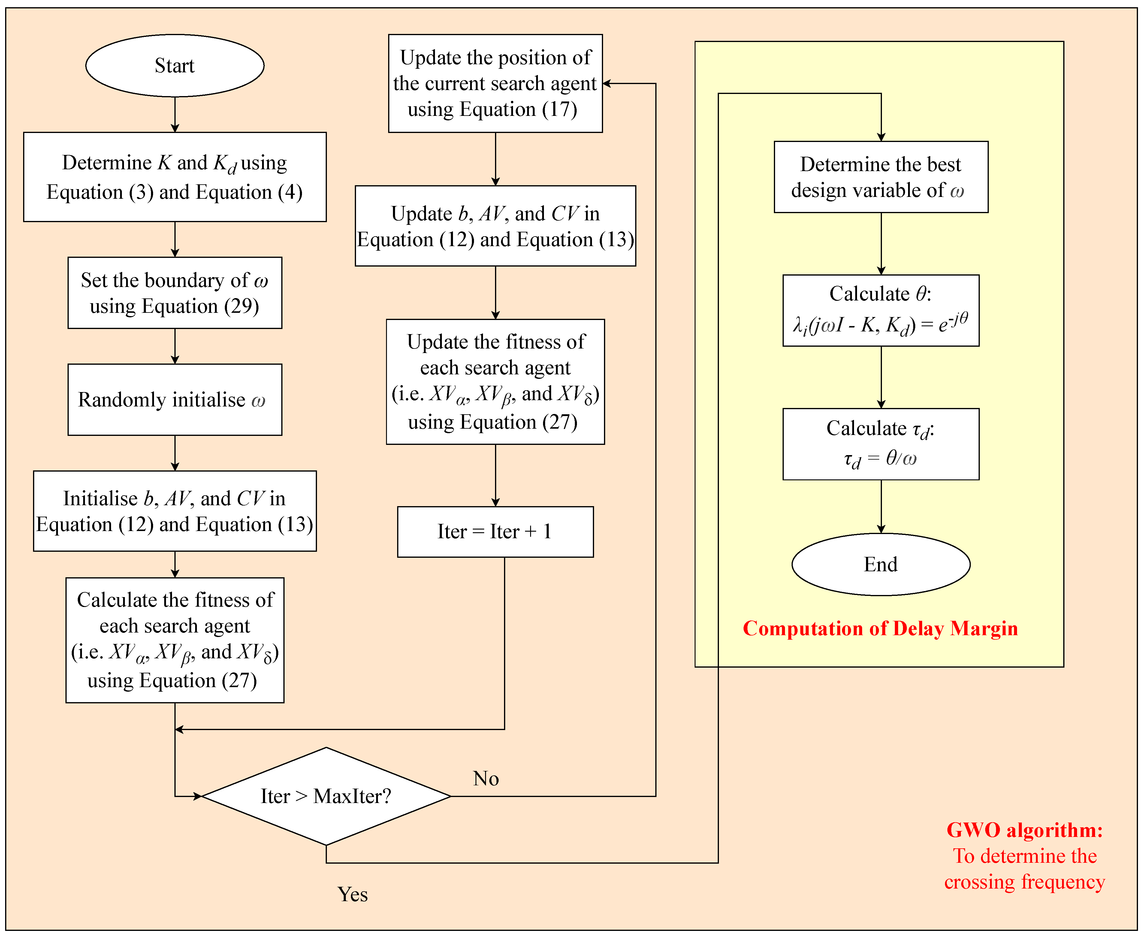
4. Delay Margin Computation Based on Grey Wolf Optimisation
- K is stable;
- K + is stable, and;
- > 1, > 0.
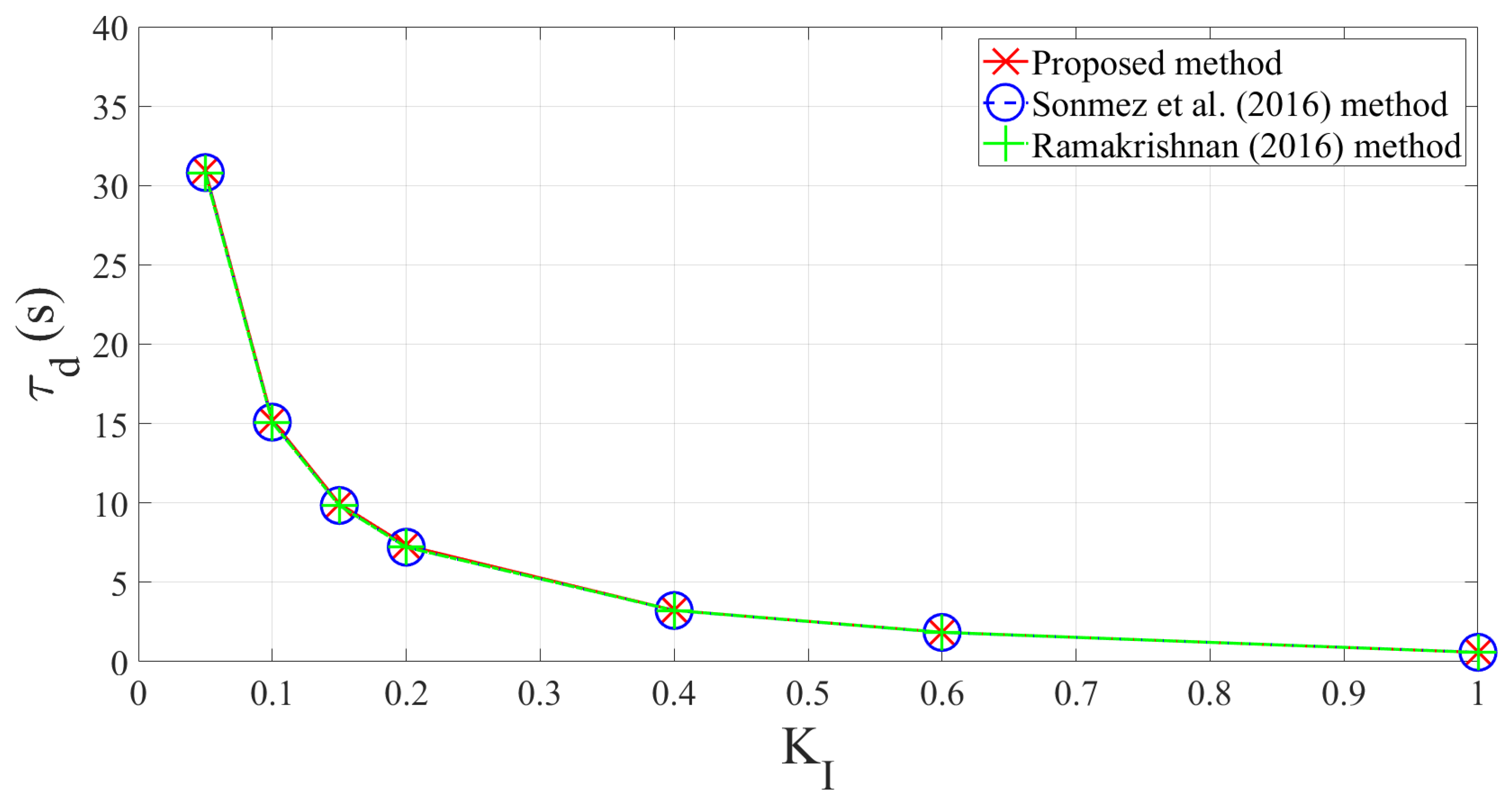
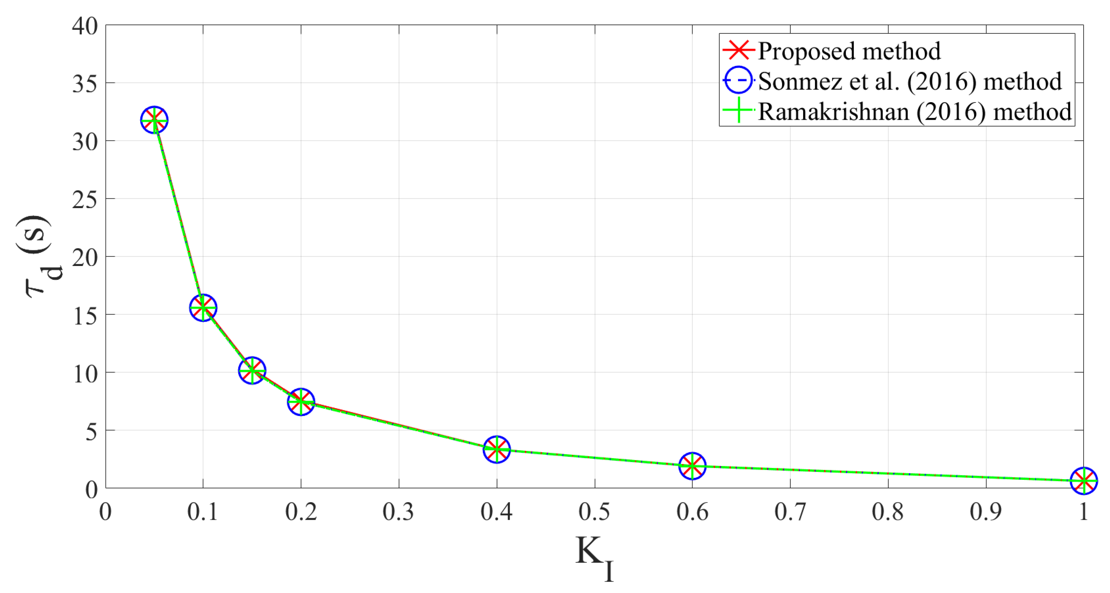
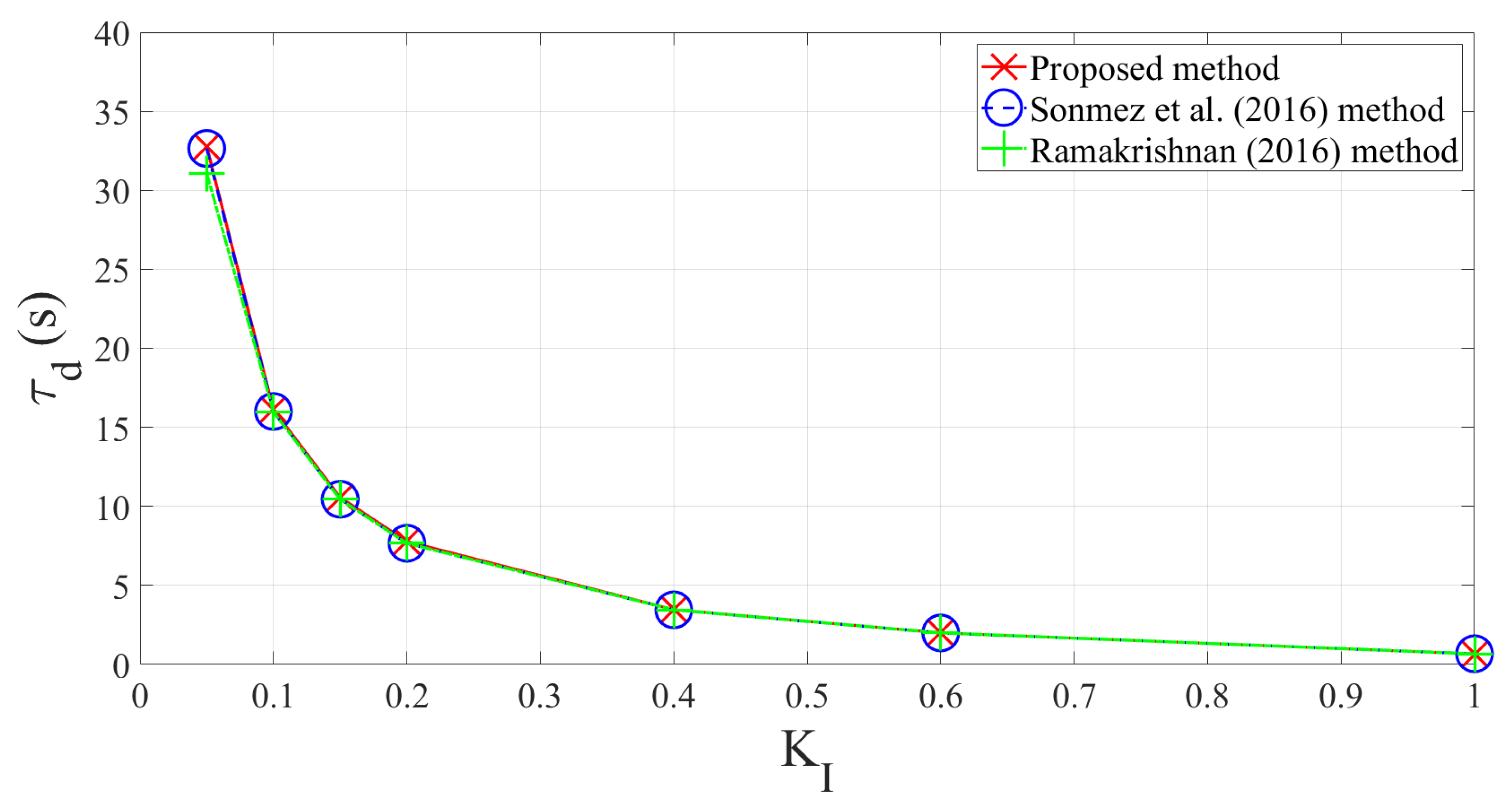
5. Case Study: Two-Area LFC System
6. Conclusions
Author Contributions
Funding
Data Availability Statement
Conflicts of Interest
References
- Saadat, H. Power System Analysis; McGraw-Hill Companies: New York, NY, USA, 1999. [Google Scholar]
- Xu, X.; Tomsovic, K. Application of Linear Matrix Inequalities for Load Frequency Control with Communication Delays. IEEE Trans. Power Syst. 2004, 19, 1508–1515. [Google Scholar]
- Mak, K.H.; Holland, B.L. Migrating electrical power network SCADA systems to TCP/IP and Ethernet networking. Power Eng. J. 2002, 16, 305–311. [Google Scholar]
- Gu, K.; Niculescu, S.I. Survey on Recent Results in the Stability and Control of Time-Delay Systems. J. Dyn. Sys. Meas. Control. 2003, 125, 158–165. [Google Scholar] [CrossRef]
- Yan, S.; Gu, Z.; Park, J.H.; Xie, X.; Dou, C. Probability-density-dependent load frequency control of power systems with random delays and cyber-attacks via Circuital implementation. IEEE Trans. Smart Grid 2022, 13, 4837–4847. [Google Scholar] [CrossRef]
- Yang, F.; He, J.; Pan, Q. Further Improvement on Delay-Dependent Load Frequency Control of Power Systems via Truncated B-L Inequality. IEEE Trans. Power Syst. 2018, 33, 5062–5071. [Google Scholar] [CrossRef]
- Çelik, V.; Özdemir, M.T.; Lee, K.Y. Effects of Fractional-Order Pi Controller on Delay Margin in Single-Area Delayed Load Frequency Control Systems. J. Mod. Power Syst. Clean Energy 2018, 7, 380–389. [Google Scholar] [CrossRef]
- Shen, L.; Xiao, H. Delay-Dependent Robust Stability Analysis of Power Systems with PID Controller. Chin. J. Electr. Eng. 2019, 5, 79–86. [Google Scholar] [CrossRef]
- Jin, L.; Zhang, C.-K.; He, Y.; Jiang, L.; Wu, M. Delay-Dependent Stability Analysis of Multi-Area Load Frequency Control with Enhanced Accuracy and Computation Efficiency. IEEE Trans. Power Syst. 2019, 34, 3687–3696. [Google Scholar] [CrossRef]
- Shen, C.; Li, Y.; Zhu, X.; Duan, W. Improved Stability Criteria for Linear Systems with Two Additive Time-Varying Delays via a Novel Lyapunov Functional. J. Comput. Appl. Math. 2020, 363, 312–324. [Google Scholar] [CrossRef]
- Chen, W.; Gao, F.; Liu, G. New Results on Delay-Dependent Stability for Nonlinear Systems with Two Additive Time-Varying Delays. Eur. J. Control. 2021, 58, 123–130. [Google Scholar] [CrossRef]
- Arunagirinathan, S.; Muthukumar, P. New Asymptotic Stability Criteria for Time-Delayed Dynamical Systems with Applications in Control Models. Results Control. Optim. 2021, 3, 100014. [Google Scholar] [CrossRef]
- Feng, W.; Xie, Y.; Luo, F.; Zhang, X.; Duan, W. Enhanced Stability Criteria of Network-Based Load Frequency Control of Power Systems with Time-Varying Delays. Energies 2021, 14, 5820. [Google Scholar] [CrossRef]
- Liu, X.; Shi, K.; Tang, L.; Tang, Y. Further Improvement on Stability Results for Delayed Load Frequency Control System via Novel Lkfs and Proportional-Integral Control Strategy. Discret. Dyn. Nat. Soc. 2022, 2022, 4798415. [Google Scholar] [CrossRef]
- Li, Y.; Qiu, T.; Yang, Y. Delay-Dependent Stability Criteria for Linear Systems with Two Additive Time-Varying Delays. Int. J. Control. Autom. Syst. 2022, 20, 392–402. [Google Scholar] [CrossRef]
- Khalil, A.; Swee Peng, A. A New Method for Computing the Delay Margin for the Stability of Load Frequency Control Systems. Energies 2018, 11, 3460. [Google Scholar] [CrossRef]
- Khalil, A.; Laila, D.S. An Accurate Method for Computing the Delay Margin in Load Frequency Control System with Gain and Phase Margins. Energies 2022, 15, 3434. [Google Scholar] [CrossRef]
- Sonmez, S.; Ayasun, S.; Nwankpa, C.O. An Exact Method for Computing Delay Margin for Stability of Load Frequency Control Systems with Constant Communication Delays. IEEE Trans. Power Syst. 2016, 31, 370–377. [Google Scholar] [CrossRef]
- Thangaiah, J.M.; Parthasarathy, R. Delay-Dependent Stability Analysis of Power System Considering Communication Delays. Int. Trans. Electr. Energy Syst. 2016, 27, e2260. [Google Scholar] [CrossRef]
- Ibrahim, M.H.; Ang, S.P.; Dani, M.N.; Rahman, M.I.; Petra, R.; Sulthan, S.M. Optimizing Step-Size of Perturb & Observe and Incremental Conductance MPPT Techniques Using PSO for Grid-Tied PV System. IEEE Access 2023, 11, 13079–13090. [Google Scholar] [CrossRef]
- Shehata, A.A.; Tolba, M.A.; El-Rifaie, A.M.; Korovkin, N.V. Power System Operation Enhancement using a new hybrid methodology for optimal allocation of FACTS devices. Energy Rep. 2022, 8, 217–238. [Google Scholar] [CrossRef]
- Sheikhzadeh-Baboli, P.; Assili, M. A hybrid adaptive algorithm for power system frequency restoration based on proposed emergency demand side management. IETE J. Res. 2021, 1–13. [Google Scholar] [CrossRef]
- Nadimi-Shahraki, M.H.; Taghian, S.; Mirjalili, S.; Abualigah, L.; Abd Elaziz, M.; Oliva, D. EWOA-OPF: Effective Whale Optimization Algorithm to Solve Optimal Power Flow Problem. Electronics 2021, 10, 2975. [Google Scholar] [CrossRef]
- Nadimi-Shahraki, M.H.; Taghian, S.; Mirjalili, S.; Faris, H. MTDE: An effective multi-trial vector based differential evolution algorithm and its applications for engineering design problems. Appl. Soft Comput. 2020, 97, 106761. [Google Scholar] [CrossRef]
- Nadimi-Shahraki, M.H.; Taghian, S.; Mirjalili, S. An improved grey wolf optimizer for solving engineering problems. Expert Syst. Appl. 2021, 166, 113917. [Google Scholar] [CrossRef]
- Nadimi-Shahraki, M.H.; Moeini, E.; Taghian, S.; Mirjalili, S. DMFO-CD: A Discrete Moth-Flame Optimization Algorithm for Community Detection. Algorithms 2021, 14, 314. [Google Scholar] [CrossRef]
- Nadimi-Shahraki, M.H.; Taghian, S.; Mirjalili, S.; Ewees, A.A.; Abualigah, L.; Abd Elaziz, M. MTV-MFO: Multi-Trial Vector-Based Moth-Flame Optimization Algorithm. Symmetry 2021, 13, 2388. [Google Scholar] [CrossRef]
- Ramakrishnan, K. Delay-dependent stability criterion for delayed load frequency control systems. In Proceedings of the IEEE Annual India Conference (INDICON), Bangalore, India, 16–18 December 2016; pp. 1–6. [Google Scholar]
- Jiang, L.; Yao, W.; Wu, Q.H.; Wen, J.Y.; Cheng, S.J. Delay-Dependent Stability for Load Frequency Control with Constant and Time-Varying Delays. IEEE Trans. Power Syst. 2012, 27, 932–941. [Google Scholar] [CrossRef]
- Manikandan, S.; Kokil, P. Delay-Dependent Stability Analysis of Network-Based Load Frequency Control of One and Two Area Power System with Time-Varying Delays. Fluct. Noise Lett. 2019, 18, 1950007. [Google Scholar] [CrossRef]
- Naduvathuparambil, B.; Valenti, M.C.; Feliachi, A. Communication delays in wide area measurement systems. In Proceedings of the Thirty-Fourth Southeastern Symposium on System Theory, Huntsville, Alabama, 18–19 March 2002; pp. 118–122. [Google Scholar]
- Mirjalili, S.; Mirjalili, S.M.; Lewis, A. Grey Wolf Optimizer. Adv. Eng. Softw. 2014, 69, 46–61. [Google Scholar] [CrossRef]
- Ibrahim, M.H.; Ang, S.P.; Hamid, Z.; Mohammed, S.S.; Law, K.H. A Comparative Hybrid Optimisation Analysis of Load Frequency Control in a Single Area Power System Using Metaheuristic Algorithms and LQR. In Proceedings of the 2022 International Conference on Green Energy, Computing, and Sustainable Technology (GECOST 2022), Miri, Sarawak, Malaysia, 26–28 October 2022; pp. 227–232. [Google Scholar]
- Gu, K.; Kharitonov, V.L.; Chen, J. Stability of Time-Delay Systems; Springer: Berlin/Heidelberg, Germany, 2003. [Google Scholar]
- Chen, J. On Computing the Maximal Delay Intervals for Stability of Linear Delay Systems. IEEE Trans. Autom. Control 1995, 40, 1087–1093. [Google Scholar] [CrossRef]
- Chen, J.; Latchman, H.A. Frequency Sweeping Tests for Stability Independent of Delay. IEEE Trans. Autom. Control 1995, 40, 1640–1645. [Google Scholar] [CrossRef]
- Chen, J.; Gu, G.; Nett, C.N. A New Method for Computing Delay Margins for Stability of Linear Delay Systems. In Proceedings of the IEEE 33rd Conference on Decision and Control, Lake Buena Vista, FL, USA, 14–16 December 1994; pp. 433–437. [Google Scholar]


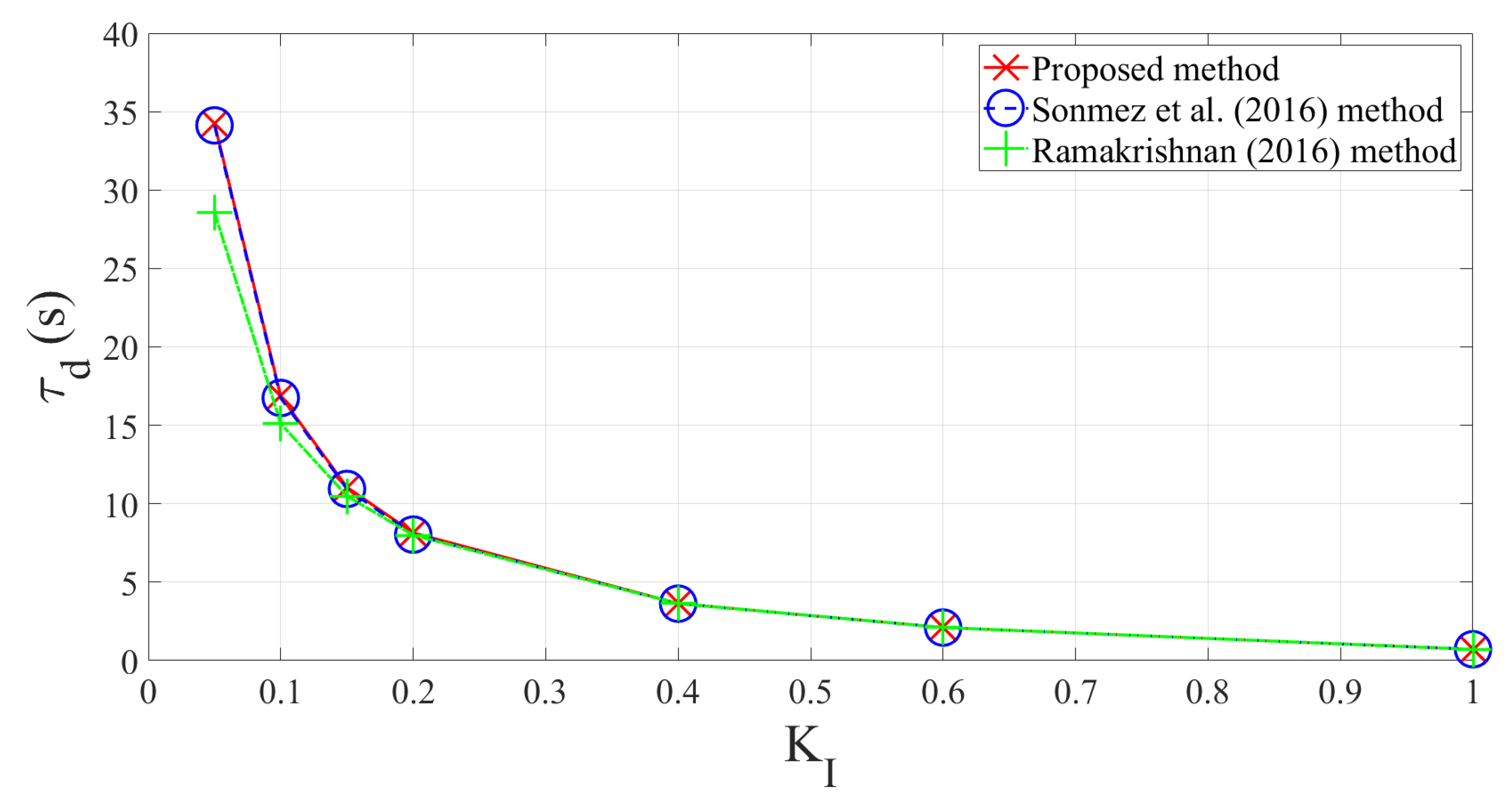
| Method | 0.05 | 0.10 | 0.15 | 0.20 | 0.40 | 0.60 | 1.0 | |
|---|---|---|---|---|---|---|---|---|
| Proposed method | 30.935 | 15.200 | 9.949 | 7.322 | 3.235 | 1.851 | 0.586 | |
| [18] | 30.812 | 15.090 | 9.842 | 7.211 | 3.225 | 1.843 | 0.591 | |
| 0.0 | [19] | 30.827 | 15.178 | - | 7.225 | 3.275 | 1.930 | - |
| [28] | 30.756 | 15.072 | 9.835 | 7.210 | 3.231 | 1.849 | 0.586 | |
| [29] | 27.848 | 13.699 | 8.974 | 6.603 | 3.002 | 1.745 | 0.573 | |
| Proposed method | 31.895 | 15.680 | 10.269 | 7.561 | 3.354 | 1.930 | 0.631 | |
| [18] | 31.772 | 15.570 | 10.162 | 7.450 | 3.345 | 1.922 | 0.638 | |
| 0.05 | [19] | 31.763 | 15.587 | - | 7.509 | 3.399 | 2.008 | - |
| [28] | 31.704 | 15.547 | 10.152 | 7.448 | 3.350 | 1.928 | 0.631 | |
| [29] | 27.830 | 14.020 | 9.205 | 6.777 | 3.095 | 1.810 | 0.616 | |
| Proposed method | 32.772 | 16.117 | 10.560 | 7.780 | 3.462 | 2.000 | 0.669 | |
| [18] | 32.647 | 16.008 | 10.453 | 7.669 | 3.453 | 1.993 | 0.676 | |
| 0.10 | [19] | 32.632 | 16.021 | - | 7.700 | 3.507 | 2.079 | - |
| [28] | 31.083 | 15.968 | 10.440 | 7.664 | 3.457 | 1.998 | 0.669 | |
| [29] | 27.001 | 13.650 | 9.166 | 6.881 | 3.174 | 1.863 | 0.649 | |
| Proposed method | 34.248 | 16.852 | 11.050 | 8.146 | 3.641 | 2.113 | 0.716 | |
| [18] | 34.122 | 16.744 | 10.943 | 8.035 | 3.631 | 2.106 | 0.725 | |
| 0.20 | [19] | 34.1563 | 16.768 | - | 8.058 | 3.694 | 2.1975 | - |
| [28] | 28.579 | 15.102 | 10.495 | 7.998 | 3.634 | 2.110 | 0.716 | |
| [29] | 25.090 | 12.702 | 8.572 | 6.497 | 3.209 | 1.931 | 0.692 | |
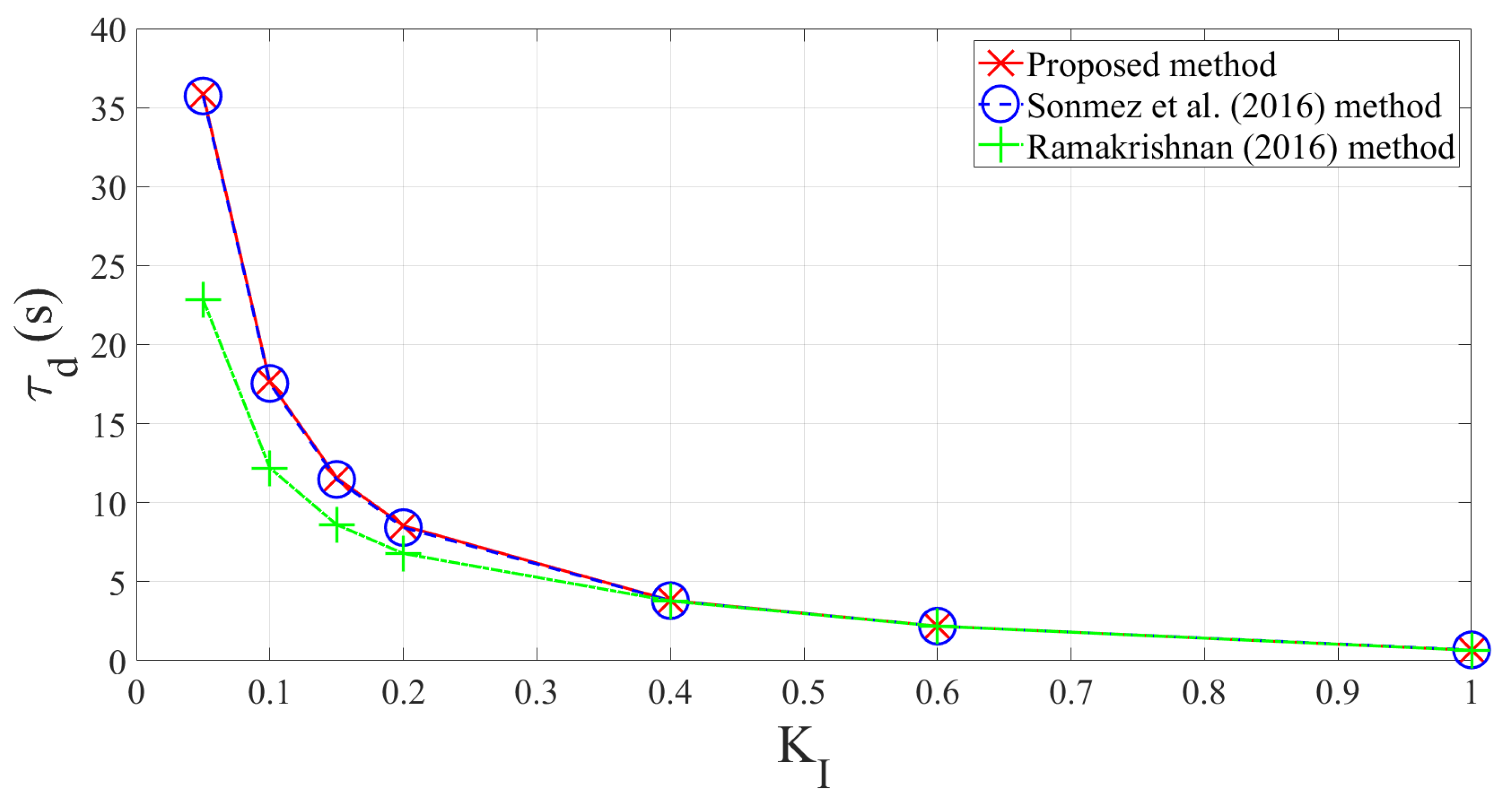
| Proposed method | 35.845 | 17.647 | 11.574 | 8.536 | 3.812 | 2.189 | 0.662 | |
| [18] | 35.728 | 17.542 | 11.469 | 8.424 | 3.802 | 2.184 | 0.684 | |
| 0.40 | [19] | 35.7223 | 17.566 | - | 8.4673 | 3.876 | 2.2997 | - |
| [28] | 22.841 | 12.196 | 8.609 | 6.781 | 3.778 | 2.184 | 0.662 | |
| [29] | 20.278 | 10.364 | 7.014 | 5.338 | 2.735 | 1.731 | 0.637 | |
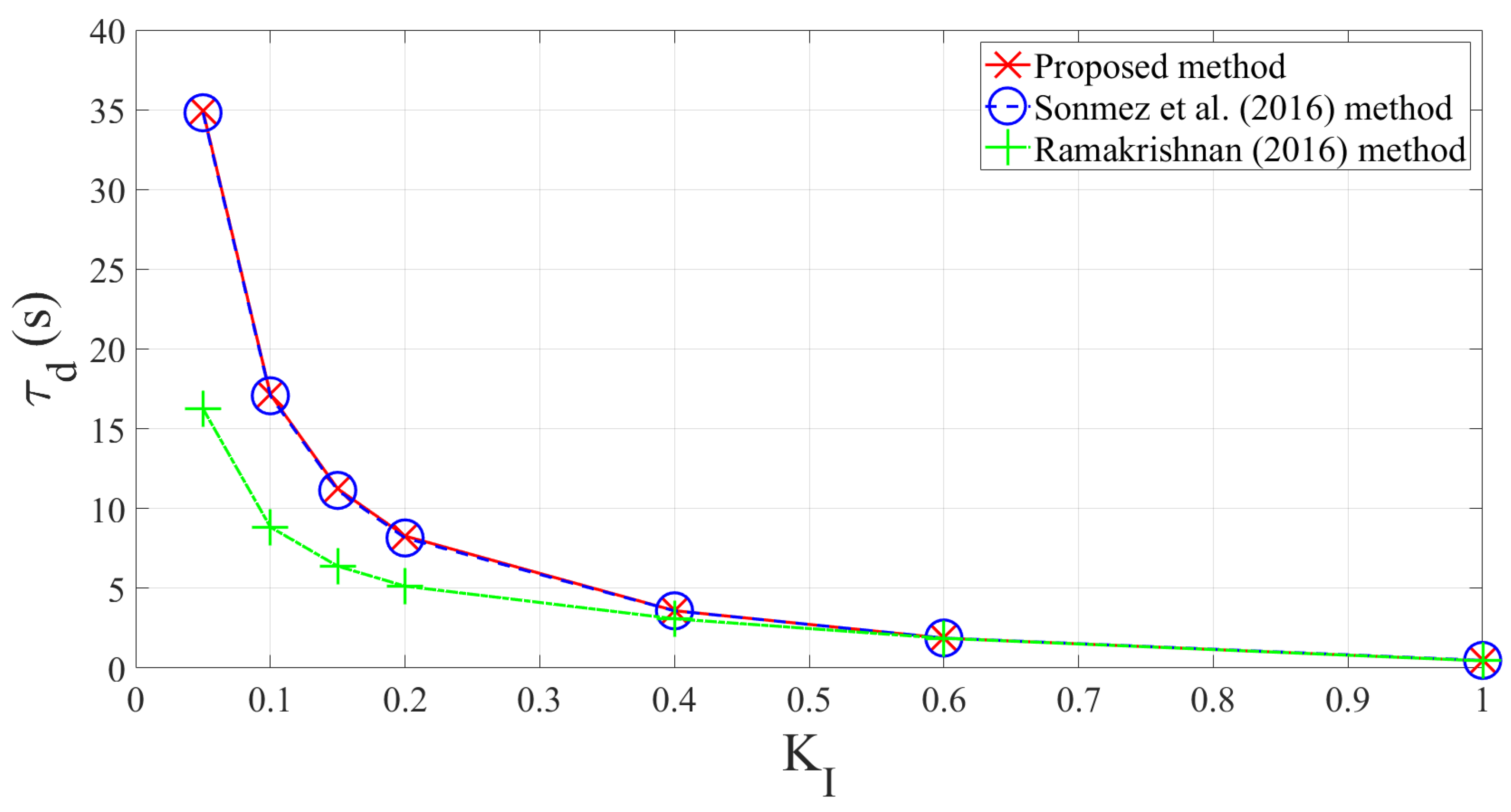
| Proposed method | 34.914 | 17.162 | 11.239 | 8.275 | 3.597 | 1.874 | 0.454 | |
| [18] | 34.809 | 17.068 | 11.136 | 8.155 | 3.588 | 1.881 | 0.480 | |
| 0.60 | [19] | 34.8393 | 17.103 | - | 8.2113 | 3.710 | 2.1141 | - |
| [28] | 16.254 | 8.839 | 6.387 | 5.134 | 3.089 | 1.864 | 0.454 | |
| [29] | 14.228 | 7.332 | 4.944 | 3.768 | 1.920 | 1.198 | 0.443 | |
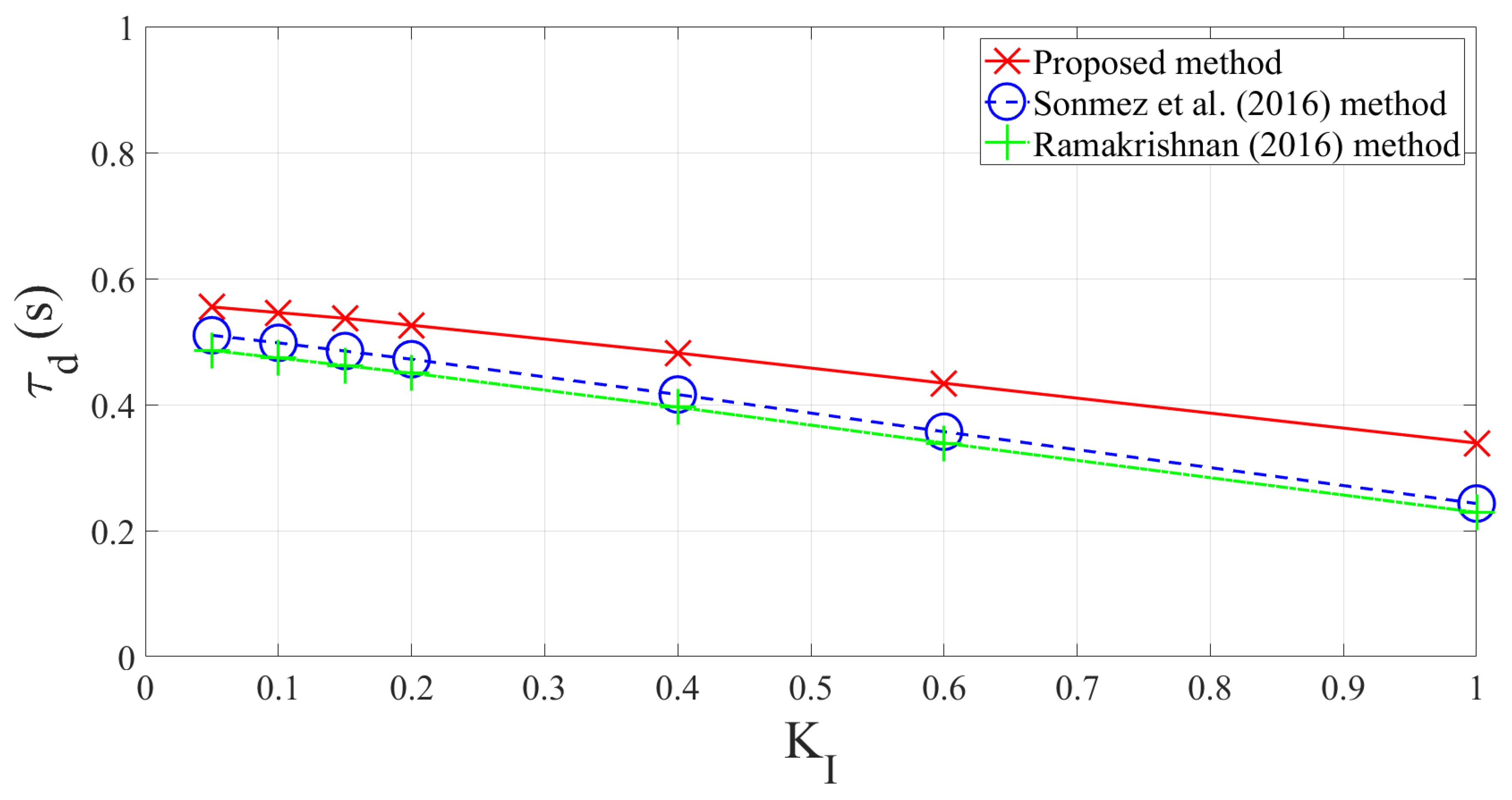
| Proposed method | 0.555 | 0.546 | 0.537 | 0.526 | 0.482 | 0.434 | 0.339 | |
| [18] | 0.510 | 0.498 | 0.485 | 0.472 | 0.416 | 0.357 | 0.243 | |
| 1.0 | [19] | - | - | - | - | - | - | - |
| [28] | 0.486 | 0.474 | 0.462 | 0.450 | 0.396 | 0.339 | 0.229 | |
| [29] | 0.465 | 0.455 | 0.444 | 0.433 | 0.384 | 0.332 | 0.227 | |
Disclaimer/Publisher’s Note: The statements, opinions and data contained in all publications are solely those of the individual author(s) and contributor(s) and not of MDPI and/or the editor(s). MDPI and/or the editor(s) disclaim responsibility for any injury to people or property resulting from any ideas, methods, instructions or products referred to in the content. |
© 2023 by the authors. Licensee MDPI, Basel, Switzerland. This article is an open access article distributed under the terms and conditions of the Creative Commons Attribution (CC BY) license (https://creativecommons.org/licenses/by/4.0/).
Share and Cite
Ibrahim, M.H.; Peng, A.S.; Dani, M.N.; Khalil, A.; Law, K.H.; Yunus, S.; Rahman, M.I.; Au, T.W. A Novel Computation of Delay Margin Based on Grey Wolf Optimisation for a Load Frequency Control of Two-Area-Network Power Systems. Energies 2023, 16, 2860. https://doi.org/10.3390/en16062860
Ibrahim MH, Peng AS, Dani MN, Khalil A, Law KH, Yunus S, Rahman MI, Au TW. A Novel Computation of Delay Margin Based on Grey Wolf Optimisation for a Load Frequency Control of Two-Area-Network Power Systems. Energies. 2023; 16(6):2860. https://doi.org/10.3390/en16062860
Chicago/Turabian StyleIbrahim, Mohammad Haziq, Ang Swee Peng, Muhammad Norfauzi Dani, Ashraf Khalil, Kah Haw Law, Sharina Yunus, Mohammad Ishlah Rahman, and Thien Wan Au. 2023. "A Novel Computation of Delay Margin Based on Grey Wolf Optimisation for a Load Frequency Control of Two-Area-Network Power Systems" Energies 16, no. 6: 2860. https://doi.org/10.3390/en16062860
APA StyleIbrahim, M. H., Peng, A. S., Dani, M. N., Khalil, A., Law, K. H., Yunus, S., Rahman, M. I., & Au, T. W. (2023). A Novel Computation of Delay Margin Based on Grey Wolf Optimisation for a Load Frequency Control of Two-Area-Network Power Systems. Energies, 16(6), 2860. https://doi.org/10.3390/en16062860