To Charge or to Sell? EV Pack Useful Life Estimation via LSTMs, CNNs, and Autoencoders

Abstract

Electric vehicles (EVs) are spreading fast as they promise to provide better performance and comfort, but above all, to help face climate change. Despite their success, their cost is still a challenge. Lithium-ion batteries are one of the most expensive EV components, and have become the standard for energy storage in various applications. Precisely estimating the remaining useful life (RUL) of battery packs can encourage their reuse and thus help to reduce the cost of EVs and improve sustainability. A correct RUL estimation can be used to quantify the residual market value of the battery pack. The customer can then decide to sell the battery when it still has a value, i.e., before it exceeds the end of life of the target application, so it can still be reused in a second domain without compromising safety and reliability. This paper proposes and compares two deep learning approaches to estimate the RUL of Li-ion batteries: LSTM and autoencoders vs. CNN and autoencoders. The autoencoders are used to extract useful features, while the subsequent network is then used to estimate the RUL. Compared to what has been proposed so far in the literature, we employ measures to ensure the method’s applicability in the actual deployed application. Such measures include (1) avoiding using non-measurable variables as input, (2) employing appropriate datasets with wide variability and different conditions, and (3) predicting the remaining ampere-hours instead of the number of cycles. The results show that the proposed methods can generalize on datasets consisting of numerous batteries with high variance.

1. Introduction and Background

Electric vehicles (EVs) are becoming central to the automotive industry as they can address current automotive limits. Their constant growth is due to their improved performance and efficiency, but especially for their suitability in addressing environmental challenges, i.e., urban pollution and global warming [1,2]. Internal-combustion-based vehicles contribute to global carbon emissions by 14% of the total [3]; thus, they are facing restrictions in leading markets that aim to reduce their environmental footprint [2,4]. Internal-combustion-based vehicles are also a prominent source of artificial fine particulate matter ($P{M}_{2.5}$) [5,6]. Air pollution is one of our greatest social issues since it has a severe impact on health and society [7], possibly causing different diseases and even premature death [8,9]. EVs are a milestone in addressing such challenges to humanity as they can potentially remove personal transportation from the environmental impact equation.

A core component of EVs is the battery. Lithium-ion (Li-ion) batteries have become the standard for energy storage in EVs [10,11]. They have several advantages compared to traditional batteries such as lead-acid or nickel-metal hydride: high energy and power density, low self-discharge, environmental adaptability, long lifetimes, and high reliability [12,13]. These advantages have led to the wide use of Li-ion batteries in EVs and in several safety-critical areas such as space applications [14], aircraft, and backup energy systems. The safety and reliability of Li-ion batteries are critical concerns for such applications [15]. Li-ion batteries are employed in safety-critical areas, so their defects can cause fatal system failures. For example, various Boeing 787 aircraft caught fire because of Li-ion battery malfunctions in 2013 [16], and NASA lost a spacecraft because of the lack of power supply due to a false battery over-charging indication in 2006 [17]. Such high-impact failures have also recently appeared in the EV domain, with well-known manufacturers recalling hundreds of thousands of EVs due to fire risk [18,19]. Another far more significant challenge for Li-ion batteries is their cost. While EVs are promising on various fronts, their cost is still a considerable drawback [20], and the battery is one of the most expensive components of EVs [21].

The design of an appropriate battery management system (BMS) is crucial to reducing costs and increasing vehicle efficiency and security [22,23]. One of the major tasks of the BMS is to evaluate the current health conditions of the battery as it degrades over time. This degradation is an irreversible process related to the repetitive charging and discharging operations and electrochemical reactions inside the battery [24]. Predominant indicators are battery capacity and internal resistance, which inform us about the battery residual energy and power capabilities, respectively [25], indicated by the state of health (SOH). The SOH and the remaining useful life (RUL) are the most crucial parameters of battery health that must be estimated by the BMS [12]. The SOH quantifies the deterioration level compared to a brand new battery. While it has not been formally defined by industry [26], it is typically expressed through a percentage of capacity loss or power loss (increase in battery resistance) [27,28]. We will consider the capacity loss (SOHc), which is defined by

$$SOH=\frac{C_t}{C_0}·100(\%)$$

(1)

where $C_t$ is the current capacity and $C_0$ is the nominal capacity. The International Electrotechnical Commission (IEC) [29], International Organization for Standardization (ISO) [30], and Institute of Electrical and Electronics Engineers Standards Association (IEEE-SA) [31] have proposed standards to measure the battery capacity in a standard condition using direct methods that are taken as a reference to compute $C_t$ and $C_0$. The BMS adjusts its functioning according to the estimated SOH to ensure vehicle performance and safety until the health indicators reach the target limits, after which the battery should be replaced. Battery manufacturers usually set the capacity threshold under which the battery is no longer suitable for EV applications to 80% of the nominal capacity [32], measured under a standardized test. Such threshold is called the end-of-life (EOL). Despite this, the battery might be replaced before the threshold if the internal resistance rises above a normal level [25]. The threshold is also recommended to be 80% by the Center for Advanced Life Cycle Engineering (CALCE) at the University of Maryland [33] and 70% by NASA’s Prognostics Center of Excellence (PCoE) [34]. In the context of replacement and secondary use planning, it is helpful to predict how the SOH will evolve through time and when the battery will reach its EOL. This is defined by the RUL, which is typically described as the number of cycles remaining until EOL [35,36,37].

A robust SOH estimation by the BMS is fundamental to ensure battery reliability as well as prevent failures and hazards [22,38], but also to determine the acceleration performance and the driving range of the EV [39,40], necessary for a pleasant driving experience, and finally to quantify the residual market value of the batteries [41]. However, the correct estimation of the RUL encourages the reuse of batteries, as removing the battery before it exceeds the end of life of the target application allows reuse in a second domain without compromising safety and reliability [42]. Batteries can therefore be employed in secondary applications with lower power requirements. This can have a significant impact in terms of both sustainability and market value [43]. With the growing number of new EVs, the waste produced by the spent battery packages is also increasing. Their recycling processes can have a considerable economic and environmental impact. The interested reader is referred to [44] for lithium-ion battery recycling in the EV context. To summarize, improving the estimation of SOH and RUL contributes to the spreading of EVs in two ways: (1) by ensuring security and reliability, (2) by reducing costs and waste through battery reuse.

The estimation of the SOH and its prediction (the RUL) is a challenging task. The capacity of a cell cannot be directly measured, so indirect measurements are used instead by using related variables. The SOH can be precisely computed in laboratory conditions, but it significantly differs from the working conditions of real applications [25]. This, unfortunately, does not apply to the real-world EVs that have to employ online estimation algorithms [22]. Battery aging involves many variables, such as charge/discharge current, voltage, and operating temperature. EV batteries’ working conditions are also highly dynamic as they change with the environment and the user’s driving style [39]. As a result, it is challenging to design accurate physical models due to complex degradation mechanisms and operations. Furthermore, it requires much knowledge about the phenomena involved and experimental data acquired in controlled situations, which could be unavailable or quite expensive to collect [42]. SOH estimation techniques can be classified into two macro-categories: experimental and model-based estimation methods [22,25]. Experimental methods analyze aging behavior through numerous laboratory tests. As mentioned above, this is typically not achievable on board due to the required equipment and the dynamic driving context. Model-based methods can be further divided into adaptive algorithms and data-driven approaches, and the latter also includes RUL prediction. Adaptive algorithms use mathematical models and numerical filters (e.g., equivalent circuit model and Kalman filters). In contrast, data-driven methods use black box models, which find the mapping between the input and the target. Figure 1 summarizes the main categories of SOH estimation methods. The following section will focus on machine-learning-based SOH estimation and RUL prediction techniques and their advantages. For a detailed review of the other methods for SOH estimation, please refer to [25], and for RUL prediction, please refer to [45].

This paper contributes in several directions to the applicability of deep-learning-based RUL estimation in practical applications.

• We propose a novel RUL definition in the machine learning context, based on ampere-hours, to push forward the applicability to real cases. The first application of deep learning techniques on an RUL that is not based on the simplified concept of cycles is also provided.
• Two models for RUL estimation are presented and compared on the NASA Randomized dataset: autoencoder plus CNN and autoencoder plus LSTM. In addition, an LSTM is proposed to predict the RUL in the UNIBO Powertools dataset. The results show that the particular autoencoder can effectively extract the relevant features of the cycle curves, while the CNNs and the LSTMs can be used to estimate the RUL.
• Two vast datasets containing batteries cycled with an extensive set of different conditions and variables are used in the experiments to ensure generalization. Compared to the data used in the literature so far (with a limited amount of batteries typically discharged under constant current), the examples used in this paper present many more batteries and conditions that are more challenging to predict. All the relevant details about the data selection and splitting are detailed, ensuring transparency in the results.

The paper is structured as follows. The next section provides an overview of the deep-learning-based techniques used for RUL estimation and the problems that affect their deployment. The relevant works are also summarized. In Section 3, the datasets and the models used are described. Section 4 shows and compares the results obtained using the models. Finally, Section 5 concludes the paper with a summary of the results and future research directions.

2. Related Works

The recent success of machine learning in several domains and the availability of data and computing power have motivated the development of novel methods for battery state estimation. Data-driven battery state estimation methods are becoming increasingly popular [28]. In particular, the attention to using deep learning (DL) for battery status estimation has increased over time. Data-driven methods provide several advantages [22]. They allow us to obtain better results in real complex applications, as complete knowledge about degradation mechanisms is still lacking. They do not require expert knowledge about the degradation phenomena as they only rely on enough operational data from which key features are extracted. They are also suitable for execution on hardware with limited capabilities compared to adaptive algorithms that are more computationally demanding [40,46]. While the training phase is demanding as well, the execution is efficient and can run on BMS hardware, with inference models in the order of a few hundred megabytes [47]. Last but not least, data-driven methods enable the prediction of the SOH (i.e., the RUL), while other techniques are typically limited to estimating the current SOH.

Drawbacks are present, but the benefits compensate for them. The main drawbacks are limited interpretability and inaccessibility to physical parameters (e.g., internal resistance) [48]. Before proceeding, it is worth noting that we may have a conflict of terms. While, in the context of deep learning, “prediction” typically indicates the result of a neural network, in the context of signal processing, it means predicting the future value of a time series. In this paper, we will use the term estimation to indicate the estimation of the current SOH. In contrast, we will use the word prediction to indicate the expected RUL, as it can be conceived as the prediction of the future SOH.

In the last two years, numerous works using DL for SOH and RUL estimation have been proposed in the literature. In the following, the common approaches (and issues) in the various papers are first presented to avoid repetition, and then the single articles are analyzed.

The variables measured by the BMS are usually voltage (V), current (I), and temperature (T). Such variables are sampled at high rates during subsequent charge and discharge cycles, resulting in very long time series. The variables most used as input are voltage, current, and temperature, as they can capture the battery aging factors [40], but sometimes the sampling time and the state of charge (SOC; i.e., the charge level) are also used. In the case of the RUL, the SOH itself has also been used as input. It is recalled, however, that care must be taken when non-measured variables (i.e., SOC, SOH) are employed, as errors could accumulate and robust estimation of the input variable might not always be available— this is the first issue affecting applicability. The variables can originate from the charging cycles, the discharging cycles, or both. The resulting time series are often presented to the network through a moving window, i.e., the NN makes the estimation based on the set of features at time t plus their last N values. A popular approach is to use a recurrent neural network (RNN)—in one of its various forms—to find the relation between the SOH or RUL and the time series. Long short-term memory (LSTM) [49] networks are particular RNNs that are able to handle long-term sequences and have become the baseline of recurrent networks. LSTMs and their variants are thus also widely used in the battery context. Some experiments try instead to use convolutional neural networks (CNNs) to process time series, or to use a simple feed-forward NN (FFNN) preceded by specific pre-processing. The literature offers several battery datasets to conduct such experiments. One of the most used datasets is the NASA “Battery Data Set” [34]. It was the first battery dataset that was publicly available, and thus it has had a significant impact in the field [50]. The dataset consists of 34 Li-ion 18,650 cells cycled at various ambient temperatures; however, it includes only constant current (CC)-cycled batteries. Even though the dataset contains 34 batteries, the most common approach is to use a specific subset of three or four batteries. In 2014, NASA released another dataset (“Randomized Battery Usage Data Set”) [51] also containing batteries cycled with a random current. A review of battery datasets is available in [50]. The second issue to be addressed to ensure the suitability of the SOH and RUL methods to real scenarios is the quality of the dataset used during testing. Most works use simplified databases with batteries cycled under CC discharge, a condition not applicable to EV operation. Another applicability obstacle in the case of RUL is in the definition of RUL itself. As already mentioned, RUL is defined as the remaining cycles before EOL. In the EV context, we have partial charge and discharge cycles (e.g., discharge to 40%, charge to 80%, discharge to 30%, and so on) as the vehicle can be recharged starting from different SOCs and can be unplugged before the full charge. An equivalent full cycle (0% to 100%) has little practical meaning, therefore the definition of RUL has to be rethought. A valid candidate to represent the RUL in the EV setting is the remaining ampere-hour (Ah) value that the battery can deliver before reaching EOL. The measures to prevent applicability pitfalls are then (1) avoiding using non-measurable variables as input, (2) employing appropriate datasets with wide variability and different conditions, and (3) not using cycles to define the RUL.

The estimation of the SOH has recently become quite robust as it has been applied to realistic datasets. SOH estimation is well established on simplified datasets [22,28,52]; here, we report the recent advances on complex datasets. In [27], a hybrid network comprising a gated recurrent unit (GRU; a well-known variation of LSTM) and a CNN is used for SOH estimation. The inputs are the raw V, I, and T data of the charging curve, converted to a fixed size history of 256. The input converges toward the two parallel streams (GRU and CNN) concatenated in the last layer. A maximum estimation error of 4.3% on the Randomized NASA dataset is reported. The authors of [40] proposed an SOH estimation method based on the Independently RNN (IndRNN) and tested it on the Randomized NASA dataset. Here, a discharge cycle is represented by 18 features, including average V, I, and T, as well as the capacity, the time elapsed, and the time periods of each current load. While it achieves superior results, whether it will work in real applications needs to be clarified as it also takes capacity as input. In the experiments, the capacity in input is calculated. In contrast, the proper way to conduct the investigation should have used the capacity estimated by the network itself in the previous time step. In [42], a CNN takes as input the V, I, and capacity of the charging cycle discretized in 25 segments. The output is the capacity computed on the corresponding discharge cycle. Both capacities are computed by coulomb counting. Applicability is at least doubtful in this case too. In [39], a private database of real-world data collected from 700 vehicles (full-electric or hybrid) is used to train an FFNN for SOH estimation. The parameters employed are the accumulated mileage of cars, the C-rate distribution, the SOC range (the SOC is divided into five ranges, and the SOC range indicates such range), and cell temperatures. The number of variables is reduced to a lower dimensionality using principal component analysis (PCA). The results are impressive, with a maximum error of 4.5% and RMSE of 1.1%, which become 2.2% and 0.45% if considering only fully electric vehicles.

Moving to RUL estimation, it has not yet reached the robustness and applicability of SOH estimation. The experiments described in the literature are limited to oversimplified datasets that present only CC-cycled batteries. While adequate performances are typically achieved, there are still some critical issues regarding data quality and applicability. In [53], a temporal convolutional network (TCN) produces RUL estimations. The input is the history of the SOH, processed through a moving window. Tests are performed on three CC batteries from the NASA dataset and two CC batteries from the CALCE dataset. As it uses the history of SOH, a robust SOH estimation is necessary to ensure its applicability. As the experiments rely on ground truth SOH, it needs to be clarified if the proposed method will have the same performance using estimated SOH levels that are thus affected by some error. In addition, a long warm-up is required, as the first output is produced after a minimum t of 30 cycles. Both [54] and [55] propose using an LSTM network that takes the SOH’s history as input. In the first case, the output is the RUL; in the second case, it is the k-step ahead SOH, which can be reduced to the RUL. The datasets used are one Panasonic CC battery and four CC batteries from the NASA set, respectively. Both works present the same issues as the TCN-based one (here, the warm-up is even longer). The most promising article is [56], which presents a variant of LSTM, namely AST-LSTM. Two AST-LSTMs are trained, one for estimating the SOH and one for the RUL. The input of the first model includes V, I, T, and the sampling time of the discharge cycles. The second model uses instead the history of SOH estimated from the previous one. As the SOH input is estimated, the RUL approach is also suitable for real scenarios. Experiments are conducted on 12 batteries from the NASA dataset. The approach still needs to be tested on better datasets, and the warm-up is too long. In [13], the IC discharge curve is computed from the V, I, and sampling time. The features extracted from the curve are inputted to a small NN that estimates the SOH and RUL. This method is, however, applicable only to CC discharging. In addition, it has a high computation complexity and low performance. In [57], an autoencoder is used to perform dimensionality reduction starting from the V, I, T, and sampling time of both charge and discharge cycles, plus the capacity estimated during discharge. In addition to the applicability doubts, the accuracy is so low that the approach is substantially inapplicable. Another autoencoder approach from the same main author was proposed in [58]. Here, the autoencoder is used instead to augment the data dimension, and then the result is processed by two branches: an LSTM and a CNN. The features extracted by them are concatenated and fed to the final NN that returns the RUL prediction. While the performance has improved, the dataset used is still insufficient, as only CC-discharged batteries are considered. The properties of the above-mentioned works are summarized in

Table 1. Summary of current DL-based RUL estimation approaches.

Method	Input	Output	Dataset	Performances	Issues
TCN [53]	History of SOH	RUL	NASA, 3 CC batteries (#5, #6, #18) CALCE, 2 CC batteries (#CS_34, #CS_35)	RMSE up to 0.048	It requires a robust SOH estimation It is not clear if it will work if SOH is affected by errors Insufficient dataset variability Long warm-up (minimum starting cycle for NASA is 30 and the starting cycle for CALCE is 360)
LSTM network [54]	History of SOH	RUL	Panasonic 18,650 (1 CC battery)	-	It requires a robust SOH estimation It is not clear if it will work if SOH is affected by errors Insufficient dataset variability Long warm-up (start after 50% of battery life)
LSTM network [55]	History of SOH	K-step ahead SOH	NASA, 4 CC batteries (#5, #6, #7, #18)	MAE 1.92 (on battery #5)	It requires a robust SOH estimation It is not clear if it will work if SOH is affected by errors Insufficient dataset variability Long warm-up (start at cycle 60)
Variant of LSTM. SOH is estimated and then used to predict RUL [56]	V, I, T, sampling time (discharge)	SOH+RUL	NASA (12 batteries)	SOH: RMSE up to 0.059 RUL: RMSE up to 0.026 (on battery #5)	Insufficient dataset variability Long warm-up (start at cycle 50)
Features are extracted from the IC discharge curve and given as input to two NNs [13]	V, I, sampling time (discharge)	SOH+RUL	NASA, 4 CC batteries (#5, #6, #7, #18)	SOH: MRER up to 1.25% RUL: RMSE up to 5.41	Applicable only to CC discharging Computational complexity Insufficient dataset variability Low performances
Feature extraction with autoencoder followed by a DNN [57]	V, I, T, sampling time (charge + discharge), capacity, i.e., SOH (discharge)	RUL	NASA, 3 CC batteries (#5, #6, #7)	RMSE up to 13.2% (on battery #7)	It requires a robust SOH estimation It is not clear if it will work if SOH is affected by errors Insufficient dataset variability Insufficient performances
Auto-CNN-LSTM: data augmentation with autoencoder followed by CNN+LSTM extractor [58]	V, I, T, sampling time (charge + discharge)	RUL	NASA, 6 CC batteries (#5, #6, #7 #25, #27, #28)	RMSE up to 5.03% (on battery #7 and #28)	Insufficient dataset variability

.

3. Experiments

In this work, we propose and compare three models to predict the remaining useful life of Li-ion batteries. The contributions and improvements focus on the model’s applicability to real-world scenarios and the transparency in defining batteries and methodologies used. Existing works have used limited datasets without specifying why only some batteries from the selected dataset have been used. They also conform to the definition of RUL based on cycles, which has little meaning in actual applications. Finally, most of them do not provide enough information about the data structure and how data are employed. To achieve the desired aims, three aspects have been covered: input definition, output (RUL) definition, and the use of datasets with wide variability.

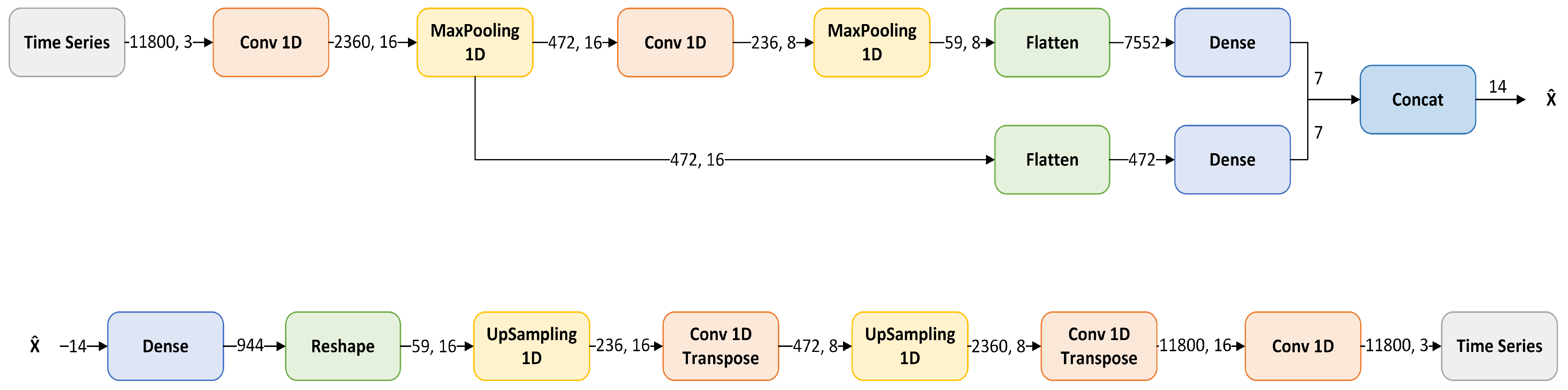
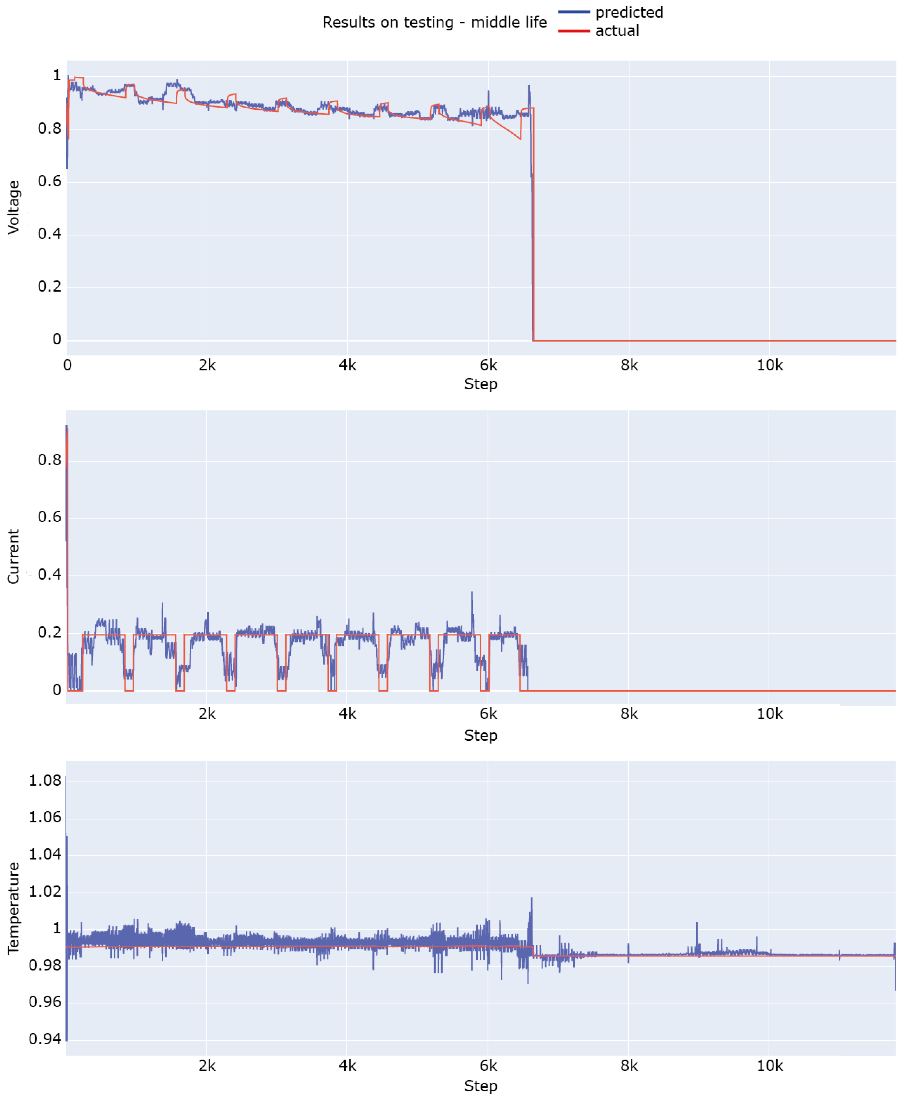
• Input: The only information used is voltage (V), current (I), and temperature (T), as using only measurable variables boosts applicability. The data are taken from the discharge cycles and are organized in time series, in the format $[cycle,timestep,variable]$. As explained in Section 3.2, at each cycle n, the input given to the network is based solely on the cycle n and the previous ones ($n-1,\dots ,n-N$; where N is the history length), i.e., no information from the future is used.
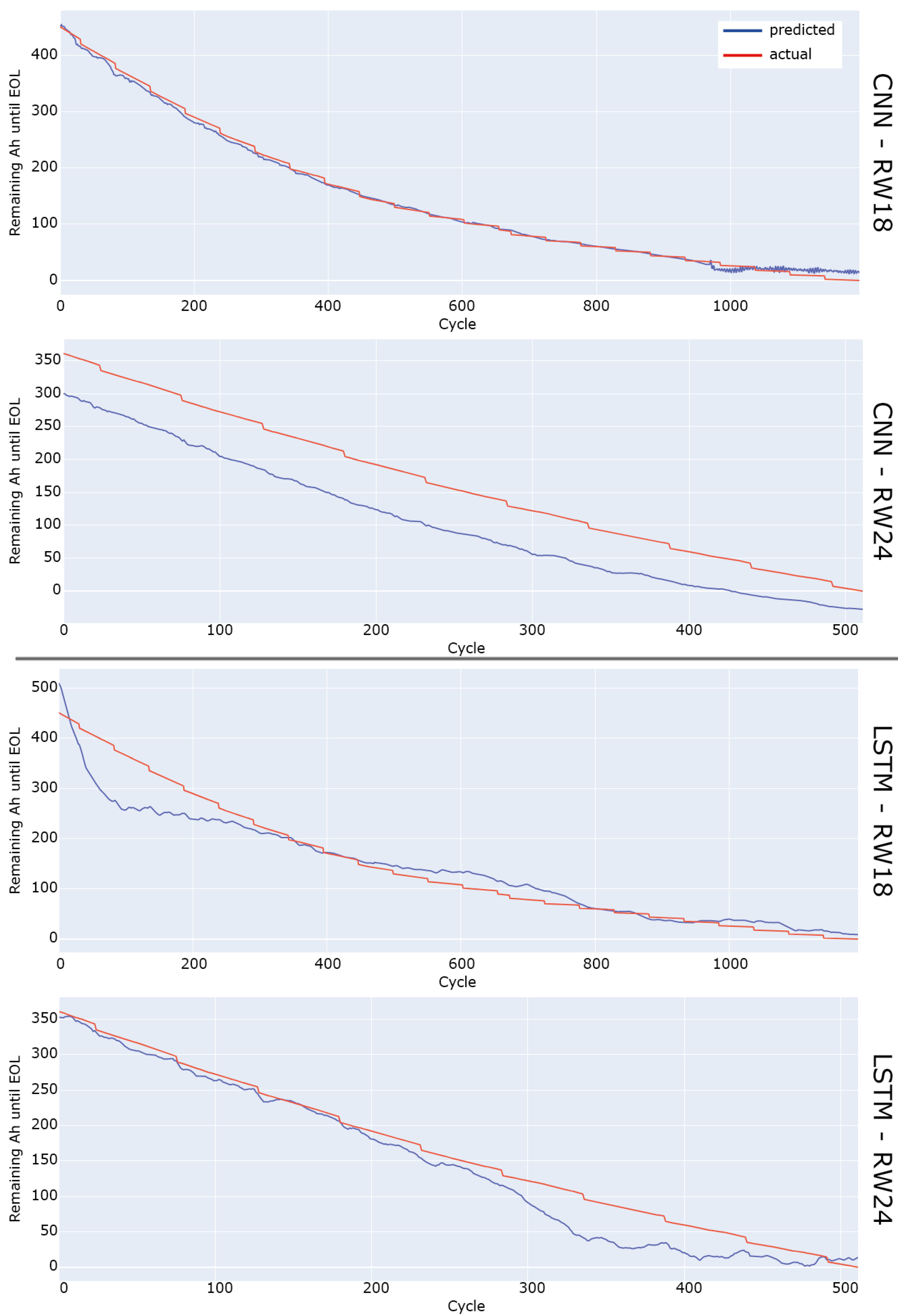
• Output—RUL definition: As detailed in Section 2, defining the RUL as the number of remaining cycles has no practical meaning. Here, instead, the RUL is defined as the normalized remaining ampere-hour (Ah) that the battery can deliver before reaching EOL.

This can be named ah-RUL and is computed as:

$$ahRUL\left(n\right)=[trapz(curren{t}_{[:,:]},tim{e}_{[:,:]})-trapz(curren{t}_{[n:EOL,:]},tim{e}_{[n:EOL,:]})]/nomcap$$

(2)

where n is the current cycle number, $trapz$ is the approximate integral via the trapezoidal method, $current$ is the matrix of currents where the x is the cycle and y is the timestep, $time$ is the matrix of the elapsed time corresponding to the current measurement, and $nomcap$ is the nominal capacity of the battery.

As the RUL is a slowly changing value, predicting at every cycle (rather than at each timestep) is more than sufficient. Thus, for each cycle n (and history N), the model predicts the ah-RUL at the current cycle.

The code for the pre-processing, as well as the networks, the trained models, the results, and the plots, are available in the repository of the project, which can be accessed at https://github.com/MichaelBosello/battery-rul-estimation (accessed on 15 March 2023).

3.1. Datasets

Two datasets have been used. The NASA Randomized Battery Usage dataset [51], which is used to investigate the performances of batteries cycled with a random current, and the UNIBO Powertools Dataset, which was released by our team in [59], and contains batteries with different specifications that were cycled under different conditions.

3.1.1. NASA Randomized Battery Usage Dataset

The NASA Randomized dataset consists of data from 28 batteries. The batteries are lithium cobalt oxide 18,650 cells with a nominal capacity of 2.2 Ah. The cells were continuously operated by repeatedly charging and discharging them according to the corresponding profile. At every 50 cycles, a series of reference charging and discharging cycles were performed to provide battery health status. The batteries are split into 7 groups containing 4 cells each according to the charge/discharge profile and temperature used. The randomized charge/discharge profiles can be as follows: random walk (RW), i.e., the selection of the current is random with a uniform distribution between the two current ranges; skewed RW, i.e., the current selection is random with a custom probability distribution skewed towards lower or higher currents.

• RW1, RW2, RW7, RW8 batteries are repeatedly charged for a random duration between 0.5 and 3 h, then discharged to 3.2 V using a randomized sequence of currents between 0.5 A and 4 A. The discharge random profile is the RW. The setpoint is loaded every 5 min. Operated at room temperature.
• RW3, RW4, RW5, RW6 batteries are repeatedly charged to 4.2 V and then discharged to 3.2 V using a randomized sequence of currents between 0.5 A and 4 A. The discharge random profile is the RW. The setpoint is loaded every 5 min. Operated at room temperature.
• RW9, RW10, RW11, RW12 batteries are repeatedly charged and then discharged using a randomized sequence of currents between −4.5 A and 4.5 A. The charge and discharge random profile is the RW. The setpoint is loaded every 5 min. Operated at room temperature.
• RW13, RW14, RW15, RW16 batteries are repeatedly charged to 4.2 V and then discharged to 3.2 V using a randomized sequence of currents between 0.5 A and 5 A. The random profile is the skewed high RW. The setpoint is loaded every 1 min. Operated at room temperature.
• RW17, RW18, RW19, RW20 batteries are repeatedly charged to 4.2 V and then discharged to 3.2 V using a randomized sequence of currents between 0.5 A and 5 A. The random profile is the skewed low RW. The setpoint is loaded every 1 min. Operated at room temperature.
• RW21, RW22, RW23, RW24 batteries are repeatedly charged to 4.2 V and then discharged to 3.2 V using a randomized sequence of currents between 0.5 A and 5 A. The random profile is the skewed low RW. The setpoint is loaded every 1 min. Operated at 40 C temperature.
• RW25, RW26, RW27, RW28 batteries are repeatedly charged to 4.2 V and then discharged to 3.2 V using a randomized sequence of currents between 0.5 A and 5 A. The random profile is the skewed high RW. The setpoint is loaded every 1 min. Operated at 40 C temperature.

3.1.2. UNIBO Powertools Dataset

The UNIBO Powertools dataset contains data from 27 batteries featuring various types of cells and experimental conditions collected in a laboratory test by an Italian equipment producer. Cells were charged at 1.8 A until 4.2 V and discharged at 5 A until $V_{eod}$. Capacity and resistance reference cycles were performed every 100 cycles. The batteries are split into 7 groups, according to the battery manufacturer, the cell type, the cell capacity, and the type of test. The battery manufacturer is defined by a label, either D or E, to keep the brand name private. The cell type defines its intended use, and it can be M (mid-power), E (e-bike), or P (power tool). The tests performed on the cells are Standard (5 A discharge), High Current (8 A discharge), and Pre-conditioned (90 days’ storage at 45 degrees C before testing). It follows the list of the groups, with the convention name XW-Y.Y-AABB-T, where X is the manufacturer, W is the cell type, Y.Y is the capacity, AABB is the delivery date (AA: week, BB: year), and T is the test type, followed by the list of cell numbers included in the group.

• DM-3.0-4019-S 4 cells: 000, 001, 002, 003.
• DM-3.0-4019-H 3 cells: 009, 010, 011.
• DM-3.0-4019-P 7 cells: 013, 014, 015, 016, 017, 047, 049.
• EE-2.85-0820-S 4 cells: 006, 007, 008, 042.
• EE-2.85-0820-H 2 cells: 043, 044.
• DP-2.00-1320-S 8 cells: 018, 019, 036, 037, 038, 039, 050, 051 (039 has date 2420).
• DM-4.00-2320-S 2 cells: 040, 041.

3.2. Models

3.2.1. NASA Randomized: AE-LSTM vs. AE-CNN

For the NASA Randomized dataset, we propose and compare two networks. Both models use an autoencoder to compress the long time series in the set, in which timesteps range from 10k to 100k measurements per cycle. Using an autoencoder to perform the reduction allows us to retain most of the information, avoiding the loss of the fundamental information. The prediction of the ah-RUL is then made by passing the sequence of reduced cycles to a subsequent network, a CNN in one case and an LSTM in the other. CNNs are known to perform better on structured data with local information, which motivates their use in this use case. We also considered LSTMs as they are designed to handle long-term sequences such as the battery aging process. Thus, they can learn the long-term degradation trend of batteries.

As mentioned above, the autoencoder has to reduce the thousands of values per cycle to a small number of features (in the order of dozens) that are representative of the cycle. This is done by an NN with an hourglass shape trained to copy its input to its output (in this case, the cycle measurements). As there is a bottleneck in the middle layer, it will learn a compact representation of the input that retains most information. To obtain the best reconstruction results, we employed a specific autoencoder structure presented in [60] that retains both local and global information. The autoencoder structure is depicted in Figure 2. This network uses skip connections, i.e., jumps, to keep the features extracted not only from the last layer but also from the middle one.

The encoder takes the time series of one cycle as input, composed of 11,800 measurements with 3 values each: voltage, current, and temperature. Voltage, current, and temperature are normalized between 0 and 1 using min-max normalization to prevent the magnitude of the value from affecting its importance. The min and max values are computed from the training set only. Depending on the experiment, the length of the time series in the group could be in the order of 10 k, 20 k, or 100 k. To reduce all the series to the same size, time series with 20 k measurements were sampled, keeping 1 value for each 2, and similarly, 1 value for each 10 was kept for the 100 k time series. After that, the exceeding length was cut to 11,800. The series goes into a 1D CNN with 16 filters, a kernel size of 10, and 5 strides. It follows max pooling with size 5. Here, the skip connection opens a fork: the features extracted so far are given to both a CNN layer and a flattening layer followed by a dense layer. This dense layer with dimension 7 gives the first part of the encoded vector containing the local information. Coming back to the other path, the CNN has 8 filters with kernel size 4 and 2 strides, and is followed by max pooling with dimension 4, a flattening, and a dense layer with size 7 that produces the last part of the feature vector. The decoder performs the inverse operations mentioned above without the skip link. All the layers use the ReLu activation function. Adam is used to train the network with a learning rate of 0.0002, MSE loss, 500 epochs, and batch size 32.

Once the autoencoder has been trained, the encoder is used to reduce the cycles to a feature vector of size 14. The feature vector is again normalized between 0 and 1, and then the time series for the RUL prediction is formed. The subsequent networks take a time series of $N=1000$ in the case of the CNN and $N=500$ in the case of the LSTM. The time series is formed by concatenating the vectors of the current cycle n plus the previous N cycles. If the current cycle number n is below N, the time series is padded with zeros. A warmup of 15 cycles in training, and 30 in testing, is given to the network, i.e., the predictions start at cycles 15 and 30, respectively. The output of the nets, detailed at the beginning of the section, is also normalized between 0 and 1.

The CNN used has two 1D convolutional layers, with 64 and 32 filters, respectively, kernel sizes of 8 and 4, and 4 and 2 strides. It follows the flattening and three dense layers, with dimensions of 32, 16, and 1. All the layers use L2 kernel regularizers and ReLu activation, except for the last one, which uses linear activation. The Adam optimizer is used with a learning rate of 0.000003, Huber loss, 3000 epochs, and a batch size of 32.

The LSTM network has one masking layer to ignore padding zeros, two LSTM layers with 128 and 64 neurons each, and three dense layers with 64, 32, and 1 neuron each. All the layers again use L2 kernel regularizers but SELU activation, and linear activation in the last one. The same Adam optimizer is used with a learning rate of 0.000003 and Huber loss, but 500 epochs are performed.

3.2.2. UNIBO Powertools: LSTM

In the case of the UNIBO dataset, the autoencoder is not used since the cycle already has a low dimensionality. The length of the cycles of this dataset is reasonably short, in the order of 300 measures per cycle. In this case, using an autoencoder does not provide significant benefits in terms of dimensionality reduction, while it would add unnecessary complexity to the data processing pipeline. Simpler pre-processing has been employed instead. In particular, the discharge cycle is reduced to six features: the average V, I, T, and their standard deviations. The LSTM network used is the same as presented for the NASA Randomized dataset, considering both structure and hyperparameters. Likewise, the same history length, warmups, and normalization are employed.

4. Results

4.1. NASA Randomized

Batteries from the different groups (as detailed in the previous section) have been used in both training and testing, to ensure reliable results. Six out of seven groups have been used. The group of batteries that have been cycled using the RW on both charge and discharge has not been used because it produced too much data to be handled (having a lot of micro-cycles). Plus, it can be considered an unrealistic use. Therefore, batteries RW9, RW10, RW11, and RW12 have not been used. Of the remaining 6 groups, each having 4 batteries, 3 batteries have been used for training and 1 battery for testing, with the following exceptions. The battery RW3 has been excluded because the temperature measurement is corrupted, and the battery RW20 has been excluded because all the measurements are 0 for almost all of the battery life. As a result, the groups of the batteries RW3 and RW20 had only 2 batteries used in training, making the learning even harder for such groups. The total number of batteries was 16 in training and 6 in testing. The complete list of the batteries used in training and testing is available in the project repository. The exact same splitting of batteries is used in the training and testing of both the autoencoder and the ah-RUL predictor, as it is assumed that at application time, neither of the networks will know the new data.

To evaluate the performance of the autoencoder and the ah-RUL predictor, the average root-mean-squared error (RMSE) is employed, as defined by the following formula:

$$RMSE=\sqrt{\frac{{\displaystyle \sum _{i=1}^n}{(y_i-{\widehat{y}}_i)}^2}{n}}$$

(3)

The average is computed on the RMSE obtained on each cycle of each battery. The reconstruction error of the autoencoder achieved a notable 0.0356 average RMSE on the testing set. The Autoencoder is thus able to retain the most important information of the curves at every phase of the battery life and cycled under different conditions, and then reconstruct them with high accuracy. An example of the original and reconstructed voltage, current, and temperature curves of a battery in its middle life is shown in Figure 3.

The CNN-based and the LSTM-based ah-RUL predictors achieved comparable results. The CNN obtained an RMSE of 0.0799, while the LSTM attained a 0.074 RMSE. Figure 4 compares the testing results of the CNN and the LSTM, taking as an example two batteries from different groups: a battery from the skewed-high RW at room temperature and a battery from the skewed-low RW at a temperature of 40 degrees C. While the LSTM achieved slightly better results, the CNN provided more stable and consistent results over time. This is evident by the plots showing that the CNN prediction curves are always well-fitted, even though they could have an offset compared to the real curve. The LSTM, instead, does not suffer from the offset but has much more irregular curves. The plots for all the batteries are published in the project repository. It is worth remarking that the remaining ampere-hour is predicted instead of the number of cycles. Considering that, and considering the very diverse conditions applied to the batteries, the results of both networks are excellent, although with different strengths, i.e., well-fitted curves with offsets versus no offset but with irregular curves.

4.2. UNIBO Powertools

In the UNIBO experiment, the batteries in the training and testing sets also came from all the group types to guarantee the fairness of the results. One battery from each of the 7 groups was selected for the testing set. All the other batteries were put in the training set. Batteries 047 and 049 were excluded as, at the time of the dataset construction, they were not cycled yet until end-of-life. Battery 019 was not used as some of its data are corrupted. This resulted in 7 batteries for the testing set and 20 for the training set. The LSTM achieved an average RMSE of 0.021. An example of the prediction on the testing set is shown in Figure 5. The results demonstrate the ability of the LSTM to learn the degradation trends of the batteries cycled under different conditions.

5. Conclusions and Future Works

In this paper, we proposed and compared two models using the NASA Randomized Battery Usage dataset for the RUL estimation of Li-ion batteries based on an autoencoder plus CNN and an autoencoder plus LSTM. In addition, an LSTM was proposed to estimate the RUL in the UNIBO Powertools dataset.

Aiming to push forward the applicability to real cases of the current deep-learning-based methods for RUL estimation, we proposed a novel definition of RUL based on ampere-hours, which is more useful for real scenarios. We also employed two datasets with a wide range of cycling conditions to ensure the generalization of the methods. Compared to the datasets used in the literature so far, which employ a limited amount of batteries typically discharged under constant current (a condition that is not realistic in EVs), the NASA Randomized dataset provides an entirely different difficulty in predicting the RUL. The UNIBO Powertools dataset also provides a fresh perspective on data diversity as it contains batteries from various manufacturers and with different specifications.

To the best of the authors’ knowledge, this is the first successful application of deep-learning-based methods for RUL estimation on such a vast number of Li-ion batteries cycled under different conditions, and the first study to use the UNIBO dataset. This is also the first application of those methods on an RUL that is not based on the simplified concept of cycles. The results show that the particular autoencoder employed can extract the dominant features of the cycle curves, and that both the CNN and the LSTM proposed can predict the RUL based on those features.

Several directions are open for future investigation. While the results obtained on such complex data are encouraging, there is still room for improvement. It would be interesting to design a network that provides the advantages of both the CNN (well-fitted curves) and the LSTM (no offset). In addition, transformers [61], which have achieved impressive results in recent times, should be studied. This kind of NN can learn temporal dependencies that are even longer than the ones learnable by an LSTM. Therefore, it is quite promising for the objective. To the best of the authors’ knowledge, this kind of NN has not been tested yet for RUL estimation. The transformer will substitute the current LSTM, in the hope of achieving even better performances.

The improvement of battery RUL estimation can support the development of battery recycling. Still, policies will be required to fully develop it, either with economic incentives [62] or with the involvement of governments [63]. Further work in this direction is also advised.

References

1. Hofmann, J.; Guan, D.; Chalvatzis, K.; Huo, H. Assessment of electrical vehicles as a successful driver for reducing CO2 emissions in China. Appl. Energy 2016, 184, 995–1003. [Google Scholar] [CrossRef] [Green Version]
2. Zou, Y.; Wei, S.; Sun, F.; Hu, X.; Shiao, Y. Large-scale deployment of electric taxis in Beijing: A real-world analysis. Energy 2016, 100, 25–39. [Google Scholar] [CrossRef]
3. US Environmental Protection Agency (EPA). Global Greenhouse Gas Emissions Data. 2014. Available online: https://www.epa.gov/ghgemissions/global-greenhouse-gas-emissions-data (accessed on 3 May 2021).
4. European Commission. Air Pollution from the Main Sources—Air Emissions from Road Vehicles. 2012. Available online: https://ec.europa.eu/environment/air/sources/road.htm (accessed on 3 May 2021).
5. Kleeman, M.J.; Schauer, J.J.; Cass, G.R. Size and Composition Distribution of Fine Particulate Matter Emitted from Motor Vehicles. Environ. Sci. Technol. 2000, 34, 1132–1142. [Google Scholar] [CrossRef]
6. Kheirbek, I.; Haney, J.; Douglas, S.; Ito, K.; Matte, T. The contribution of motor vehicle emissions to ambient fine particulate matter public health impacts in New York City: A health burden assessment. Environ. Health 2016, 15, 89. [Google Scholar] [CrossRef] [Green Version]
7. Koolen, C.D.; Rothenberg, G. Air pollution in Europe. ChemSusChem 2019, 12, 164–172. [Google Scholar] [CrossRef]
8. Anderson, H.R.; Atkinson, R.W.; Peacock, J.L.; Sweeting, M.J.; Marston, L. Ambient particulate matter and health effects: Publication bias in studies of short-term associations. Epidemiology 2005, 16, 155–163. [Google Scholar] [CrossRef] [PubMed]
9. Brunekreef, B.; Forsberg, B. Epidemiological evidence of effects of coarse airborne particles on health. Eur. Respir. J. 2005, 26, 309–318. [Google Scholar] [CrossRef]
10. Opitz, A.; Badami, P.; Shen, L.; Vignarooban, K.; Kannan, A. Can Li-Ion batteries be the panacea for automotive applications? Renew. Sustain. Energy Rev. 2017, 68, 685–692. [Google Scholar] [CrossRef] [Green Version]
11. Manzetti, S.; Mariasiu, F. Electric vehicle battery technologies: From present state to future systems. Renew. Sustain. Energy Rev. 2015, 51, 1004–1012. [Google Scholar] [CrossRef]
12. Hannan, M.; Lipu, M.; Hussain, A.; Mohamed, A. A review of lithium-ion battery state of charge estimation and management system in electric vehicle applications: Challenges and recommendations. Renew. Sustain. Energy Rev. 2017, 78, 834–854. [Google Scholar] [CrossRef]
13. Zhang, S.; Zhai, B.; Guo, X.; Wang, K.; Peng, N.; Zhang, X. Synchronous estimation of state of health and remaining useful lifetime for lithium-ion battery using the incremental capacity and artificial neural networks. J. Energy Storage 2019, 26, 100951. [Google Scholar] [CrossRef]
14. Liu, D.; Zhou, J.; Peng, Y. Data-driven prognostics and remaining useful life estimation for lithium-ion battery: A review. Instrumentation 2014, 1, 59–70. [Google Scholar]
15. Hu, X.; Cao, D.; Egardt, B. Condition monitoring in advanced battery management systems: Moving horizon estimation using a reduced electrochemical model. IEEE/ASME Trans. Mechatronics 2017, 23, 167–178. [Google Scholar] [CrossRef]
16. Williard, N.; He, W.; Hendricks, C.; Pecht, M. Lessons Learned from the 787 Dreamliner Issue on Lithium-Ion Battery Reliability. Energies 2013, 6, 4682–4695. [Google Scholar] [CrossRef] [Green Version]
17. NASA. Mars Global Surveyor (MGS) Spacecraft Loss of Contact; NASA: Washington, DC, USA, 2007.
18. Isidore, C.; Valdes-Dapena, P. Hyundai’s Recall of 82,000 Electric Cars is One of the Most Expensive in History. 2021. Available online: https://edition.cnn.com/2021/02/25/tech/hyundai-ev-recall/index.html (accessed on 3 May 2021).
19. Hawkins, A.J. GM Recalls 68,000 Electric Chevy Bolts over Battery Fire Concerns. Verge 2020. Available online: https://www.theverge.com/2020/11/13/21564217/gm-chevy-bolt-recall-battery-fire-lg-chem (accessed on 15 March 2023).
20. Bilgin, B.; Magne, P.; Malysz, P.; Yang, Y.; Pantelic, V.; Preindl, M.; Korobkine, A.; Jiang, W.; Lawford, M.; Emadi, A. Making the Case for Electrified Transportation. IEEE Trans. Transp. Electrif. 2015, 1, 4–17. [Google Scholar] [CrossRef]
21. Mahmoudzadeh Andwari, A.; Pesiridis, A.; Rajoo, S.; Martinez-Botas, R.; Esfahanian, V. A review of Battery Electric Vehicle technology and readiness levels. Renew. Sustain. Energy Rev. 2017, 78, 414–430. [Google Scholar] [CrossRef]
22. Wu, Y.; Xue, Q.; Shen, J.; Lei, Z.; Chen, Z.; Liu, Y. State of Health Estimation for Lithium-Ion Batteries Based on Healthy Features and Long Short-Term Memory. IEEE Access 2020, 8, 28533–28547. [Google Scholar] [CrossRef]
23. Johnson, N. 19—Battery technology for CO2 reduction. In Alternative Fuels and Advanced Vehicle Technologies for Improved Environmental Performance; Folkson, R., Ed.; Woodhead Publishing: Sawston, UK, 2014; pp. 582–631. [Google Scholar] [CrossRef]
24. Barré, A.; Deguilhem, B.; Grolleau, S.; Gérard, M.; Suard, F.; Riu, D. A review on lithium-ion battery ageing mechanisms and estimations for automotive applications. J. Power Sources 2013, 241, 680–689. [Google Scholar] [CrossRef] [Green Version]
25. Xiong, R.; Li, L.; Tian, J. Towards a smarter battery management system: A critical review on battery state of health monitoring methods. J. Power Sources 2018, 405, 18–29. [Google Scholar] [CrossRef]
26. Lu, L.; Han, X.; Li, J.; Hua, J.; Ouyang, M. A review on the key issues for lithium-ion battery management in electric vehicles. J. Power Sources 2013, 226, 272–288. [Google Scholar] [CrossRef]
27. Fan, Y.; Xiao, F.; Li, C.; Yang, G.; Tang, X. A novel deep learning framework for state of health estimation of lithium-ion battery. J. Energy Storage 2020, 32, 101741. [Google Scholar] [CrossRef]
28. Vidal, C.; Malysz, P.; Kollmeyer, P.; Emadi, A. Machine Learning Applied to Electrified Vehicle Battery State of Charge and State of Health Estimation: State-of-the-Art. IEEE Access 2020, 8, 52796–52814. [Google Scholar] [CrossRef]
29. IEC-62660-2; Secondary Lithium-Ion Cells for the Propulsion of Electric Road Vehicles—Part 2: Reliability and Abuse Testing 2018. International Electrotechnical Commission: Geneva, Switzerland, 2018.
30. ISO 12405-3; ISO Electrically Propelled Road Vehicles—Test Specification for Lithium-Ion Traction Battery Packs and Systems— Part 3: Safety Performance Requirements. ISO: Geneva, Switzerland, 2018.
31. IEEE Std 450-2020 (Revision IEEE Std 450-2010); IEEE Recommended Practice for Maintenance, Testing, and Replacement of Vented Lead-Acid Batteries for Stationary Applications. IEEE: New York, NY, USA, 2021; pp. 1–71.
32. Duong, T.Q. USABC and PNGV test procedures. J. Power Sources 2000, 89, 244–248. [Google Scholar] [CrossRef]
33. Xing, Y.; Ma, E.W.; Tsui, K.L.; Pecht, M. An ensemble model for predicting the remaining useful performance of lithium-ion batteries. Microelectron. Reliab. 2013, 53, 811–820. [Google Scholar] [CrossRef]
34. Saha, B.; Goebel, K. Battery Data Set. NASA Ames Prognostics Data Repository. 2007. Available online: https://www.nasa.gov/content/prognostics-center-of-excellence-data-set-repository (accessed on 15 March 2023).
35. Chen, Y.; He, Y.; Li, Z.; Chen, L.; Zhang, C. Remaining Useful Life Prediction and State of Health Diagnosis of Lithium-Ion Battery Based on Second-Order Central Difference Particle Filter. IEEE Access 2020, 8, 37305–37313. [Google Scholar] [CrossRef]
36. Li, X.; Shu, X.; Shen, J.; Xiao, R.; Yan, W.; Chen, Z. An On-Board Remaining Useful Life Estimation Algorithm for Lithium-Ion Batteries of Electric Vehicles. Energies 2017, 10, 691. [Google Scholar] [CrossRef] [Green Version]
37. Ng, S.S.; Xing, Y.; Tsui, K.L. A naive Bayes model for robust remaining useful life prediction of lithium-ion battery. Appl. Energy 2014, 118, 114–123. [Google Scholar] [CrossRef]
38. Hu, X.; Feng, F.; Liu, K.; Zhang, L.; Xie, J.; Liu, B. State estimation for advanced battery management: Key challenges and future trends. Renew. Sustain. Energy Rev. 2019, 114, 109334. [Google Scholar] [CrossRef]
39. Song, L.; Zhang, K.; Liang, T.; Han, X.; Zhang, Y. Intelligent state of health estimation for lithium-ion battery pack based on big data analysis. J. Energy Storage 2020, 32, 101836. [Google Scholar] [CrossRef]
40. Venugopal, P.; Vigneswaran, T. State-of-Health Estimation of Li-ion Batteries in Electric Vehicle Using IndRNN under Variable Load Condition. Energies 2019, 12, 4338. [Google Scholar] [CrossRef] [Green Version]
41. Ahmadi, L.; Yip, A.; Fowler, M.; Young, S.B.; Fraser, R.A. Environmental feasibility of re-use of electric vehicle batteries. Sustain. Energy Technol. Assess. 2014, 6, 64–74. [Google Scholar] [CrossRef]
42. Shen, S.; Sadoughi, M.; Chen, X.; Hong, M.; Hu, C. A deep learning method for online capacity estimation of lithium-ion batteries. J. Energy Storage 2019, 25, 100817. [Google Scholar] [CrossRef]
43. Harper, G.; Sommerville, R.; Kendrick, E.; Driscoll, L.; Slater, P.; Stolkin, R.; Walton, A.; Christensen, P.; Heidrich, O.; Lambert, S.; et al. Recycling lithium-ion batteries from electric vehicles. Nature 2019, 575, 75–86. [Google Scholar] [CrossRef] [Green Version]
44. Pražanová, A.; Knap, V.; Stroe, D.-I. Literature Review, Recycling of Lithium-Ion Batteries from Electric Vehicles, Part II: Environmental and Economic Perspective. Energies 2022, 15, 7356. [Google Scholar] [CrossRef]
45. Lipu, M.H.; Hannan, M.; Hussain, A.; Hoque, M.; Ker, P.J.; Saad, M.; Ayob, A. A review of state of health and remaining useful life estimation methods for lithium-ion battery in electric vehicles: Challenges and recommendations. J. Clean. Prod. 2018, 205, 115–133. [Google Scholar] [CrossRef]
46. Dai, H.; Zhao, G.; Lin, M.; Wu, J.; Zheng, G. A Novel Estimation Method for the State of Health of Lithium-Ion Battery Using Prior Knowledge-Based Neural Network and Markov Chain. IEEE Trans. Ind. Electron. 2019, 66, 7706–7716. [Google Scholar] [CrossRef]
47. Krizhevsky, A.; Sutskever, I.; Hinton, G.E. ImageNet Classification with Deep Convolutional Neural Networks. In Advances in Neural Information Processing Systems 25; Pereira, F., Burges, C.J.C., Bottou, L., Weinberger, K.Q., Eds.; Curran Associates, Inc.: Red Hook, NY, USA, 2012; pp. 1097–1105. [Google Scholar]
48. Hametner, C.; Jakubek, S.; Prochazka, W. Data-driven design of a cascaded observer for battery state of health estimation. In Proceedings of the 2016 IEEE International Conference on Sustainable Energy Technologies (ICSET), Hanoi, Vietnam, 14–16 November 2016; pp. 180–185. [Google Scholar] [CrossRef]
49. Hochreiter, S.; Schmidhuber, J. Long short-term memory. Neural Comput. 1997, 9, 1735–1780. [Google Scholar] [CrossRef]
50. Dos Reis, G.; Strange, C.; Yadav, M.; Li, S. Lithium-ion battery data and where to find it. Energy AI 2021, 5, 100081. [Google Scholar] [CrossRef]
51. Bole, B.; Kulkarni, C.; Daigle, M. Randomized Battery Usage Data Set. NASA Ames Prognostics Data Repository. 2014. Available online: https://www.nasa.gov/content/prognostics-center-of-excellence-data-set-repository (accessed on 15 March 2023).
52. Ungurean, L.; Micea, M.V.; Cârstoiu, G. Online state of health prediction method for lithium-ion batteries, based on gated recurrent unit neural networks. Int. J. Energy Res. 2020, 44, 6767–6777. [Google Scholar] [CrossRef]
53. Zhou, D.; Li, Z.; Zhu, J.; Zhang, H.; Hou, L. State of Health Monitoring and Remaining Useful Life Prediction of Lithium-Ion Batteries Based on Temporal Convolutional Network. IEEE Access 2020, 8, 53307–53320. [Google Scholar] [CrossRef]
54. Zhang, Y.; Xiong, R.; He, H.; Liu, Z. A LSTM-RNN method for the lithuim-ion battery remaining useful life prediction. In Proceedings of the 2017 Prognostics and System Health Management Conference (PHM-Harbin), Harbin, China, 9–12 July 2017; pp. 1–4. [Google Scholar] [CrossRef]
55. Zhang, W.; Li, X.; Li, X. Deep learning-based prognostic approach for lithium-ion batteries with adaptive time-series prediction and on-line validation. Measurement 2020, 164, 108052. [Google Scholar] [CrossRef]
56. Li, P.; Zhang, Z.; Xiong, Q.; Ding, B.; Hou, J.; Luo, D.; Rong, Y.; Li, S. State-of-health estimation and remaining useful life prediction for the lithium-ion battery based on a variant long short term memory neural network. J. Power Sources 2020, 459, 228069. [Google Scholar] [CrossRef]
57. Ren, L.; Zhao, L.; Hong, S.; Zhao, S.; Wang, H.; Zhang, L. Remaining Useful Life Prediction for Lithium-Ion Battery: A Deep Learning Approach. IEEE Access 2018, 6, 50587–50598. [Google Scholar] [CrossRef]
58. Ren, L.; Dong, J.; Wang, X.; Meng, Z.; Zhao, L.; Deen, M.J. A Data-Driven Auto-CNN-LSTM Prediction Model for Lithium-Ion Battery Remaining Useful Life. IEEE Trans. Ind. Inform. 2021, 17, 3478–3487. [Google Scholar] [CrossRef]
59. Wong, K.L.; Bosello, M.; Tse, R.; Falcomer, C.; Rossi, C.; Pau, G. Li-Ion Batteries State-of-Charge Estimation Using Deep LSTM at Various Battery Specifications and Discharge Cycles. In Proceedings of the Conference on Information Technology for Social Good, GoodIT ’21, Rome, Italy, 9–11 September 2021; Association for Computing Machinery: New York, NY, USA, 2021; pp. 85–90. [Google Scholar] [CrossRef]
60. Maggipinto, M.; Masiero, C.; Beghi, A.; Susto, G.A. A Convolutional Autoencoder Approach for Feature Extraction in Virtual Metrology. Procedia Manuf. 2018, 17, 126–133. [Google Scholar] [CrossRef]
61. Vaswani, A.; Shazeer, N.; Parmar, N.; Uszkoreit, J.; Jones, L.; Gomez, A.N.; Kaiser, L.; Polosukhin, I. Attention Is All You Need. arXiv 2017, arXiv:1706.03762. [Google Scholar]
62. Tang, Y.; Zhang, Q.; Li, Y.; Wang, G.; Li, Y. Recycling mechanisms and policy suggestions for spent electric vehicles’ power battery—A case of Beijing. J. Clean. Prod. 2018, 186, 388–406. [Google Scholar] [CrossRef]
63. Hao, H.; Xu, W.; Wei, F.; Wu, C.; Xu, Z. Reward-Penalty vs. Deposit-Refund: Government Incentive Mechanisms for EV Battery Recycling. Energies 2022, 15, 6885. [Google Scholar] [CrossRef]
Figure 1. Classification of battery SOH estimation methods.
Energies 16 02837 g001
Figure 2. The structure of the autoencoder used to compress the cycles. The skip link allows us to retain both local and global information.
Energies 16 02837 g002
Figure 3. Example of the results of the autoencoder reconstruction capabilities on the testing set. The voltage, current, and temperature curves of a cycle in the battery’s middle life were reconstructed from the extracted features.
Energies 16 02837 g003
Figure 4. A side-by-side example of the results of the CNN and the LSTM in ah-RUL prediction on the NASA Randomized dataset. The two examples show better stability and curve fitting of the CNN but a lower offset from the LSTM.
Energies 16 02837 g004
Figure 5. An example of test results of the LSTM ah-RUL prediction on the UNIBO Powertools dataset.
Energies 16 02837 g005