Article

Multi-Objective Parameter Optimization of Pulse Tube Refrigerator Based on Kriging Metamodel and Non-Dominated Ranking Genetic Algorithms

1
Institute of Thermal Science and Technology, Shandong University, Jinan 250061, China
2
Shandong Institute of Advanced Technology, Jinan 250100, China
*
Authors to whom correspondence should be addressed.
Energies 2023, 16(6), 2736; https://doi.org/10.3390/en16062736
Submission received: 2 February 2023 / Revised: 6 March 2023 / Accepted: 10 March 2023 / Published: 15 March 2023
(This article belongs to the Topic Computational Fluid Dynamics (CFD) and Its Applications)

Abstract

:
Structure parameters have an important influence on the refrigeration performance of pulse tube refrigerators. In this paper, a method combining the Kriging metamodel and Non-Dominated Sorting Genetic Algorithm II (NSGA II) is proposed to optimize the structure of regenerators and pulse tubes to obtain better cooling capacity. Firstly, the Kriging metamodel of the original pulse tube refrigerator CFD model is established to improve the iterative solution efficiency. On this basis, NSGA II was applied to the optimization iteration process to obtain the optimal and worst Pareto front solutions for cooling performance, the heat and mass transfer characteristics of which were further analyzed comparatively to reveal the influence mechanism of the structural parameters. The results show that the Kriging metamodel presents a prediction error of about 2.5%. A 31.24% drop in the minimum cooling temperature and a 31.7% increase in cooling capacity at 120 K are achieved after optimization, and the pressure drop loss at the regenerator and the vortex in the pulse tube caused by the structure parameter changes are the main factors influencing the whole cooling performance of the pulse tube refrigerators. The current study provides a scientific and efficient design method for miniature cryogenic refrigerators.

1. Introduction

The pulse tube refrigerator (PTR) proposed by Gifford and Longsworth [1] has been widely applied, especially in the field of spacecraft thermal management. Compared with other cryogenic refrigerators, PTR eliminates the moving parts at the cold end and, therefore, has the advantages of high reliability, good stability and simple construction. Afterwards, it has been continuously improved, and an orifice valve version [2], double inlet version [3], multi-bypass version [4] and inertance tube type pulse tube refrigerator [5] have appeared, and the refrigeration performance is continuously improving.
Changing the structural parameters of the PTR and finding its optimum size is an important mean to optimize the refrigeration performance of the PTR. The regenerator is one of the important components of the PTR, where the main losses of the PTR, including pressure drop losses, incomplete heat transfer losses and thermal conductivity losses are mainly concentrated. One of the main goals of optimizing the regenerator is to obtain higher thermodynamic performance by changing the thermal properties of the regenerator packing. Dingli Bao [6] mixed and filled stainless steel wire mesh materials with different mesh numbers in proportion, making the no-load refrigeration temperature of the refrigerator reach 26.7 K. Dang [7] combined experiments and simulations to discuss in detail the potential mechanisms for using mixed screens to significantly reduce regenerator losses. Wenting Wu [8] significantly improved the refrigeration performance at 20 K by coating the surface of the stainless steel wire mesh with the magnetic material Er. The second is to reasonably adjust the structural parameters of the regenerator to find the optimal size. Liu [9] simulated the oscillating flow in the regenerator by establishing a one-dimensional model; according to the numerical simulation results, the performance of regenerators with different geometric sizes was evaluated.
The pulse tube is also one of the important components of the PTR. The flow characteristics and heat transfer process inside the pulse tube are relatively complex. Losses will be caused by the gas working medium crossing the isothermal and adiabatic boundary and periodic heat transfer with the wall surface [10]. Incomplete laminarization leads to the mixing of hot and cold gases, and secondary flow losses can also occur under alternating flow [11]. By analyzing the heat and mass transfer in the pulse tube, Gu [12] found that the streaming is formed due to the generation, evolution and shedding of vortices and pressure drops, which are induced by the hydrodynamic and thermodynamic asymmetries along the refrigeration system. Zhao [13] used a combination of experiments and simulations to investigate the effect of frequency on flow and heat transfer processes in a pulse tube. Ashwin [14] used a numerical simulation method to study the influence of different length-to-diameter ratios of a pulse tube on refrigeration performance. Antao [15] used numerical simulation to study the flow field distribution when the cone angle changes in the conical pulse tube and obtained an effective method to suppress the acoustic streaming. By establishing a three-dimensional CFD model of a pulse tube, the influence of the velocity annular effect, phase angle, mass flow and other factors on pulse tube loss, such as acoustic power loss and loss caused by heat transfer between the gas and wall, were analyzed in detail by Dai [16].
The numerical simulation provides a convenient and accurate research method in comprehending the mechanism of the influence of structural parameters on the cooling effect of PTR, while it also has great limitations in the calculation efficiency, especially for the multi-parameter optimization of PTR. In order to improve the computing efficiency, researchers proposed a method combining a metamodel and optimization algorithm to design cryogenic refrigerators. By fitting the polynomial and response surface between the parameters and the target, the response surface model can better study the interaction of various parameters, predict and optimize the target, and reduce the complex and time-consuming numerical simulation process. It has been applied to the optimization research of PTR by many researchers. Rout [17] used a response surface method to optimize the size of PTR, and combined it with a genetic algorithm to obtain a series of Pareto optimal solutions. Panda [18] adopted the response surface method and particle swarm optimization method, and considered the comprehensive effects of various structure and operating parameters on the Coefficient of Performance (COP) and cooling capacity of a GM refrigerator. The optimization results are 11.39% and 6.43% higher than the cooling power and COP, respectively, of the original numerical model.
Compared with the response surface proxy model, the Kriging metamodel has the advantages of fewer samples and higher model accuracy [19]. The model was first proposed by Krige, a South African engineer, and was first applied to the prediction of gold reserves. Because of its versatility and efficiency, it was gradually widely used in various scientific fields. Zhili Sun [20] proposed an efficient method to deal with high-dimensional models, which simultaneously considered the statistical information provided by the Kriging model and the joint probability density function of input variables. Wang [21] used the two-step Design of Experiments (DOE) approach; using the Kriging model instead of finite element analysis and applying a multi-degree-of-freedom genetic algorithm to solve the optimization problem led to a significant improvement in the model correction problem he studied. Zheng [22] used the Kriging model to optimize the original Alpha Magnetic Spectrometer thermal model and showed that the accuracy of temperature prediction was significantly improved. However, the Kriging model is currently less applied in the field of PTR research, and further research is needed.
This paper proposes a novel method that combines the Kriging metamodel and NSGA-II. The aim is to obtain the optimal size parameters of the regenerator and the pulse tube corresponding to the best overall performance. The CFD model was used to simulate the sample points to provide the cooling temperature and cooling capacity for the Kriging model. NSGA-II is used to obtain the Pareto optimal parameters [23,24]. Accordingly, heat transfer and flow analyses of the optimal cases have been carried out, revealing how the structural parameters affect the performance of the regenerator and pulse tube.

2. Methodologies

2.1. Theoretical Analysis

In the PTR, the working medium gas flows alternately, with fluctuations in pressure, mass flow, temperature and volume flow all varying approximately sinusoidally, so the concept of time averaging needs to be introduced when analyzing the thermodynamic processes. Radebaugh’s enthalpy-flow theory provides an intuitive insight into the refrigeration mechanism of the pulse tube refrigerator.
The acoustic power and enthalpy flow of the working gas are calculated as follows.
< P V · > = 1 τ 0 τ ( p p 0 ) V · d t = ( 1 / 2 ) P d V d · cos θ
< H · > = 1 τ 0 τ m · c p T d t = ( 1 / 2 ) c p m d · T d cos ϕ
where P d , V ˙ d , m ˙ d , T d are the amplitudes of pressure wave, volume flow rate, mass flow rate and temperature fluctuation, respectively; θ is the phase angle between the pressure wave and the volume flow; and ϕ is the phase angle between the mass flow and the temperature.
According to the first law of thermodynamics, the cooling capacity of the cold end heat exchanger is given in Equation (3) below, where < H p t c o l d > · is the enthalpy flow of the cold end of the pulse tube, and < H r c o l d > · is the enthalpy flow of the cold end of the regenerator. The ratio of the enthalpy flow and PV work at the cold end of the pulse tube is usually used to express the pulse tube expansion efficiency, η p t , calculated as shown in Equation (4).
< Q c · > = < H p t c o l d · > < H r c o l d · >
η p t = < H p t c o l d > · < P V · c o l d >

2.2. Mathematical Model

For the two-dimensional gas phase region, the governing equation used in the numerical simulation is:
Continuity equation:
ρ f t + ( ρ f v ) = 0
Momentum conservation equation:
t ( ρ f v ) + ( ρ f v v ) = p + ( τ = )
Energy conservation equation:
t ( ρ f E f ) + [ ( v ρ f E f + p ) ] = [ k f T + ( τ = v ) ]
where ρ f , v , p, E f , k f and T are the density, velocity, pressure, total energy, thermal conductivity and temperature of the gas, and τ = is the stress tensor.
The above control equations are applied to the non-porous media region, including the pulse tube, inertia tube and reservoir. The other components are all porous media regions, and the continuity equations and momentum conservation equations for the porous media region are shown below, taking into account the nature of the solid matrix.
Continuity equation:
ε ρ f t + ( ε ρ f v ) = 0
Momentum conservation equation:
t ( ε ρ f v ) + ( ε ρ f v v ) = ε p + ( ε τ = ) + S i
where ε is the porosity of the porous medium, and S i is the source term in the momentum equation, consisting of two parts, the viscous resistance term and the inertial resistance term. For isotropic porous media, the source term can be expressed as Equation (10).
S i = ( μ α v + C 2 2 ρ f v | v | )
where μ is the viscosity, α is the permeability, and C 2 is the coefficient of inertia resistance.
The equation for the conservation of energy in the region of the porous medium under the heat balance model is Equation (11).
t [ ε ρ f E f + ( 1 ε ) ρ s E s ] + [ v ( ρ f E f + p ) ] = [ k e f f T + ( τ = v ) ]
where k e f f is the thermal conductivity of the porous medium, and ρ s and E s are the density and total energy of the solid material, respectively.
As shown in Figure 1, a two-dimensional axisymmetric model of a pulse tube refrigerator is developed in this paper. The diameter and length of the regenerator (RD and RL) and pulse tube (PD and PL) are important parameters in this paper. The simulation is judged to have reached steady state when the average circulating temperature at the cold end heat exchanger outlet reaches steady state. Table 1 lists the geometry, material composition and boundary conditions for each component. The boundary condition of CHX is set as adiabatic when simulating the cooling temperature and 120 K when simulating the cooling capacity. The time step is set to 7.3529 × 10⁻⁴ s. The number of iterations is 40. After verification of the grid independence, the number of grids for the CFD model is determined to be about 9000, which can ensure good convergence and computational efficiency. The CFD model is solved by the commercial software ANSYS FLUENT 2020.
Using a dynamic grid to simulate the compressor operating process, the piston is modeled as a reciprocating wall having an oscillatory velocity. Using a user-defined function, the piston head motion was modeled as Equation (12).
A = A 0 sin ( ω t )
where A0 = 4.511 × 10⁻³ m, and ω = 2πf = 213.62 rad/s. The frequency f is 34 Hz. The charge pressure in the system is set to 3.1 MPa. In the porous media area, the three heat exchangers (C, E and G) are filled with internal wire mesh material set to copper, and the regenerator (D) is filled with internal wire mesh material of 304 stainless steel with a wire mesh number 325; both porous media areas have a porosity ε of 0.69, a permeability α of 1.06 × 10⁻¹⁰ m2 and an inertia resistance coefficient C 2 of 76,090 m−1 [25]. Running one case by a computer with a 3 GHz processor and 1 TB RAM until steady state takes a week or even more.

2.3. Kriging-Based Meta-Modeling Method

The Kriging model is an optimal, linear, unbiased estimation method based on variational function theory and structural analysis in a finite interval range. The global prediction of the sample space is based on a weighted analysis of the information of known points to predict the information of surrounding unknown points. Replacing the original CFD numerical model with the Kriging surrogate model can greatly improve the efficiency of solving the target response.
In the experimental design, the Kriging model was built using Latin Hypercube Sampling (LHS) with a randomly selected sample set S = [ x 1 , x 2 , , x m ] T in a finite interval, corresponding to an output response set Y = [ y 1 , y 2 , , y m ] T .
The Kriging model is an unbiased estimation model that can predict the response of unknown test points by knowing the information of sample points. It can usually be expressed as Equation (13).
y = j = 1 p β j f j ( x ) + δ ( x )
where β = [ β 1 , β 2 , , β p ] T is the unknown vector of the regression coefficients. The basis function f ( x ) is a polynomial about x, providing a global approximation to the global space simulation. The δ ( x ) is a random error term that satisfies the following conditions.
E ( δ ( x ) ) = 0
V a r ( δ ( x ) ) = σ 2
cov [ δ ( x i ) , δ ( x j ) ] = σ 2 R ( θ , x i , x j )
R ( θ , x i , x j ) is the spatial correlation model of x i , x j sample points with θ as the parameter, in the form of Equation (17).
R ( θ , x i , x j ) = exp ( p = 1 q θ p | x i p x j p | 2 )
where θ = [ θ 1 , θ 2 , , θ q ] T , and the x i p and x j p are the ith and pth elements, respectively, of the sample point. The predicted response value at the unknown point x0 can be calculated from Equation (18).
y ^ ( x 0 ) = f T ( x 0 ) β ^ + r T ( x 0 ) R 1 ( y F β ^ )
where the correlation coefficient vector r ( x ) between the sample point and unknown point x, the regression coefficient β ^ , and the estimate of variance σ ^ 2 are the following equations, respectively.
r ( x ) = [ R ( θ , x , x 1 ) , R ( θ , x , x 2 ) , , R ( θ , x , x n ) ] T
β ^ = ( F T R 1 F ) 1 F T R 1 y
σ ^ 2 = 1 n ( y F β ^ ) T R 1 ( y F β ^ )
where F = [ f 1 , f 2 , , f m ] T is the estimated value of the sample set, and R is the estimated value matrix of R ( θ , x i , x j ) at the sample point, as shown in Equation (22). The θ p can be obtained by the following Equation (23).
R = [ R ( θ , x 1 , x 2 ) R ( θ , x 1 , x n ) R ( θ , x n , x 1 ) R ( θ , x n , x n ) ]
θ p = max θ ( m 2 ln σ ^ 2 1 2 ln | R | )
The accuracy of the Kriging model is evaluated by the root mean square error. The calculation formula is as follows.
R M S E ( f , f ^ ) = 1 N i = 1 N ( f i f ^ i ) 2

2.4. Model Updating Method Based on NSGA II

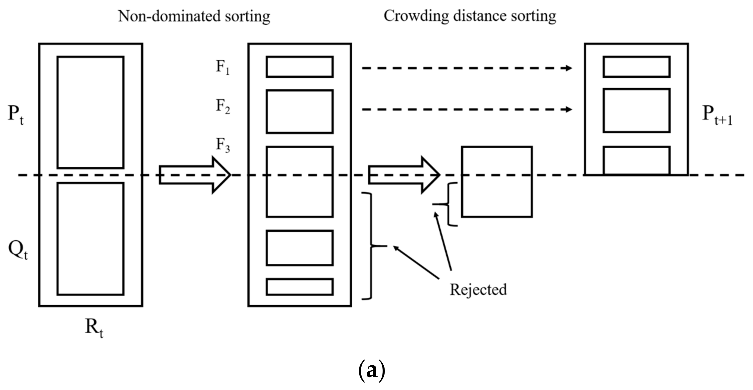
In this paper, we have established the Kriging metamodel of dimensional parameters on the cooling temperature (T) and the cooling capacity (W); multiple established Kriging metamodels collectively act as the target response solver for each iteration of the genetic algorithm. In order to solve the multi-objective optimization problem, the Kriging model optimized by NSGA II based on the Pareto optimal solution is adopted. NSGA-II [24] adopts the elite strategy to expand the sample collection range. Non-dominated sorting is used to compete the parent population with the offspring, and the excellent individuals are retained to the next generation population, which improves the optimization accuracy. At the same time, the method of “crowding distance sorting” is adopted, so that the individual can fully expand to the whole Pareto calculation domain and avoid falling into the local optimal solution.
The crowding algorithm requires that all solutions of the population be arranged in ascending order according to the value of the objective function. For each objective function, first find the boundary solution (the solution corresponding to the maximum and minimum value of the function), and set its distance parameter md value to infinity. The distance parameter values of each solution i are shown in Equation (25).
d m ( i ) = f m ( i + 1 ) f m ( i 1 ) f m max f m min
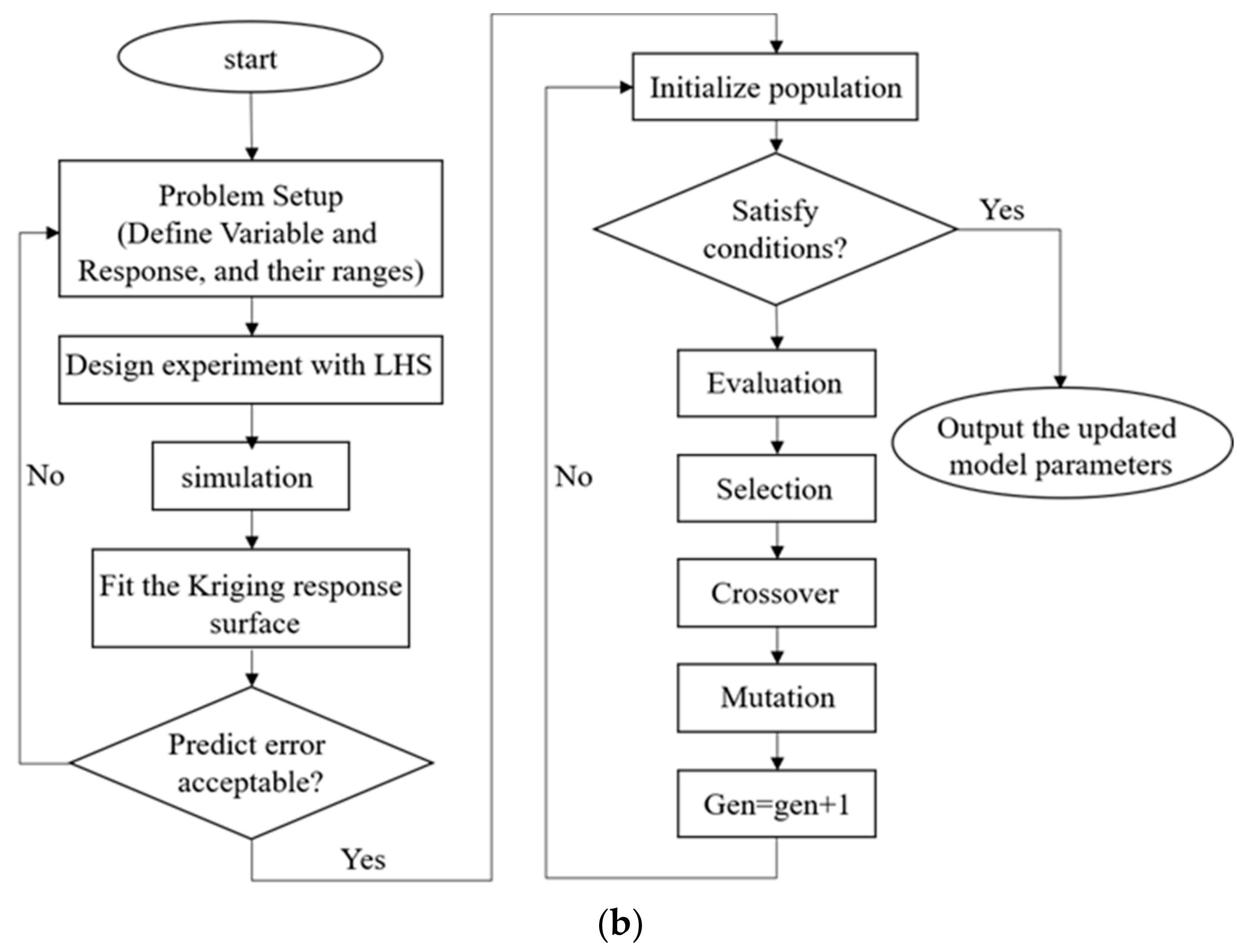
where f m max and f m min are the maximum and minimum values of the mth objective function. The congestion value of individual i is the weighting of all the objective function distance parameters dm. The specific process description of NSGA-II is shown in Figure 2a. The schematic diagram of the optimization iterative process is presented in Figure 2b. The set of Pareto solutions as a result of the iterations is the combined set of optimal values on the multiple Kriging metamodels.

3. Design of Experiments

3.1. Model Validation

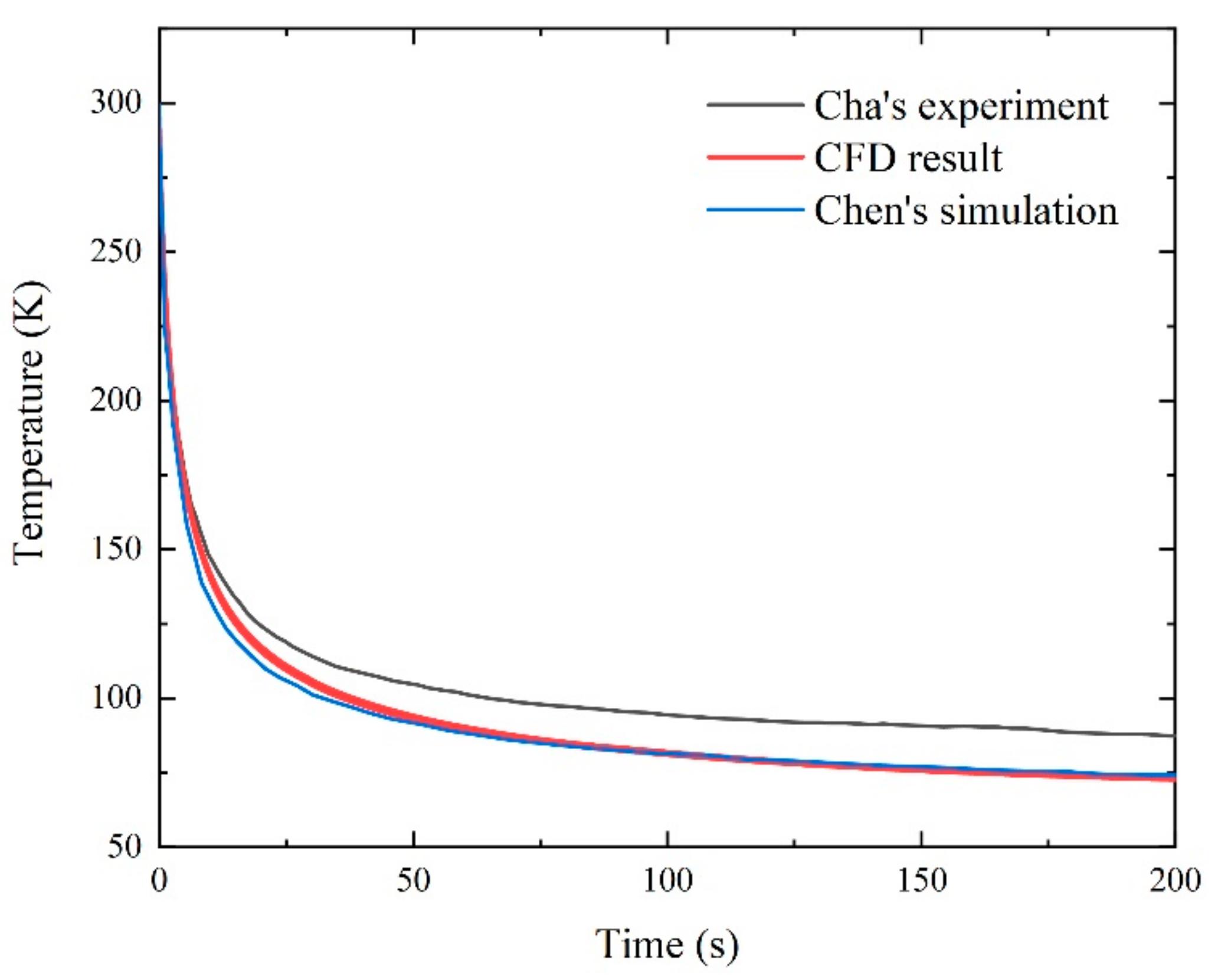
In this section, the validity of the developed CFD model is verified by comparison with Cha’s work [25]. The dimensions of the model are 8 mm (RD), 58 mm (RL), 5 mm (PD) and 60 mm (PL) for the regenerator and pulse tube dimensions, which are consistent with the dimensions of Cha’s experimental setup. Figure 3 presents the contrasting results of the CFD simulation with Cha. The cooling trend of the CFD model is approximately the same as that of Cha’s experiment, and the average temperature of the simulated CHX wall is finally stable at 71 K, which is lower than the experimental result of 87 K. Chen [26] compares his numerical simulation results with Cha’s experimental results and explains the reasons for the difference: the model adopts the laminar flow assumption and the heat balance model, without wall thickness, and the working gas is an ideal gas. In addition, the difference between the ideal and real heat transfer in the regenerator and heat exchanger is also an important reason for the difference in results. The reliability of this paper has been verified, as it is highly consistent with Chen’s simulation.

3.2. Kriging Meta Modeling

Analyzing the effect of variations in the dimensional parameters of the regenerator and the pulse tube on the refrigeration cooling performance is the purpose of this paper; therefore, the factors are identified as the diameter and length of the regenerator (RD and RL) and the diameter and length of the pulse tube (PD and PL), and the response as the cooling temperature (T) and the cooling capacity (W) used to judge the refrigeration performance, in which the W is measured when the wall temperature of CHX is 120 K. The diameter and length range from 4 to 10 mm and 50 to 150 mm, respectively. A Design of Experiment (DOE) was carried out using Latin Hypercube Sampling (LHS) [27] with 26 sample points in the determined factor interval, among which 4 sample points were used for validation, and a CFD model was developed for each sample point, and T and W were obtained by numerical simulation. The Kriging metamodel is developed and solved based on Matlab 2020. Table 2 shows the selected sample points and numerical simulation results.

3.3. Kriging Model Validation

To verify the accuracy of the constructed Kriging model, three sample points were randomly generated as test samples within the interval, using the LHS. Table 3 shows the results of the CFD simulations of the test samples compared to their predicted values in the Kriging model. The maximum error between the CFD results and the predictions for cooling temperature and cooling capacity is 4.85%, with the remaining error values being within 2.5%. T and W can be accurately predicted by the Kriging model within the selected parameter interval.

4. Results and Discussion

4.1. Analysis of Influencing Factors of T and W

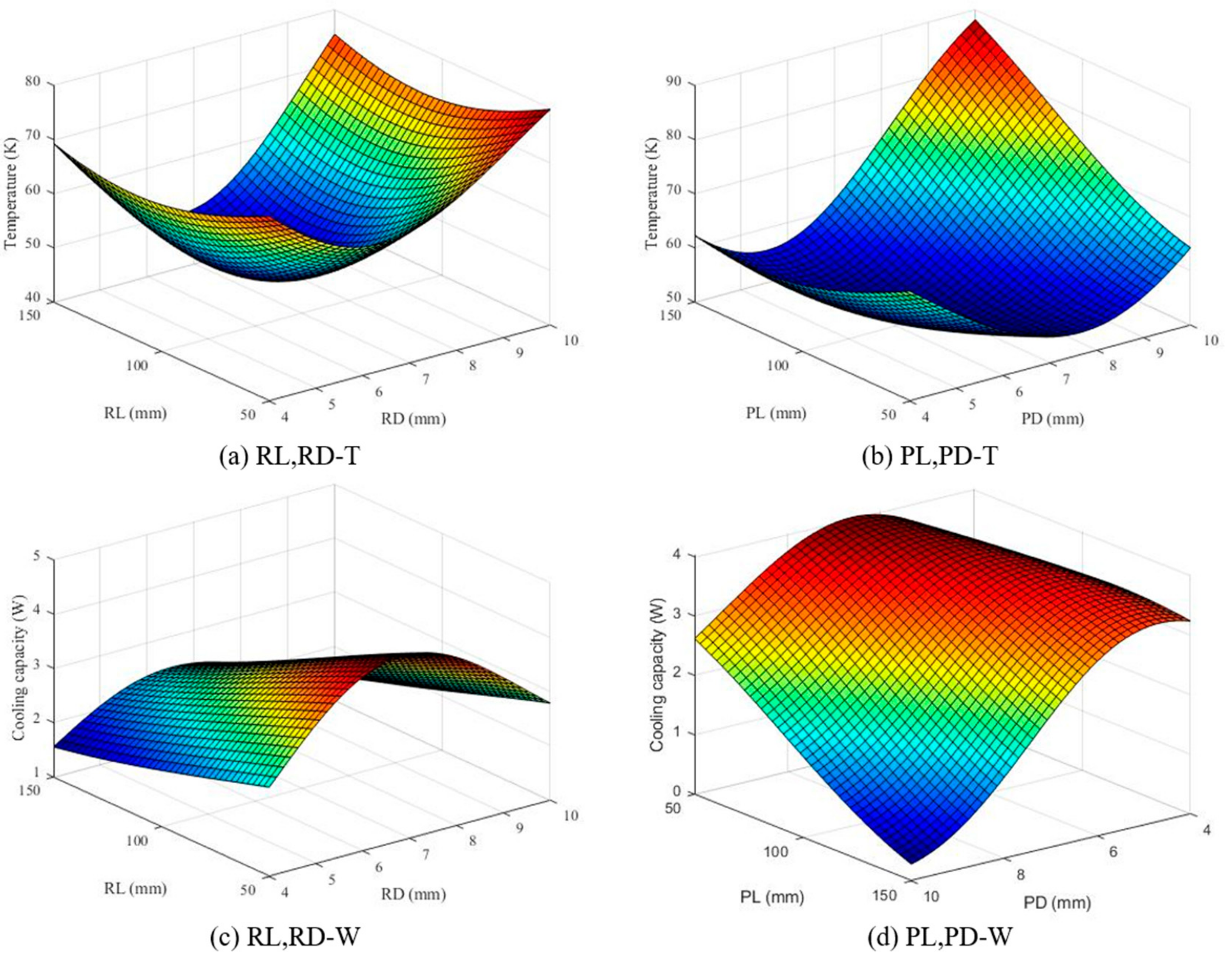
Figure 4a shows the response surface of the regenerator sizes RD and RL with respect to the cooling temperature, where the pulse tube size PD = 6.4 mm and PL = 80 mm. With the increase of RD, the cooling temperature first decreases and then increases. The lowest cooling temperature appears between 6–8 mm in diameter, which changes with the change of RL. With the increase of RL, the cooling temperature also shows a trend of decreasing first and then increasing, and the lowest cooling temperature is reached at RL = 120 mm.
Figure 4b shows the response surface of pulse tube sizes PD and PL with respect to the cooling temperature, where the regenerator size RD = 6.9 mm and RL= 80 mm. With the increase of PD, the cooling temperature first decreases and then increases. There is an optimal PD value to minimize the cooling temperature, and the optimal PD value continues to decrease with the increase of PL. The influence of the PL change on the cooling temperature is greatly affected by PD, showing a completely opposite trend under different PD values. When PD is small, the increase of PL will cause the cooling temperature to drop, while when PD is large, the increase of PL will cause the cooling temperature to rise.
Figure 4c shows the response surface of the regenerator sizes RD and RL with respect to the cooling capacity, where the pulse tube size PD = 6.4 mm and PL = 80 mm. With the increase of RL, the cooling capacity decreases continuously. With the change of RD, the cooling capacity first increases and then decreases. According to the difference of RL, the optimal cooling capacity is between 6–7 mm in diameter.
Figure 4d shows the response surface of the pulse tube sizes PD and PL with respect to the cooling capacity, where the regenerator size RD = 6.9 mm and RL = 80 mm. With the increase of PD, the cooling capacity first increases and then decreases. When PD is different, the influence of PL on the cooling capacity shows different trends. When PD is small, the influence of PL on the cooling capacity is small, and when PD is large, the increase of PL will significantly reduce the cooling capacity.
In Figure 4, PD and PL interact with each other when the dimensional parameters of the pulse tube affect the cooling performance. A larger PD causes a larger dead space at the ends of the pulse tube, deteriorating the cooling performance, which sometimes results in the exact opposite trend of the influence of PL. The working gas in the regenerator has to undergo periodic heat exchange with the packing while transferring as much acoustic power as possible from the hot end to the cold end. A smaller RL or RD is, therefore, not conducive to heat exchange in the regenerator, while a larger RL and RD increase the losses in the regenerator and lead to a deterioration in cooling performance. The four dimensional parameters, therefore, need to be taken into account in order to optimize the optimum size.

4.2. Analysis of NSGA II Optimization Results

NSGA II is used to optimize the two Kriging models constructed for the cooling temperature and the cooling capacity with multiple objectives. If single-objective optimization is used, the two Kriging models need to be optimized separately, and it is not possible to obtain an optimal solution that satisfies both objectives. Equation (26) is the multiple objectives function and constraints for NSGA II, where T ( R D , R L , P D , P L ) and W ( R D , R L , P D , P L ) are constructed Kriging models of T and W, respectively.
{ F i n d   R D , 4 m m R D 10 m m R L , 50 m m R L 150 m m P D , 4 m m P D 10 m m P L , 50 m m P L 150 m m M i n [ T ( R D , R L , P D , P L ) ] M a x [ W ( R D , R L , P D , P L ) ]
NSGA II was run using MATLAB 2020 software, the initial population size was 40, the number of iterations was 200, the probability of variation was set to 0.05, and the crossover probability was 0.8.
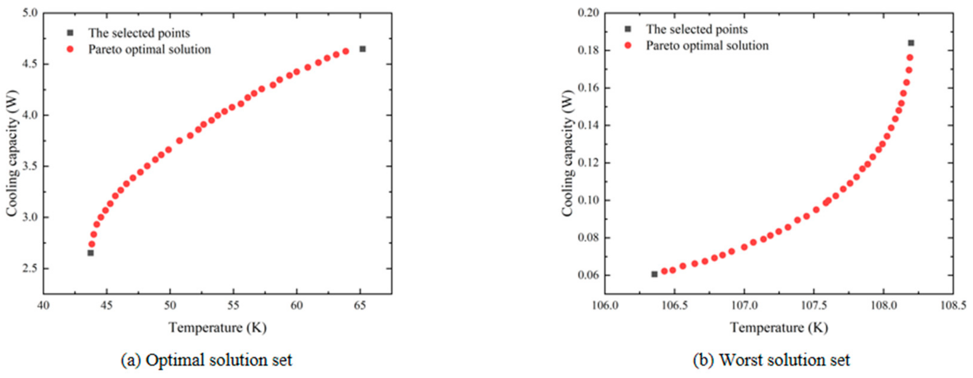
Figure 5a,b are the Pareto optimal solution and the worst solution sets of the constructed Kriging model, respectively. The optimal solution is found to optimize the constructed Kriging metamodel in order to determine the optimal cooling performance and the corresponding dimensional parameters of the pulse tube refrigerator. The worst solution is used to better compare the analysis with the optimal solution and to investigate the mechanism of the effect of the excellent dimensions on the physical quantities of the pulse tube refrigerator. The black square points in Figure 5 are two representative solutions selected from each of the two sets of Pareto fronts solved—solution A1 with the lowest cooling temperature, solution A2 with the highest cooling capacity, solution A3 with the lowest cooling capacity, and solution A4 with the highest cooling temperature—and their dimensional parameters and error comparisons are shown in Table 4. This table shows a maximum difference of 4.59 K in cooling temperature and 0.21 W in cooling capacity between the predicted and simulated values, indicating that the Pareto solution set is highly accurate. The CFD simulation was used to solve for the initial size of the pulsed tube refrigerator (RD = 8 mm, RL = 58 mm, PD = 5 mm, PL = 60 mm), with T being 70.08 K and W being 3.69 W in the results. After optimization, A1 reduces the minimum cooling temperature by 31.24%, and A2 increases the cooling capacity at 120 K by 31.7%. In Section 5, the four solutions are compared and analyzed in detail from the loss of the regenerator and the pulse tube.

5. Analysis of CFD Simulation Results

From the previous optimization results, it is clear that different combinations of regenerator and pulse tube sizes can lead to significant differences in the refrigeration performance of the PTR. Separate analyses for the regenerator and pulse tube are carried out in the subsequent subsections to evaluate the advantages and disadvantages of the refrigeration performance of each Pareto solution from a loss perspective.

5.1. Analysis of Regenerator Losses

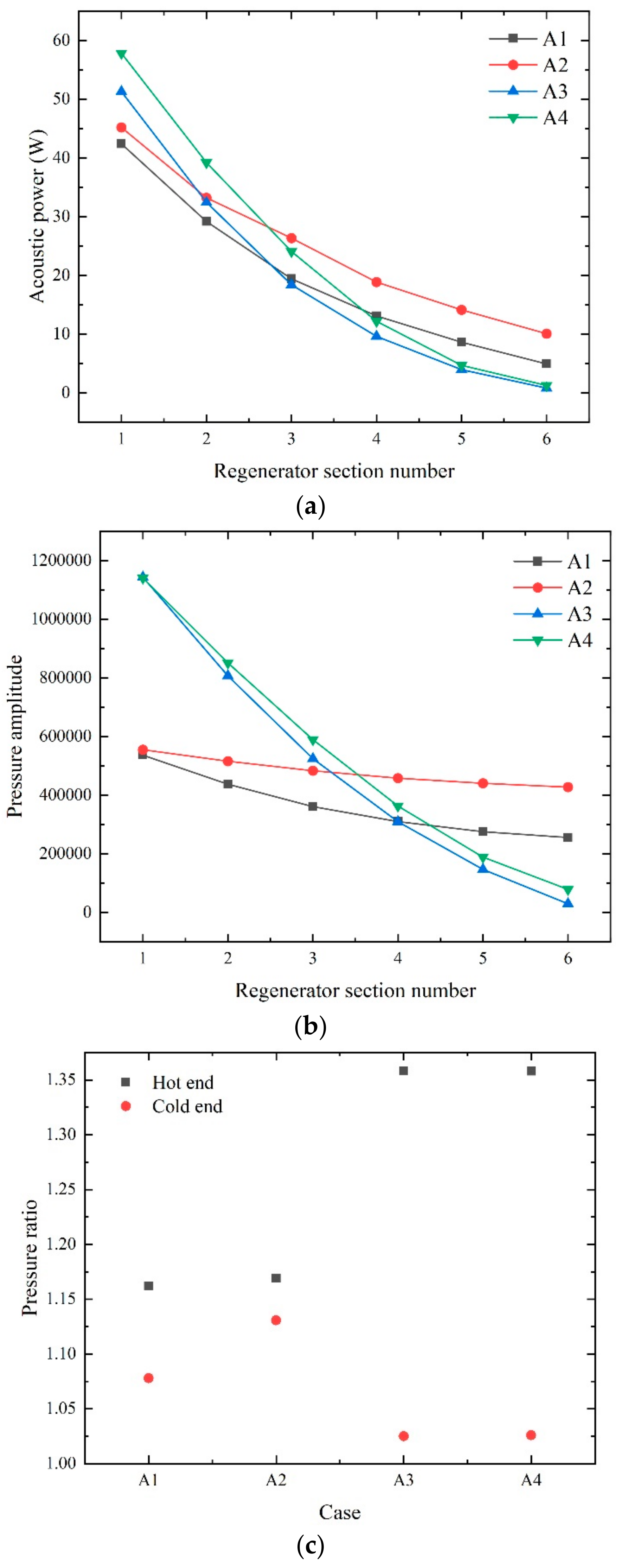
Figure 6a shows the variation of acoustic power in different regenerators along an equidistant cross-section in the axial direction. In the following, the regenerator and pulse tube are divided into 6 radial sections along the axial symmetry axis and numbered 1–6, so as to intuitively observe the change rule of each physical quantity along the axial direction. The change trend of acoustic power in A1 and A2 in the figure is relatively similar. Compared with A3 and A4, the acoustic power in the regenerator inlet section is smaller; the acoustic power in the outlet section is larger; and the loss along the way of acoustic power is 37.49 W and 35.13 W, respectively, while the losses along the way of A3 and A4 are 50.51 W and 56.58 W, respectively. The loss of acoustic power in the regenerator is an important reason for the difference in their refrigeration performance.
According to Equation (1), pressure amplitude is an important factor influencing acoustic power. The change of pressure amplitude can reflect the change trend of pressure drop loss. It can be seen from Figure 6b that the pressure amplitude changes along the axial equidistant section in the regenerator, and the trend is similar to Figure 6a. The working medium gas in the regenerator will exchange heat with the packing under the viscous effect, resulting in resistance loss, causing the pressure drop along the axial direction of the regenerator in the figure. The pressure amplitude of A1 and A2 is significantly smaller than that of A3 and A4, making their acoustic power loss significantly smaller than that of A3 and A4. At the same time, the pressure amplitude drops in A2 and A4 are always smaller than in A1 and A3, respectively, so that the increase in pressure drop loss in the regenerator due to an increase in RL can be clearly observed with little difference in other dimensional parameters.
In order to obtain the desired regenerator cold end pressure ratio and pulse tube enthalpy flow, A3 and A4 with a large pressure drop loss of the regenerator need to provide a larger hot end pressure ratio. Figure 6c shows the distribution of the cross-sectional pressure ratios at the cold and hot ends of the four Case regenerators mentioned above. The presence of pressure drop forces a larger pressure ratio at the hot end to obtain a higher cold end pressure ratio and pulse tube enthalpy flow to improve the cooling performance, which increases the demand on the compressor. Because the same UDF is used to simulate the reciprocating motion of the compressor in this CFD model, there is an upper limit to its performance. Therefore, even if the pressure ratio at the hot end of A3 and A4 rises to around 1.358, the pressure ratio at the cold end still only increases to around 1.025, which is a large gap from A1 and A2, because the ideal enthalpy flow of the pulse tube cannot be obtained, which is an important reason for the poor cooling performance of A3 and A4.

5.2. Analysis of Pulse Tube Losses

Different from the laminar flow in the regenerator, the velocity of the working medium gas in the pulse tube is fast, which is easy to develop into vortex. At the same time, the radial difference of the axial velocity caused by the existence of the boundary layer will form a secondary flow in the pulse tube. The complex flow of these working medium gases will restrict the performance of the refrigerator.
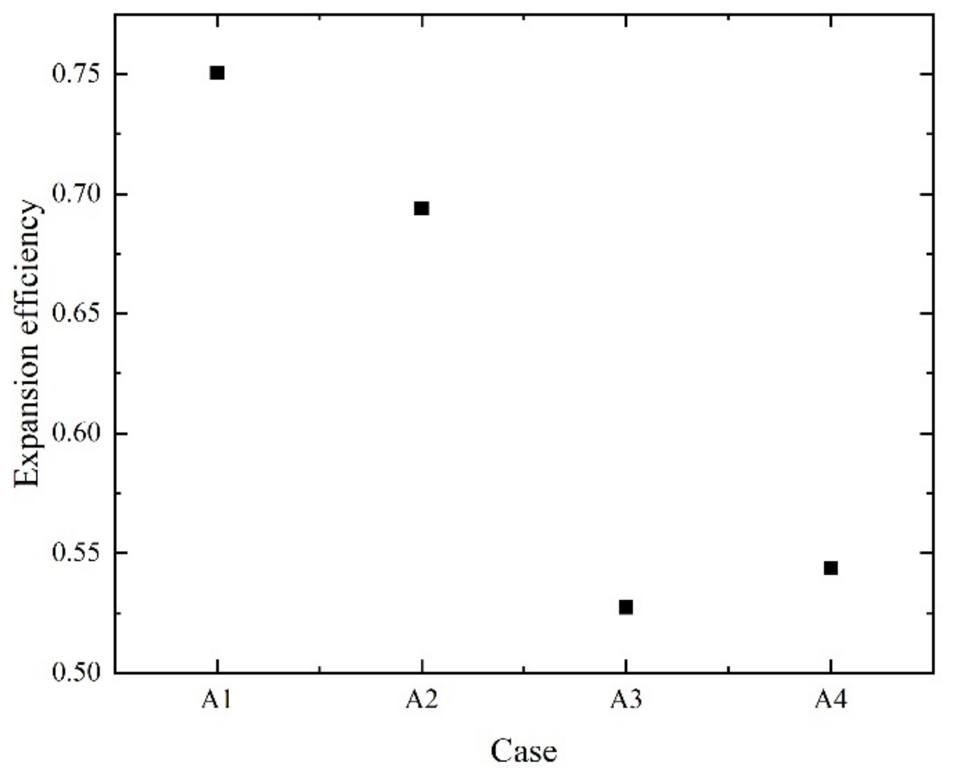
The expansion efficiency is usually used to evaluate the loss in the pulse tube. Figure 7 calculates the expansion efficiency of the pulse tube of 4 Cases, in which the expansion efficiency of A1 and A2 are 0.75 and 0.69, respectively, while the expansion efficiency of A3 and A4 are significantly lower than the former, which are 0.53 and 0.54, respectively, indicating that the loss of working medium gas in the pulse tube is also an important factor causing the difference in refrigeration performance.
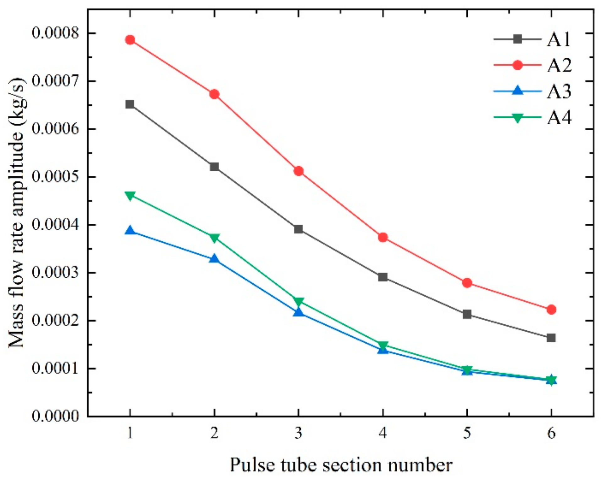
Figure 8 shows the distribution of the mass flow rate amplitude in the pulse tube along the axial equidistant section. A1–A4 all showed a trend in which the amplitude of the mass flow rate gradually decreased along the axial direction. At the same time, the mass flow rate amplitude of A3 and A4 is significantly smaller than that of A1 and A2, and the difference is more obvious at the cold end of the pulse tube. The amplitude of A1 is 227.53% and 215.99% higher than that of A3 and A4, respectively, and the amplitude of A2 is 298.3% and 283.17% higher than that of A3 and A4, respectively, which will lead to a significant reduction in the fluid oscillation intensity in the pulse tube, especially at the cold end of the pulse tube, which is not conducive to refrigeration.
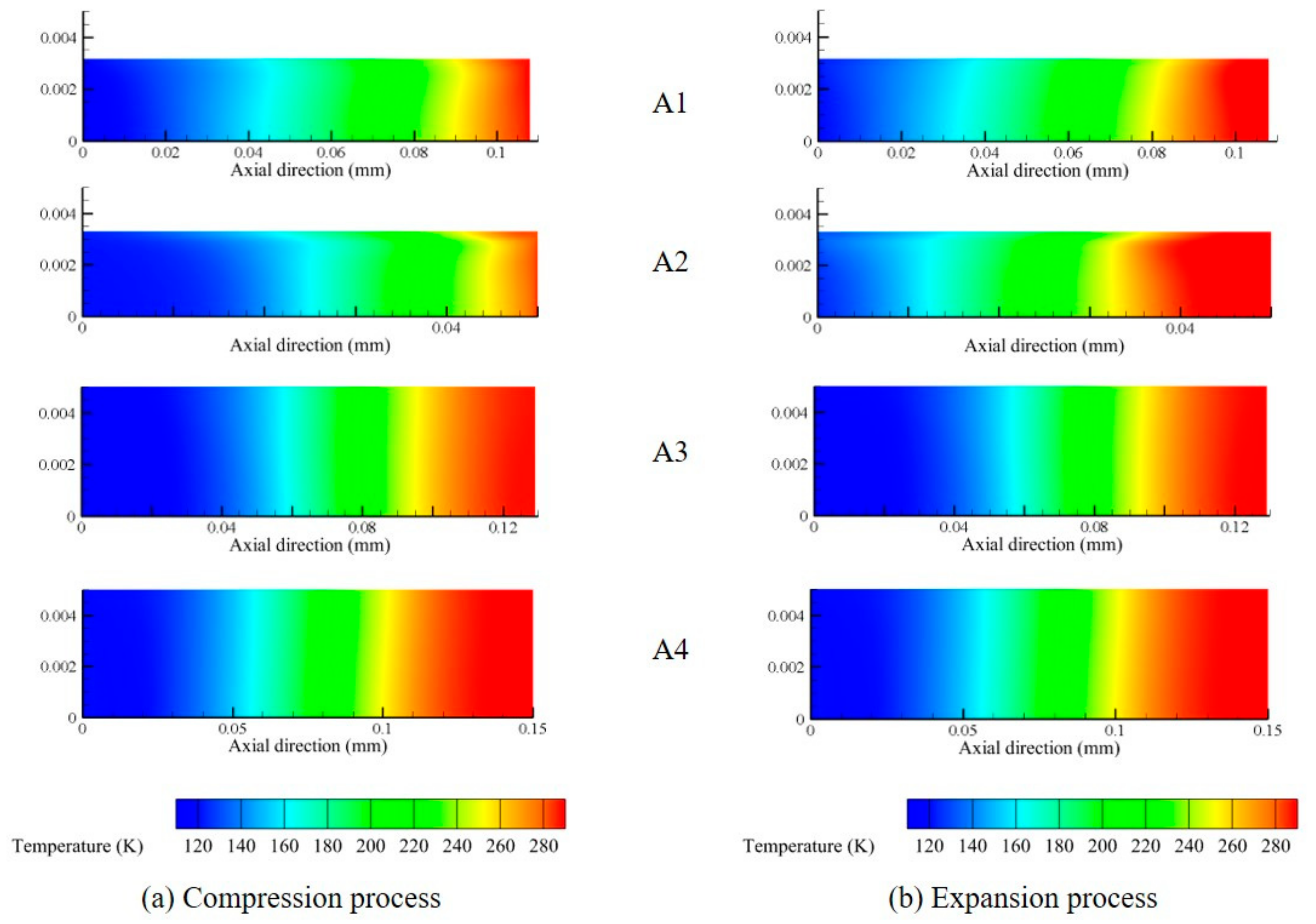
The distribution of the temperature field in the vasculature and the change of the gas piston can be observed to further verify the previous inference. Figure 9 shows the temperature contours of the four Cases after reaching steady state. Figure 9a shows the temperature distribution when the compression process ends and the expansion state is about to begin in a cycle, and Figure 9b shows the temperature distribution when the expansion process ends and the compression state is about to begin in a cycle. These two moments have been chosen to give a good reflection of the movement of the gas piston. A1 and A2 can observe the obvious movement process of the gas piston, and the reciprocating motion of the gas piston of A2 is more intense, while the reciprocating motion of the gas piston of A3 and A4 is very weak, which cannot effectively develop its refrigeration performance. This is the same as the variation trend of the amplitude of the mass flow rate in the previous article, which can better confirm the previous conclusion. There is a radial temperature gradient in A1 and A2 near the wall of the pulse tube, which is greater in A2 than in A1, as can be seen from the temperature contours. A3 and A4 have a relatively straight isotherm inside, with no significant radial temperature gradient. The radial temperature gradient in the pulse tube is mainly caused by the viscous dissipation between the boundary layer and the wall of the pulse tube, and because of the presence of the boundary layer, A1 and A2 have a significant radial velocity gradient at the wall. This can be further analyzed by observing the flow field and vortex volumes.
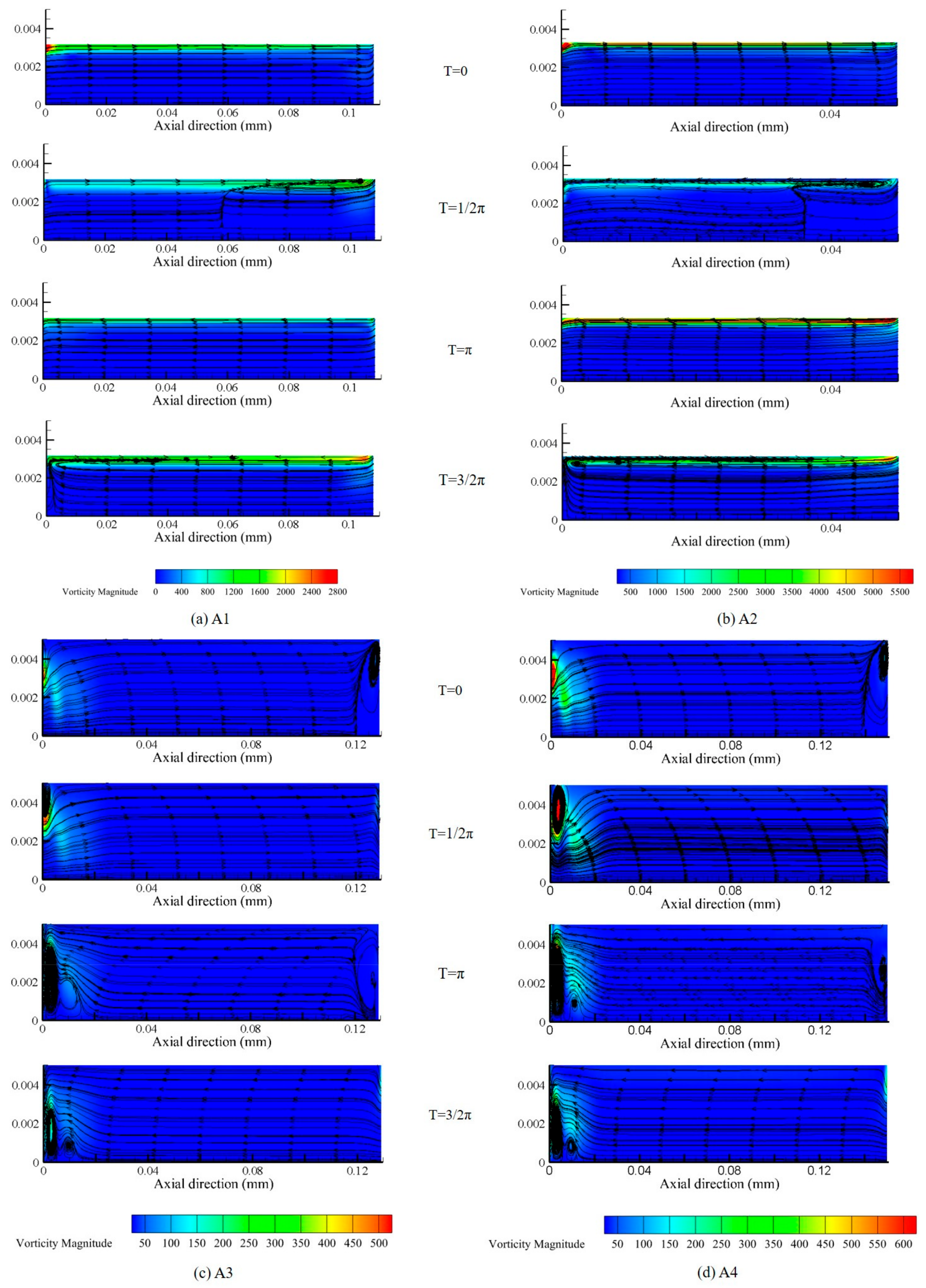
Figure 10 shows the distribution of the flow field and vorticity at four moments in the same cycle of the pulse tube when the four Cases reach steady state. The distribution of the vortex fields in A1 and A2 is similar, with the vortices mainly located close to the wall of the pulse tube and developing axially with the compression and expansion process, mainly due to the radial temperature gradient caused by the viscous effect of the boundary layer in A1 and A2, which leads to the formation of the Rayleigh flow. As the radial temperature gradient is greater in A2, the vortex of A2 occupies more volume in the pulse tube, and its corresponding vortex value is significantly higher than that of A1, thus further confirming that the pulse tube loss is greater in A2 than in A1, resulting in a lower expansion efficiency in A2 than in A1. It can be seen that the vortex fields of A3 and A4 are approximately the same, as the pulse tube diameters of A3 and A4 are both 10 mm, while the diameters of the CHX and WHX connected to them are 6 mm and 8 mm, respectively. This radial difference in size can lead to a larger dead volume at the inlet and outlet ends of the pulse tube, and fully developed vortices are found in both Figure 10c,d in the above-mentioned areas. In addition to the significant gradient in mass flow rate between the cases, the vortex generation conditions are also an important reason for the difference. As can be seen from Figure 7, the dead volume of the pulse tube has a more significant effect on the efficiency than the dissipation at the boundary layer.

6. Conclusions

This paper proposed an approach of combining the Kriging metamodel and genetic algorithms for the optimal design of a pulse tube refrigerator. Conclusions can be drawn as follows:
(I)
The two Kriging models established with four dimensional parameters have been verified to be highly reliable. The results show that the established Kriging model presents a prediction error of about 2.5%. Therefore, replacing the CFD model with it and using it for model updates can significantly improve the iterative efficiency.
(II)
Combining the Kriging method modeling and NSGA II can solve multi-objective optimization problems. In this paper, the Pareto front solution with the optimal and worst cooling temperature and cooling capacity is solved, and a 31.24% drop in the minimum cooling temperature and a 31.7% increase in the cooling capacity at 120 K are achieved after optimization.
(III)
A1–A4 are analyzed from the perspective of the regenerator and the pulse tube, respectively. The pressure drop loss at the regenerator is an important reason for the deterioration of the refrigeration performance, the unreasonable pulse tube structure will cause a large dead space, and the existence of eddy viscosity will seriously restrict the expansion efficiency of the pulse tube.
(IV)
After verification, the Kriging model combined with NSGA-II optimization is highly feasible in the field of pulse tube research, and the current study provides a scientific and efficient design method for miniature cryogenic refrigerators.

Author Contributions

Writing–review & editing, H.Z.; Supervision, W.S., Z.C. and C.Z. All authors have read and agreed to the published version of the manuscript.

Funding

This research was funded by China Postdoctoral Fund Program (2022M711955), Taishan Scholar Project (tsqn202103142), Youth Fund of Shandong Natural Science Foundation (ZR2021QE182) and Natural Science Foundation of Shandong Province (ZR2020ME192).

Data Availability Statement

Data is contained within the article.

Conflicts of Interest

The authors declare no conflict of interest.

References

  1. Gifford, W.E.; Longsworth, R.C. Pulse-Tube Refrigeration. Trans. ASME J. Eng. Ind. 1964, 86, 264–268. [Google Scholar] [CrossRef]
  2. Radebaugh, R.; Louie, B.; Smith, D.R. A comparison of three types of pulse tube refrigerators—New methods for reaching 60 K. In Advances in Cryogenic Engineering; Springer US: New York City, NY, USA, 1986. [Google Scholar]
  3. Shaowei, Z.; Peiyi, W.; Zhongqi, C. Double inlet pulse tube refrigerators: An important improvement. Cryogenics 1990, 30, 514–520. [Google Scholar] [CrossRef]
  4. Ju, Y.L.; Wang, C.; Zhou, Y. Dynamic experimental investigation of a multi-bypass pulse tube refrigerator. J. Eng. Thermophys. 1997, 37, 357–361. [Google Scholar] [CrossRef]
  5. Kanaoki, K.I.; Watanabe, N.; Kanazawa, Y. A miniature pulse tube refrigerator for temperatures below 100K. Cryogenics 1994, 34, 167–170. [Google Scholar] [CrossRef]
  6. Bao, D.; Tan, J.; Zhang, L.; Gao, Z.; Zhao, Y.; Dang, H. A two-dimensional model of regenerator with mixed matrices and experimental verifications for improving the single-stage Stirling-type pulse tube cryocooler. Appl. Therm. Eng. 2017, 123, 1278–1290. [Google Scholar] [CrossRef]
  7. Dang, H.; Zhao, Y. CFD modeling and experimental verification of a single-stage coaxial Stirling-type pulse tube cryocooler without either double-inlet or multi-bypass operating at 30–35 K using mixed stainless steel mesh regenerator matrices. Cryogenics 2016, 78, 40–50. [Google Scholar] [CrossRef]
  8. Wu, W.; Cui, X.; Liu, S.; Jiang, Z.; Song, J.; Wu, Y. Cooling performance improvement of a two-stage pulse tube cryocooler with Er-plated screen as regenerator material. Int. J. Refrig. 2021, 131, 615–622. [Google Scholar] [CrossRef]
  9. Liu, X.; Chen, C.; Huang, Q.; Wang, S.; Hou, Y.; Chen, L. Modeling of heat transfer and oscillating flow in the regenerator of a pulse tube cryocooler operating at 50 Hz. Appl. Sci. 2017, 7, 553. [Google Scholar] [CrossRef] [Green Version]
  10. Rawlins, W.; Radebaugh, R.; Bradley, P.E.; Timmerhaus, K.D. Energy Flows in an Orifice Pulse Tube Refrigerator. Adv. Cryog. Eng. 1994, 39, 1449–1456. [Google Scholar]
  11. Swift, G.W. Analysis and performance of a large thermoacoustic engine. J. Acoust. Soc. Am. 1992, 92, 1551–1563. [Google Scholar] [CrossRef]
  12. Gu, C.; Zhou, Y.; Wang, J.; Ji, W.; Zhou, Q. CFD analysis of nonlinear processes in pulse tube refrigerators: Streaming induced by vortices. Int. J. Heat Mass Transf. 2012, 55, 7410–7418. [Google Scholar] [CrossRef]
  13. Zhao, Y.; Yu, G.; Tan, J.; Mao, X.; Li, J.; Zha, R.; Li, N.; Dang, H. CFD modeling and experimental verification of oscillating flow and heat transfer processes in the micro coaxial Stirling-type pulse tube cryocooler operating at 90–170 Hz. Cryogenics 2018, 90, 30–40. [Google Scholar] [CrossRef]
  14. Ashwin, T.R.; Narasimham, G.; Jacob, S. CFD analysis of high frequency miniature pulse tube refrigerators for space applications with thermal non-equilibrium model. Appl. Therm. Eng. 2010, 30, 152–166. [Google Scholar] [CrossRef] [Green Version]
  15. Antao, D.S.; Farouk, B. Numerical simulations of transport processes in a pulse tube cryocooler: Effects of taper angle. Int. J. Heat Mass Transf. 2011, 54, 4611–4620. [Google Scholar] [CrossRef]
  16. Dai, Q.; Chen, Y.; Yang, L. CFD investigation on characteristics of oscillating flow and heat transfer in 3D pulse tube. Int. J. Heat Mass Transf. 2015, 84, 401–408. [Google Scholar] [CrossRef]
  17. Rout, S.K.; Choudhury, B.K.; Sahoo, R.K.; Sarangi, S.K. Multi-objective parametric optimization of Inertance type pulse tube refrigerator using response surface methodology and non-dominated sorting genetic algorithm. Cryogenics 2014, 62, 71–83. [Google Scholar] [CrossRef]
  18. Panda, D.; Satapathy, A.K.; Sarangi, S.K. Thermo-hydrodynamic analysis and optimal design of a GM cycle cryorefrigerator using response surface methodology and particle swarm optimization. Sci. Technol. Built Environ. 2019, 25, 1467–1481. [Google Scholar] [CrossRef]
  19. Keshtegar, B.; Mert, C.; Kisi, O. Comparison of four heuristic regression techniques in solar radiation modeling: Kriging method vs RSM, MARS and M5 model tree. Renew. Sustain. Energy Rev. 2018, 81 Pt 1, 330–341. [Google Scholar] [CrossRef]
  20. Sun, Z.; Wang, J.; Li, R.; Tong, C. LIF: A new Kriging based learning function and its application to structural reliability analysis. Reliab. Eng. Syst. Saf. 2017, 157, 152–165. [Google Scholar] [CrossRef]
  21. Zhao, J.P.; Wang, J.T.; Wang, C.J. Frequency response function-based model updating using Kriging model. Mech. Syst. Signal Process. 2017, 87, 218–228. [Google Scholar]
  22. Zheng, C.; Zhao, H.; Zhou, Z.; Geng, Z.; Cui, Z. Investigation on thermal model updating of Alpha Magnetic Spectrometer in orbit based on Kriging meta-modeling. Nucl. Instrum. Methods Phys. Res. Sect. A Accel. Spectrometers Detect. Assoc. Equip. 2022, 1031, 166581. [Google Scholar] [CrossRef]
  23. Chen, S.; Shi, T.; Wang, D.; Chen, J. Multi-objective optimization of the vehicle ride comfort based on Kriging approximate model and NSGA-II. J. Mech. Sci. Technol. 2015, 29, 1007–1018. [Google Scholar] [CrossRef]
  24. Deb, K.; Agrawal, S.; Pratap, A.; Meyarivan, T. A fast elitist non-dominated sorting genetic algorithm for multi-objective optimization: NSGA-II. Lect. Notes Comput. Sci. 2000, 1917, 849–858. [Google Scholar]
  25. Cha, J.S.; Ghiaasiaan, S.M.; Desai, P.V.; Harvey, J.P.; Kirkconnell, C.S. Multi-dimensional flow effects in pulse tube refrigerators. Cryogenics 2006, 46, 658–665. [Google Scholar] [CrossRef]
  26. Chen, L.; Zhang, Y.; Luo, E.; Li, T.; Wei, X. CFD analysis of thermodynamic cycles in a pulse tube refrigerator. Cryogenics 2010, 50, 743–749. [Google Scholar] [CrossRef] [Green Version]
  27. Zhang, F.; Cheng, L.; Wu, M.; Xu, X.; Wang, P.; Liu, Z. Performance analysis of two-stage thermoelectric generator model based on Latin hypercube sampling. Energy Convers. Manag. 2020, 221, 113159. [Google Scholar] [CrossRef]
Figure 1. Structure diagram of pulse tube refrigerator.
Energies 16 02736 g001
Figure 2. (a) Main process of NSGA-II. (b) Flow chart for building and optimizing the Kriging model.
Energies 16 02736 g002aEnergies 16 02736 g002b
Figure 3. Comparison of cooling curve of CHX wall.
Energies 16 02736 g003
Figure 4. Three-dimensional projection of the Kriging model.
Energies 16 02736 g004
Figure 5. NSGA II multi-objective optimization of Pareto solution sets.
Energies 16 02736 g005
Figure 6. (a) Acoustic power distribution along the axially equidistant section of the regenerator. (b) Pressure amplitude distribution along the axially equidistant section of the regenerator. (c) Hot and cold end pressure ratio of the regenerator.
Energies 16 02736 g006
Figure 7. Pulse tube expansion efficiency.
Energies 16 02736 g007
Figure 8. Mass flow rate amplitude distribution along the axially equidistant section of the pulse tube.
Energies 16 02736 g008
Figure 9. Distribution of pulse tube temperature contours.
Energies 16 02736 g009
Figure 10. Distribution of streamtraces and vorticity magnitude in the pulse tube.
Energies 16 02736 g010
Table 1. Dimension parameters, boundary conditions and area type settings of various parts of the pulse tube refrigerator.
ComponentNo.Diameter (mm)Length (mm)Wall MaterialBoundary Condition
CompressorA19.087.5stainless steelAdiabatic
Transfer tubeB3.1101stainless steelAdiabatic
AftercoolerC820Cu293 K
RegeneratorD//stainless steelAdiabatic
Cold heat exchanger
(CHX)
E65.7CuAdiabatic/120 K
Pulse tubeF//CuAdiabatic
Warm heat exchanger
(WHX)
G810Cu293 K
Inertance tubeH0.85684stainless steelAdiabatic
ReservoirI26130stainless steelAdiabatic
Table 2. LHS sample set and numerical simulation results.
No.RD (mm)RL (mm)PD (mm)PL (mm)T (K)W (W)
15.5065.366.98116.0164.492.82
24.08106.028.96105.4792.230.65
39.05118.996.5251.6370.232.35
49.91112.274.15133.2668.551.92
58.5853.866.00140.6565.213.05
69.4856.587.29127.1577.471.92
76.00145.694.8183.9259.002.54
84.58127.487.60123.7670.751.10
97.35132.604.95149.8151.712.57
106.8264.478.5268.1760.073.35
116.50140.837.5661.7150.912.45
125.2576.628.4196.3468.312.01
138.41104.625.2659.6062.582.63
147.27138.955.5074.1653.302.57
156.5281.359.8175.7067.252.06
169.1799.146.50100.5059.732.35
178.0093.509.4385.5466.851.76
188.0070.618.00113.6568.652.15
195.03121.074.5391.9362.022.51
204.6187.549.36135.9294.230.52
218.00585.006070.083.69
229.2854.739.9051.579.282.18
238.00101.388.6465.2659.602.54
Table 3. Test sample results and errors.
No. Design ParametersResponse Values
RD (mm)RL (mm)PD (mm)PL (mm) KrigingCFDError
15.2262.778.689.9T(K)70.4871.000.74%
W(W)2.232.172.82%
28.64141.565.2122.59T(K)54.6153.332.40%
W(W)2.082.022.79%
36.8121.494.74132.96T(K)51.6150.492.21%
W(W)2.853.004.85%
Table 4. Results and errors of the selected Pareto solutions.
No. Design ParametersResponse Values
RD (mm)RL (mm)PD (mm)PL (mm) KrigingCFDError
A17.021226.34107.92T(K)43.7348.194.46
W(W)2.652.640.01
A26.8506.650T(K)65.262.772.43
W(W)4.654.860.21
A3415010129.19T(K)106.36107.23.0.87
W(W)0.060.210.15
A44114.9410150T(K)108.2112.794.59
W(W)0.1840.050.134
Disclaimer/Publisher’s Note: The statements, opinions and data contained in all publications are solely those of the individual author(s) and contributor(s) and not of MDPI and/or the editor(s). MDPI and/or the editor(s) disclaim responsibility for any injury to people or property resulting from any ideas, methods, instructions or products referred to in the content.