Statistical Analysis of Electric Vehicle Charging Based on AC Slow Chargers

Abstract

Regarding DC fast chargers, various studies, such as the charge scheduling, have been conducted. On the other hand, research on AC slow chargers has rarely been conducted due to the predictable and simple usage pattern. Despite the long charging times of AC slow chargers, which use the existing electric outlets with relatively low supplied power, these chargers are suitable for daily home charging of electric vehicles (EVs) during the night. Due to their low installation costs, they are likely to be the dominant type of charging equipment. In this paper, the EV charging process based on AC slow chargers, which supply a maximum power of 3 kW from an AC 220 V outlet, is analyzed by constructing a simple charging model. The charging time and fees are statistically derived and investigated. Furthermore, power load curves for charging EVs with the 3 kW charger are observed. From the statistical analyses, we conclude that daily charging of EVs can be an appropriate scenario in using the AC slow chargers, and the power load can be spread without employing any demand response schemes.

1. Introduction

Climate change poses a serious threat to a sustainable society. The International Panel on Climate Change (IPCC) states that these changes are mainly caused by the prolonged use of fossil fuels and the resulting emission of greenhouse gases. To mitigate this threat to human civilization, IPCC has proposed that major countries around the world achieve carbon neutrality by 2050, and action plans for carbon neutrality in various industries, such as energy, buildings, and agriculture, have been proposed [1]. Electric vehicles (EVs) replacing fossil fuel vehicles are also one of the key measures to practice carbon neutrality in the transport sector [2]. The supply of EVs has increased significantly in recent years as a result of major automakers releasing various EVs and consumers’ acceptance of EVs improving. If this trend continues, EVs are expected to account for 54% of new car sales and 33% of global vehicles by 2040 [3]. Along with the spread of EVs, the supply of EV chargers should also be carried out simultaneously. By 2040, it is estimated that over 309 million chargers will be needed globally, including 270 million home chargers, 24 million public chargers, 12 million chargers at work, and 400 chargers for buses and trucks [4].

According to the Society of Automobile Engineers (SAE), EV chargers connected to the grid are categorized into AC and DC levels, as summarized in

Table 1. EV charging levels based on J1772 of SAE (North America).

SAE J1772		Voltage (V)	Current (A)	Power (kW)	Phase
AC	Level 1 (L1)	120	≤16 (12)	≤1.92	1
	Level 2 (L2)	240	≤80 (32)	≤19.2	1
DC		200–600	≤400	≤240

(SAE J1772) [5,6,7]. AC chargers use the on-board-chargers (OBCs), which convert AC power to DC power and charge the battery, require long charging times with low supplying power and are suitable for home or workplace use. Three-phase AC chargers with increased power outputs (>20 kW) are also available (SAE J3068). DC fast chargers (DCFCs), on the other hand, directly supply DC power to EVs, can perform fast charging with high power outputs, and are typically used in situations where quick charging is needed, such as on city roads or highways [8]. In IEC 69196, the EV chargers are classified based on charging speed and charger equipment functions, as shown in

Table 2. EV charging modes based on IEC 69196 (Europe).

IEC 69196 Mode	Speed	Features
Mode 1	Slow	Regular electrical socket (1 or 3 phases)
Mode 2	Slow	Regular socket/EV protection
Mode 3	Slow or fast	EV multi-pin socket/control and protection
Mode 4	Fast	Specific charger technology (CHAdeMO)

. In South Korea, EV chargers can be classified based on the maximum supplying power, as summarized in

Table 3. EV charging classes (South Korea).

Charging Class	Voltage (V)	Current (A)	Power (kW)	Category
Class 3 kW	AC 220	≤16	≤3	AC L2/Mode 1 or 2
Class 7–11 kW	AC 220	≤ 32 or 50	≤7 or 11	AC L2/Mode 1 or 2
Class 50–100 kW	DC		≤150	Mode 3 or 4

. As shown in Table 1, fast chargers use DC power from specific charging equipment, while slow chargers use 110 V or 220 V AC power.

It is expected that 87.4% of the global charger demand in 2040 will come from households, and these EV users will prefer to charge their EVs at home after work. This means that most EV charging equipment will consist of AC slow chargers. The AC Level 1 and Class 3 kW chargers can utilize the existing electrical outlets without additional wiring work, which has the advantage of reducing construction costs significantly. Among slow chargers, the AC Level 1 charger is 50% cheaper than the AC Level 2 charger. Although the AC Level 2 charger is less expensive than a DCFC, it is still a financial burden to purchase it personally. Therefore, the AC Level 1 chargers have the advantage of being more widely installed, particularly in household parking lots, due to their low cost.

When operating an EV, the time required to charge the EV is an important factor. Although AC slow chargers have relatively longer charging times compared to DCFC, they provide the benefit of being able to charge at home after returning from a drive. Unlike gasoline-powered vehicles, which need to be refueled at a gas station, EV drivers can use slow AC chargers to charge their vehicles overnight at home. Therefore, slow chargers can be a good choice for charging EVs at home instead of expensive DCFC. In addition, there may be issues with obtaining consent for charger installation in shared parking spaces, particularly in apartment complexes. For the case of installing chargers in parking lots used by a large number of residents, obtaining consent from non-EV drivers to restrict certain parking spaces for EV charging is not easy because non-EVs are prohibited from using those spaces. However, compared to the case of DCFCs, AC slow chargers do not pose such restrictions on parking for non-EVs, making it easier to gain consent from residents.

Studies on the impact of the electrical grid system related to the dissemination of EVs are divided into two main topics. The first topic is related to balancing power usage in response to the large-scale adoption of EVs. It is expected that the peak load burden on the power system will increase with the widespread use of EVs, as it is projected that around 30% of all cars will be replaced by EVs by 2040. Therefore, to address the potential strain on the electrical grid system caused by the widespread use of EVs, various demand response (DR) studies have been conducted regarding EV charging stations [9,10,11]. Most research in DR highlights the advantage of the ease of participation for EV users, while some studies suggest that the burden on the power system may increase if a large number of EV users participate in the DR program at the same time [12]. The second topic is about the impact of EV charging on the power distribution network with regards to voltage management, power quality, and the deterioration of distribution transformers, and it is of concern to power distribution companies [13,14,15,16,17,18].

In this paper, we analyze the AC slow charger of Class 3 kW, which can be installed at low costs by using existing AC 220 V outlets, especially in residential areas, as shown in Table 3. Note that this charging class has the properties of AC Level 1 and Modes 1 and 2 of Table 1 and Table 2. A simple charging model for the slow charger is first developed and the charging times are calculated based on the fuel efficiencies of EVs that are sold a lot in South Korea. Although the charging time is long, the daily EV charging scenario is useful enough for commuter EV drivers. Based on the charging model and several dynamic rate plans for EV charging, the charging fee is formulated and statistically analyzed. The power load for charging EVs with AC slow chargers is also statistically analyzed by observing the peak power load. Due to the long charging time, the power load can be spread without employing any special schemes, such as DR, and does not affect the availability of the distributed capacity of the grid too much, where various energy sources, such as the renewal energies, are considered.

This paper is organized in the following way. In Section 2, we construct a simple charging model for EVs. The statistical experiments for the charging model are then conducted in Section 3. In Section 4, discussions on the modeling and charging experiments are shown. The conclusion is then stated in the last section.

2. EV Charging Model

In this section, we propose a model for AC slow charging of EV batteries corresponding to Class 3 kW and Class 7–11 kW. This statistical model considers one-day charging of a vehicle, and other characteristics according to weekdays and weekends, seasons, and geographical regions can be extended based on a composite source model.

2.1. EV Charging Time

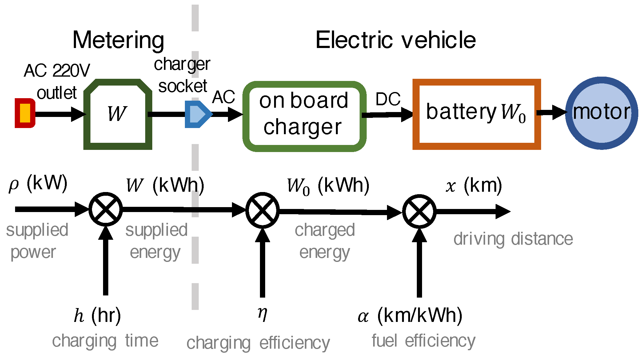
Let $W_0$ (kWh) denote the amount of energy charged in the battery and W (kWh) denote the energy to be supplied. The supplied energy W, which is metered in a metering device, as shown in Figure 1, serves as a basis for calculating electricity fees. $W_0$ is then defined as

$$\begin{array}{c}\hfill W_0:=\eta W\left(\mathrm{k}\mathrm{W}\mathrm{h}\right),\end{array}$$

(1)

where a positive constant $\eta$ represents the charging efficiency that considers both the charger and the battery and is less than 1. According to the 2022 data from the Korea Energy Agency (KEA), for the cases of the 100 kW-class DCFC, the charging efficiency for the charger alone is approximately 95%, and it is planned to increase to 98% in the future. In addition, the battery also has its own efficiency. Slow chargers, such as Class 3 kW and Class 7–11 kW, usually have a higher charging efficiency than fast chargers. Hence, in the statistical analysis, we set the efficiency as $\eta =95\%$. In the case of Class 3 kW, the metering device generally receives power from the conventional AC 220 V outlet and supplies energy to EV through a connector, such as the DC combo, as shown in Figure 1. A wireless charging system can also be considered for slow chargers [19].

In South Korea, there is a performance measure for EVs called the government-approved electric-vehicle fuel efficiency. This measure is divided into two parts for urban and high-speed driving conditions, similar to the fuel efficiency for internal combustion engine vehicles, and there is also a combined fuel efficiency that takes into account both parts. As of September 2022, the latest Hyundai Ioniq 6 has the best-combined fuel efficiency of 6.2 km/kWh in South Korea.

In general, EVs have higher fuel efficiency in urban areas compared to high-speed driving conditions. For instance, the Hyundai Ioniq 6 has fuel efficiencies of 6.8 km/kWh in urban areas and 5.5 km/kWh in high-speed driving conditions.

Let us denote the fuel efficiency of an EV as $\alpha$ (km/kWh). Then, as illustrated in Figure 1, the daily driving distance x that can be derived with the charged energy $W_0$ is given as

$$\begin{array}{c}\hfill x=\alpha W_0\left(\mathrm{k}\mathrm{m}\right).\end{array}$$

(2)

Here, $\alpha$ represents a discharging efficiency. From (1) and (2), the supplied energy W can be written as $W=x/\alpha \eta$, a function of the driving distance x. Therefore, the longer the distance traveled, the more energy required. According to a survey conducted by the Korea Electric Power Research Institute (KEPRI) in 2022, the average daily driving distance of approximately 10,000 households with EVs was 60.9 km, which is higher than the average of 39.6 km of conventional vehicles reported by the Korea Statistics Office (KOSIS) in 2022.

Now, let us derive a simple model of the charging time of a slow charger. Let the supplied power be denoted as $\rho \left(t\right)$. The supplied energy to charge the EV W then satisfies

$$\begin{array}{c}\hfill W={\int }_0^h\rho \left(t\right)dt\left(\mathrm{k}\mathrm{W}\mathrm{h}\right),\end{array}$$

(3)

where h implies the charging time, and the supplied power $\rho \left(t\right)$ satisfies the condition that $\rho \left(t\right)>0$ for $0\le t<h$, and $\rho \left(t\right)$ is 0 elsewhere. Let the time average of $\rho \left(t\right)$ be denoted by $\overline{\rho }$ and be defined as

$$\begin{array}{c}\hfill \overline{\rho }:=\frac{1}{h}{\int }_0^h\rho \left(t\right)dt\left(\mathrm{k}\mathrm{W}\right).\end{array}$$

(4)

Then, the supplied energy is expressed as $W=h\overline{\rho }$, and using (1) and (2), the daily charging time can be written as

$$\begin{array}{c}\hfill h=\frac{W_0}{\eta \overline{\rho }}=\frac{x}{\alpha \eta \overline{\rho }}\left(\mathrm{h}\right).\end{array}$$

(5)

From (5), we observe that the charging time is directly proportional to the driving distance x. Assume that Lithium-ion batteries are initially charged to approximately 85% of the state of charge (SOC) with a constant current and then charged to 100% with a constant voltage. Hence, the supplied power $\rho \left(t\right)$ tends to increase gradually during the constant current charging step. In the case of slow chargers, we observe that the change in supplied power $\rho \left(t\right)$ is very small when charging from 35% to 80%. In other words, we can assume that the supplied power is constant during the charging period, i.e., $\rho \left(t\right)\approx \overline{\rho }$ [20]. Note that this charging scenario on SOC can maximize the battery life. In the case of a 3 kW-class slow charger, the supplied power $\overline{\rho }$ can be selected at the start of charging, and it is assumed that the supplied power remains unchanged during the charging period. In contrast, for the fast chargers, supplied power changes can be significant.

Considering Hyundai Ioniq 5, which has a combined fuel efficiency of $\alpha =5.2$ km/kWh, the daily charging time is $h\approx 4.11$ h from (5) as an example. Here, we assume that the charging efficiency is $\eta =0.95$, the average supplied power is $\overline{\rho }=3$ kW, and the daily driving distance is $x=60.9$ km (KEPRI, 2022). In other words, we need to charge this EV for about 4 h every day. The supplied energy W calculated is $W=12.4$ kWh, and the energy stored in the battery is $W_0=11.7$ kWh. 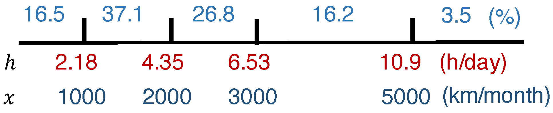Figure 2 shows the charging time per day according to the driving distance distribution for one month. In total, 37.1% of the monthly driving range falls between 1000 and 2000 km, and the charging time ranges from 2.18 to 4.35 h.

2.2. EV Charging Fee

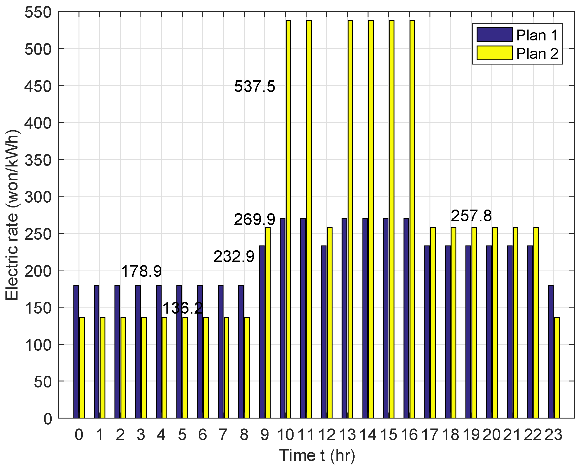
Dynamic rate plans that implement price-based demand response (DR) systems are widely used to reduce the power demand during peak hours or shift it to off-peak hours. A common example of such a plan is the time-of-use (TOU) rate plan, where peak hours of high electricity consumption have higher prices compared to off-peak hours [21]. In this subsection, we analyze the charging fees under a dynamic rate plan using the EV charging model presented in Section 2.

Let s denote the starting time of the charging in hours and $B(s,x)$ denote the charging fee for a driving distance x. Then, $B(s,x)$ can be expressed as

$$\begin{array}{c}\hfill B(s,x):={\int }_s^{s+h}\rho (t \mathrm{m}\mathrm{o}\mathrm{d} 24)r(t \mathrm{m}\mathrm{o}\mathrm{d} 24)dt, \mathrm{f}\mathrm{o}\mathrm{r} 0\le s\le 24.\end{array}$$

(6)

In (6), $r\left(t\right)$, where $0\le t<24$, represents a dynamic rate plan that has varying rates for 24 h a day. If the rate plan $r\left(t\right)$ is a constant of $r_0$ during the charging interval of $s<t<s+h$, then, by using (5), the charging fee in (6) can be rewritten as

$$\begin{array}{c}\hfill B(s,x)=h{r}_0\overline{\rho }=\frac{r_0}{\alpha \eta }x.\end{array}$$

(7)

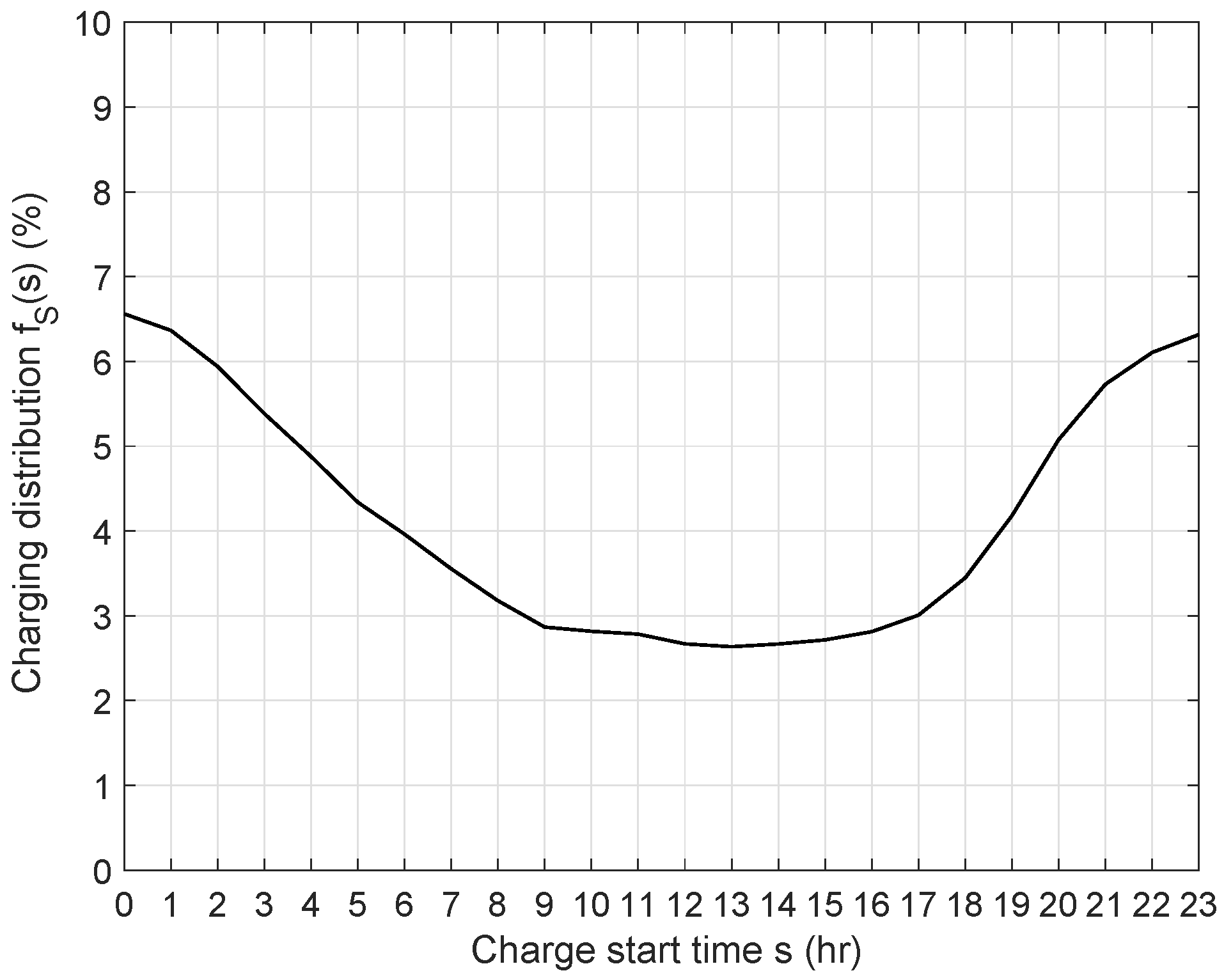
We now derive the mean of the charging fee. First, the starting time of the charging has irregular characteristics, so let us set it as a random variable S instead of a fixed value s. Here, assume that S has a continuous probability density of $f_S$. Furthermore, assume that the driving distance x is set as a random variable X and has a continuous probability density of $f_X$. When the driving distance is given by $X=x$, a mean charging fee is given as the following conditional mean:

$$\begin{array}{c}\hfill E\left\{B(S,x)\right\}=E\left\{B(S,X)|X=x\right\}=\int B(s,x)f_S\left(s\right)ds.\end{array}$$

(8)

For a given driving distance x, we can calculate the daily charging fee using this conditional mean of (8).

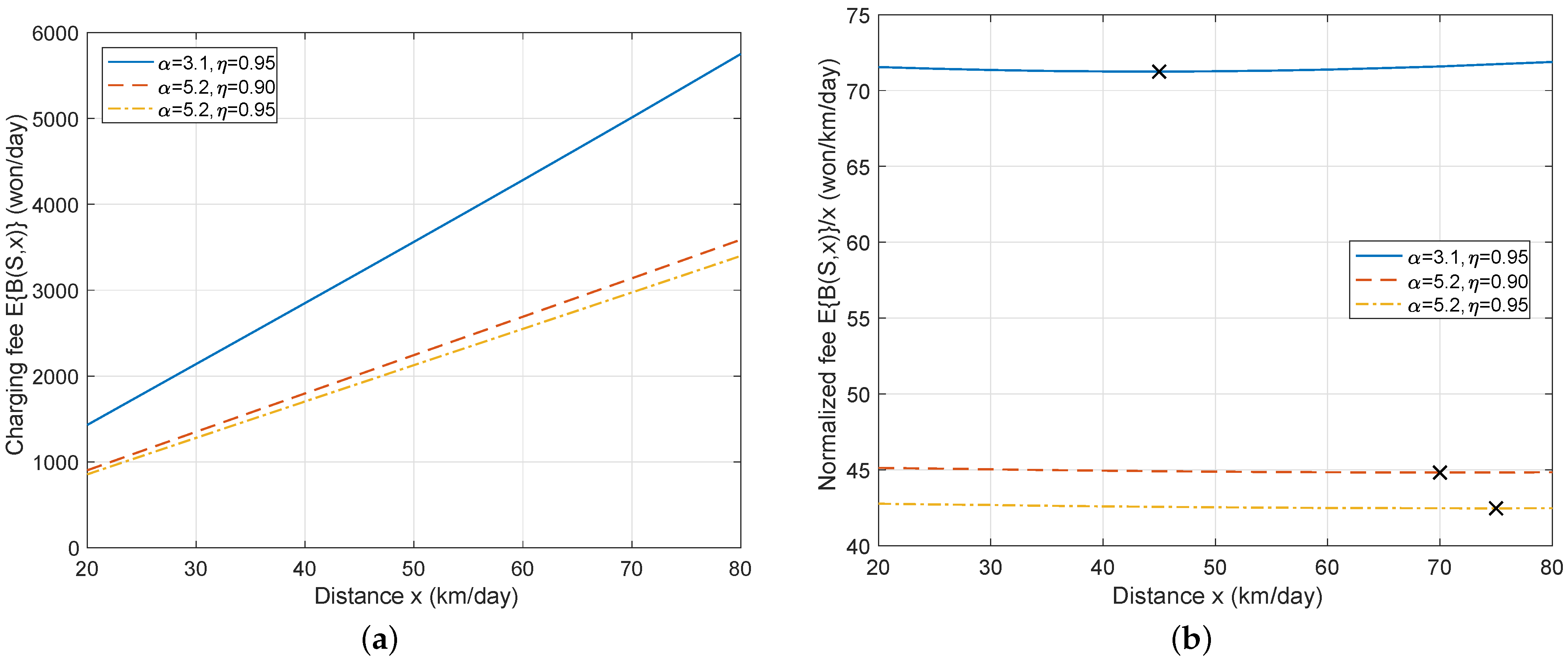
The mean daily charging fee is given as $E\left\{B\right\}=E\left\{B(S,X)\right\}.$ If the rate plan $r\left(t\right)$ is a constant of $r_0$ during a charging interval of t in a similar manner to (7), then the mean charging fee is given as

$$\begin{array}{c}\hfill E\left\{B\right\}=\frac{r_0}{\alpha \eta }E\left\{X\right\}.\end{array}$$

(9)

Assume charging takes place between 23:00 and 09:00. For example, KEPCO provides a fixed rate $r_0=204.6$ KRW/kWh. Note that, as of February 2023, 1000 Korean Won (KRW) is approximately equal to 0.83 US Dollars (USD). For the fuel efficiency of $\alpha =5.2$ km/kWh and the charging efficiency of $\eta =0.95$, the mean charging fee is calculated to be KRW 2524. Here, the mean driving distance is $E\left\{X\right\}=60.94$ km from Figure 2 (KEPRI, 2022). For a membership case of the Korea Electric Vehicle Infrastructure Technology (KEBVIT), the rate is 110 KRW/kWh, and thus, the mean charging fee is KRW 1357.

2.3. Power Load for EV Charging

In this section, the power load required for EV charging is analyzed. Let the instantaneous power load be denoted as $p(t,x)$ at time t. Then, $p(t,x)$ can be written as

$$\begin{array}{c}\hfill p(t,x):={\int }_0^{24}\rho (t \mathrm{m}\mathrm{o}\mathrm{d} 24)\left[u(t-s)-u(t-s-h)\right]f_S\left(s\right)ds\left(\mathrm{k}\mathrm{W}\mathrm{h}\right).\end{array}$$

(10)

From $p(t,x)$ of (10), we can observe the pattern of the required power for charging EVs with respect to t. The peak load, which is obtained from ${max}_{t}p(t,x)$ for a given driving distance x, can be a factor that determines the size of a power installation. For a fixed amount of energy supply, minimizing this peak load is important in reducing the power installation cost. The total amount of supplied energy is $W={\int }_0^{24}p(t,x)dt=h\overline{\rho }$ from (3) and (4), and the mean of the supplied energy is given as

$$\begin{array}{c}\hfill E\left\{{\int }_0^{24}p(t,X)dt\right\}=\frac{E\left\{X\right\}}{\alpha \eta }\left(\mathrm{k}\mathrm{W}\mathrm{h}\right).\end{array}$$

(11)

In addition, the mean power load for each time t is $E\left\{p\right(t,X\left)\right\}$.

3. EV Charging Experiments

In this section, experimental results for the charging time, charging fee, and power load are introduced, with discussions of practical data.

3.1. Charging Time Experiments

In this subsection, we conduct a statistical analysis of the charging time based on the charging model of Figure 1. Based on data from KOSIS, dated 4 August 2022, the daily driving distances of general vehicles are categorized into vehicle types, business use, and non-business use, and summarized in

Table 4. Average daily driving distance (km) for general vehicles in South Korea (KOSIS, South Korea, 4 August 2022).

	Vehicle Types
Business Types	Car	Van	Lorry	Special Car	Average
Non-business use	35.6	33.0	39.6	29.4	36.0
Business use	62.9	139.5	121.4	154.4	85.5
Total	37.2	49.4	49.3	103.3	39.6

. The total average daily driving distance is 39.6 km, which will be used as a representative daily driving distance for EVs. From Table 4, we notice that the driving distance for business use is about 2.4 times that of non-business use. This difference is more pronounced in other vehicle types compared to passenger cars. Due to the significant difference between the driving distances for business and non-business use, it is necessary to set the daily driving distance separately for each case. The daily driving distance is set to 85.5 km for business use and 36.0 km for non-business use.

We now examine the fuel efficiencies of EVs (government-approved compound fuel efficiency, September 2022). The ranking of EV sales in South Korea as of August 2022 is summarized in

Table 5. Domestic electric vehicle sales rankings in South Korea (www.carisyou.com, January–August 2022) and the combined fuel efficiencies (km/kWh) (Government-approved compound fuel efficiency, South Korea, August 2022).

Vehicle	Ioniq 5	EV6	Porter II	Bongo III	Tesla 3
Fuel efficiency	5.2	5.6	3.1	3.1	5.7
Sales (fuel) Ranking	1 (5)	2 (2)	3 (9)	4 (9)	5 (1)
Vehicle	Niro 5	GV60 EV	Tesla Y	GV70 EV	G80 EV
Fuel efficiency	5.3	5.1	5.4	4.6	4.3
Sales (fuel) Ranking	6 (4)	7 (6)	8 (3)	9 (7)	10 (8)

, along with their fuel efficiencies (www.carisyou.com, January to August 2022). Among the vehicles in Table 5, Tesla 3 has the best fuel efficiency of 5.7 km/kWh, and Hyundai Ioniq 5 has a fuel efficiency of 5.2 km/kWh, which will be used in several examples of this paper. On the other hand, trucks such as Porter II and Bongo III have low fuel efficiencies of 3.1 km/kWh. Among these 10 vehicle models, the average combined fuel efficiency of the five vehicle models with higher fuel efficiencies is 5.44 km/kWh, while the average combined fuel efficiency of the remaining five is 4.04 km/kWh. These upper and lower average fuel efficiencies will be used in the subsequent statistical analysis.

Table 6. Combined fuel efficiency (km/kWh) of other vehicles (Government-approved compound fuel efficiency, South Korea, August 2022).

Vehicle	Puegeot e-208	Volt EV	Kona EV	Volvo C40	Ioniq 6
Fuel efficiency	5.4	5.4	5.8	4.1	6.2
Vehicle	VW ID.4	Mini SE	BMW i4	Benz EQS	Audi e-tron
Fuel efficiency	4.7	4.5	4.6	4.0	3.1

provides a summary of the fuel efficiencies for other vehicle models for reference. The Hyundai Ioniq 6 has the highest combined fuel efficiency of 6.2 km/kWh. While most EVs have fuel efficiencies between 4 and 5 km/kWh, Audi’s fuel efficiency is comparatively low at 3 km/kWh.

We now observe the charging times for various vehicle types listed in Table 4 based on the upper and lower mean fuel efficiencies from Table 5.

Table 7. Charging time per day (upper mean fuel efficiency $\alpha =5.44$ km/kWh and $\eta =0.95$).

	Mean Power $\overline{\mathit{\rho }}$ (kW)	Non-Business Use		Business Use		Average
		Car	Van	Car	Van
Distance (km)		35.6	33.0	62.9	139.5	39.6
Charging time (h)	3	2.13	4.06	2.30	9.00	2.55
	2	3.19	6.09	3.44	13.50	3.83

shows the charging times for the upper fuel efficiency of 5.44 km/kWh when charging at a power of $\overline{\rho }=2$ kW and 3 kW. These charging times are calculated using (5). In the case of the total mean of 39.6 km/kWh and $\overline{\rho }=3$ kW, the daily charging time is approximately 2.55 h. For a non-business passenger car, the charging time per day is approximately 2.13 h, while for a business van with a much longer daily driving distance of $x=139.5$ km, the charging time is about 9 h. Table 7 also summarizes the charging times when charging with a reduced power supply of $\overline{\rho }=2$ kW. We can observe that the charging time increases in inverse proportion as the supplied power is reduced by two-thirds.

Table 8. Charging time per day (lower mean fuel efficiency $\alpha =4.04$ km/kWh and $\eta =0.95$).

	Mean Power $\overline{\mathit{\rho }}$ (kW)	Non-Business Use		Business Use		Average
		Car	Van	Car	Van
Distance (km)		35.6	33.0	62.9	139.5	39.6
Charging time (h)	3	2.87	5.46	3.09	11.12	3.44
	2	4.30	8.19	4.64	18.17	5.16

summarizes the daily driving distance for the lower mean fuel efficiency of 4.04 km/kWh. In the case of $\overline{\rho }=3$ kW, the daily charging time is approximately 3.44 h when the total mean driving distance is $x=39.6$ km.

3.2. Charging Fee Experiments

Consider an example of an EV charging fee when a dynamic rate plan is applied, where different times of the day have different rates. The wholesale electricity rate supplied by KEPCO consists of a light-load period (23:00–09:00), a medium-load period (09:00–10:00, 12:00–13:00, and 17:00–23:00), and a maximum-load period (10:00–12:00 and 13:00–17:00), each with different rates. Under this dynamic rate plan, EV charging providers design time-based dynamic rate plans for slow chargers. Examples of such dynamic rate plans are shown in Figure 3 (Plans 1 and 2). Under Plan 1, during the light-load period, the rate is 178.9 KRW/kWh, during the medium-load period, it is 232.9 KRW/kWh, and during the maximum-load period, it is 269.9 KRW/kWh, which is the highest rate.

Figure 4 shows examples of the charging fee $B(s,x)$ when using the rate plans shown in Figure 3. In Figure 4, the x-axis represents the start time s of the charging, and the y-axis represents the charging fee $B(s,x)$. The experiments are conducted using driving distances of $x=20$, 40, and 80 km. Assuming that the fuel efficiency is $\alpha =5.2$ km/kWh, the charging efficiency is $\eta =0.95$, and the mean supplied power is $\overline{\rho }=3$ kW, the charging times for each driving distance are 1.35, 2.70, and 5.40 h from (5). When charging starts at 11:00 p.m., it results in the lowest charging fee for all three distances. For a driving distance of $x=20$ km, the minimum fee can be achieved even if the charging starts at 07:00 a.m. The maximum fee, however, occurs when charging starts at 10:00 a.m. For a relatively long distance of $x=80$ km, the fee is higher than the minimum even if charging starts at 04:00 a.m., and the maximum fee occurs at 10:00 a.m. Thus, in the case of long driving distance per day, it is best to start charging at 11:00 p.m. when the light-load period begins to reduce the charging fee.

Figure 5 shows an example of the distribution $f_S\left(s\right)$ for the charging start time s according to a survey conducted by the Korea Power Exchange (KPX) in June 2021. We notice that the slow chargers are mostly used in the evening and late-night periods after office hours. In Figure 6a, the conditional charging fee $E\left\{B(S,x)\right\}$ of (8) is illustrated using the distribution from Figure 5. In Figure 6, Plan 1 of Figure 3 is used. It is clear that the charging fee increases as the driving distance increases. A low fuel efficiency of $\alpha$ or charging efficiency $\eta$ also increases the charging fee. In Figure 6b, the conditional mean fee for a unit driving distance, $E\left\{B(S,x)\right\}/x$, is shown with respect to the driving distance x. This graph enables us to determine the most economical driving distance for the rates given in Figure 3. It is noted that the slope of the curve is not constant. When $\alpha =5.2$ km/kWh and $\eta =0.95$, the most economical charging fee is obtained at $x=75$ km, as indicated by the lowest normalized charging fee in Figure 6b. However, the savings in cost are not substantial compared to the cases where the driving distance is 20 or 80 km. Note that the shape of the curve representing the normalized charging fee can be different depending on the distribution of the charging start times.

3.3. Power Load Experiments

Figure 7 and Figure 8 show the power load with respect to time for various average driving distances and charging powers from Table 7 and Table 8. Here, the charging efficiency is $\eta =0.95$. For the case of charging power of $\overline{\rho }=3$ kW, the magnitude of the peak load is larger than for the case of $\overline{\rho }=2$ kW. In Figure 7a,b, with the upper mean fuel efficiency of $\alpha =5.44$ km/kWh, as the charging power decreases from 3 to 2 kW, the charging load spreads, resulting in a lower peak load. It is noted that the gradual spread of the charging load comes from the longer charging time required with the lower charging power of 2 kW. From the figures, for the driving distance of 80 km, we observe that the peak load slightly decreases from 0.966 to 0.923 kW. This trend is similarly observed even for the lower mean fuel efficiency case of Figure 8 and for other driving distances.

In Figure 8a, with the lower mean fuel efficiency, the peak load is 1.26 kW at 3:00 a.m. for a driving distance of 80 km. However, in Figure 7a, with the higher mean fuel efficiency, the peak load drops to 0.966 kW at 2:00 a.m. for the same driving distance. Note that this peak load is quite small, and thus, even though 100 EVs of domestic customers charge at night, the peak load is less than 100 kW for the AC slow charges.

4. Discussion

From the peak load experiments, we can observe that the peak load decreases as the supplied power decreases. This property is further demonstrated in Figure 9, which shows the peak load of ${max}_{t}p(t,x)$ with respect to the supplied power $\overline{\rho }$. We observe from Figure 9a that reducing the supplied power slightly decreases the peak load but not by a significant amount when the supplied power is relatively large. For example, at a supplied power of $\overline{\rho }=3$ kW, the peak load is 0.515 kW, and it decreases slightly to 0.513 kW (corresponding to 99.6%), when the supplied power is reduced to 2.5 kW. However, if the supplied power is further reduced to 0.5 kW, the peak load decreases to 0.391 kW (corresponding to 75.9%). Additionally, as shown in Figure 9b, it is observed that as the supplied power decreases, the time when the peak load occurs increases. The conditional charging fee $E\left\{B(S,x)\right\}$ with respect to the supplied power $\overline{\rho }$ is also shown in Figure 10a for a driving distance of $x=39.6$ km. As the supplied power decreases from 3 kW, the charging fee also decreases and reaches a minimum of KRW 1682 at $\overline{\rho }=1.61\mathrm{kW}$. Therefore, at this supplied power, we can reduce both peak load and charging fee. However, further decreasing the supplied power can increase the charging fee, as illustrated in Figure 10a. Thus, the supplied power of $\overline{\rho }=1.61\mathrm{kW}$ can be a good choice for minimizing the charging fee. In Figure 10b, the optimally supplied power is shown with respect to the driving distance. We observe that the optimal supplied power increases as the driving distance increases.

Figure 11 shows the peak load curves with respect to fuel and charging efficiencies. As shown in these figures, it is clear that vehicles with high fuel or charging efficiency can reduce the peak load. For the example of Figure 11a, the peak load is 0.658 kW at the fuel efficiency of $\alpha =4.04$. However, if the fuel efficiency is improved to $\alpha =5.44$, then the peak load decreases to 0.493 kW, which corresponds to a significant increase of 25.1%. For the charging efficiency case in Figure 11b, increasing the efficiency from 0.95 to 0.98 improves the peak load from 0.515 to 0.500 kW, which corresponds to only a 2.9% reduction. Therefore, to reduce the peak load, developing vehicles with high fuel efficiencies is more important rather than focusing on the charging efficiency.

In Figure 12, the charging fee and load power curves of Class 3 kW are compared with those of Class 7–11 kW. For both driving distances of 40 and 80 km, Class 3 kW has slightly lower charging fees than Class 7–11 kW. In the peak load case, Class 3 kW also shows slightly better performance than Class 7–11 kW. Therefore, in terms of the charging fee and peak load, we notice that Class 3 kW is slightly better than Class 7–11 kW. It should be noted that the implementation cost of Class 3 kW is much lower than that of Class 7–11 kW. Hence, Class 3 kW can be a good choice for EV charging with low implementation cost.

5. Conclusions

In this paper, under a daily charging scenario, a simple EV charging model was developed for AC slow chargers, and the performance of a charger for Class 3 kW was analyzed. In this charging scenario, we can use cheaper batteries with lower capacities and energy densities [22,23]. Using the slow charger model, we calculated the required charging times for different charging efficiencies and various vehicle types, as well as the charging fees based on dynamic charging rate plans. Both the charging time and fee are linearly proportional to the driving distance, and vehicles with low fuel or charging efficiencies result in higher charging fees. We also observed the peak load for charging under various parameters, noting that decreasing the supplied power decreases the peak load. Slightly decreasing the supplied power can lower the charging fee, but further decreasing it can increase the fee. An optimal supplied mean power exists for a given driving distance, and this increases as the distance increases. Increasing the fuel efficiency or charging efficiency can reduce the peak load. Additionally, we compared the slow charger of Class 3 kW with Class 7–11 kW and found that Class 3 kW performs slightly better with a lower implementation cost than Class 7–11 kW.

References

1. Nanaki, E.A.; Koroneos, C.J. Climate change mitigation and deployment of electric vehicles in urban areas. Renew. Energy 2016, 99, 1153–1160. [Google Scholar] [CrossRef]
2. OECD/IEA. Energy Technology Perspectives 2010; OECD/IEA: Paris, France, 2010. [Google Scholar]
3. Bloomberg. Electric Vehicle Outlook 2017. Bloomberg New Energy Finance; Bloomberg: New York, NY, USA, 2017. [Google Scholar]
4. Bloomberg. Electric Vehicle Outlook 2020. Bloomberg New Energy Finance; Bloomberg: New York, NY, USA, 2022. [Google Scholar]
5. Ucer, E.; Koyuncu, I.; Kisacikoglu, M.C.; Yavuz, M.; Meintz, A.; Rames, C. Modeling and analysis of a fast charging station and evaluation of service quality for electric vehicles. IEEE Trans. Transp. Electrif. 2019, 5, 215–225. [Google Scholar] [CrossRef]
6. SAE International. Charging Configurations and Ratings Terminology-SAE Hybrid Committee; SAE International: Warrendale, PA, USA, 2022. [Google Scholar]
7. Tavakoli, A.; Saha, S.; Arif, M.; Haque, M.; Mendis, N.; Oo, A.M.T. Impacts of grid integration of solar PV and electric vehicle on grid stability, power quality and energy economics: A review. IET Energy Syst. Integr. 2020, 2, 243–260. [Google Scholar] [CrossRef]
8. Dharmakeerthi, C.; Mithulananthan, N.; Saha, T. Impact of electric vehicle fast charging on power system voltage stability. Int. J. Electr. Power Energy Syst. 2014, 57, 241–249. [Google Scholar] [CrossRef]
9. Wang, Z.; Paranjape, R. An evaluation of electric vehicle penetration under demand response in a multi-agent based simulation. In Proceedings of the 2014 IEEE Electrical Power and Energy Conference, Calgary, AB, Canada, 12–14 November 2014; pp. 220–225. [Google Scholar]
10. Birk Jones, C.; Vining, W.; Lave, M.; Haines, T.; Neuman, C.; Bennett, J.; Scoffield, D.R. Impact of electric vehicle customer response to time-of-use rates on distribution power grids. Energy Rep. 2022, 8, 8225–8235. [Google Scholar] [CrossRef]
11. Suski, A.; Remy, T.; Chattopadhyay, D.; Song, C.S.; Jaques, I.; Keskes, T.; Li, Y. Analyzing electric vehicle load impact on power systems: Modeling analysis and a case study for maldives. IEEE Access 2021, 9, 125640–125657. [Google Scholar] [CrossRef]
12. Kühnbach, M.; Stute, J.; Klingler, A.L. Impacts of avalanche effects of price-optimized electric vehicle charging—Does demand response make it worse? Energy Strategy Rev. 2021, 34, 100608. [Google Scholar] [CrossRef]
13. Singh, S.; Pamshetti, V.B.; Singh, S.P. Time horizon-based model predictive Volt/VAR optimization for smart grid enabled CVR in the presence of electric vehicle charging loads. IEEE Trans. Ind. Appl. 2019, 55, 5502–5513. [Google Scholar] [CrossRef]
14. Dulău, L.I.; Bică, D. Effects of electric vehicles on power networks. Procedia Manuf. 2020, 46, 370–377. [Google Scholar] [CrossRef]
15. Yi, F.; Zeng, P.; Yu, S.; Gu, C.; Li, J.; Yuan, C.; Li, F. Impacts of classified electric vehicle charging derived from driving patterns to the LV distribution network. In Proceedings of the 2014 IEEE PES General Meeting|Conference & Exposition, National Harbor, MD, USA, 27–31 July 2014; pp. 1–5. [Google Scholar]
16. Kuspan, B.; Bagheri, M.; Abedinia, O.; Naderi, M.S.; Jamshidpour, E. The influence of electric vehicle penetration on distribution transformer aging rate and performance. In Proceedings of the 2018 7th International Conference on Renewable Energy Research and Applications (ICRERA), Paris, France, 14–17 October 2018; pp. 313–318. [Google Scholar]
17. Pradhan, P.; Ahmad, I.; Habibi, D.; Kothapalli, G.; Masoum, M.A.S. Reducing the impacts of electric vehicle charging on power distribution transformers. IEEE Access 2020, 8, 210183–210193. [Google Scholar] [CrossRef]
18. Akil, M.; Dokur, E.; Bayindir, R. Impact of electric vehicle charging profiles in data-driven framework on distribution network. In Proceedings of the 2021 9th International Conference on Smart Grid (icSmartGrid), Setubal, Portugal, 9 June–1 July 2021; pp. 220–225. [Google Scholar]
19. Locorotondo, E.; Corti, F.; Pugi, L.; Berzi, L.; Reatti, A.; Lutzemberger, G. Design of a wireless charging system for online battery spectroscopy. Energies 2021, 14, 218. [Google Scholar] [CrossRef]
20. Cittanti, D.; Ferraris, A.; Airale, A.; Fiorot, S.; Scavuzzo, S.; Carello, M. Modeling Li-ion batteries for automotive application: A trade-off between accuracy and complexity. In Proceedings of the 2017 International Conference of Electrical and Electronic Technologies for Automotive, Torino, Italy, 15–16 June 2017; pp. 1–8. [Google Scholar]
21. Chung, Y.M.; Kang, S.; Jung, J.; Chung, B.J.; Kim, D.S. Residential electricity rate plans and their selections based on statistical learning. IEEE Access 2022, 10, 74012–74022. [Google Scholar] [CrossRef]
22. Locorotondo, E.; Cultrera, V.; Pugi, L.; Berzi, L.; Pasquali, M.; Andrenacci, N.; Lutzemberger, G.; Pierini, M. Impedance spectroscopy characterization of lithium batteries with different ages in second life application. In Proceedings of the 2020 IEEE International Conference on Environment and Electrical Engineering and 2020 IEEE Industrial and Commercial Power Systems Europe (EEEIC/I&CPS Europe), Madrid, Spain, 9–12 June 2020; pp. 1–6. [Google Scholar]
23. Alipour, M.; Ziebert, C.; Conte, F.V.; Kizilel, R. A review on temperature-dependent electrochemical properties, aging, and performance of lithium-ion cells. Batteries 2020, 6, 35. [Google Scholar] [CrossRef]
Figure 1. EV charging model for the AC slow charger. The AC power is supplied from a regular AC 220 V outlet a the maximum current of 16 A to the OBC, which converts the AC power to DC power and charges the battery.
Energies 16 02735 g001
Figure 2. Distribution example of the driving distance x (KEPRI, 2022). Average driving distance per month is 1889 km ( x = 60.9 km).
Energies 16 02735 g002
Figure 3. Examples of the slow-rate plan r ( t ) (KRW 1000 is USD 0.83).
Energies 16 02735 g003
Figure 4. Charging fee B ( s , x ) of (6) when charging with the rate plans of Figure 3 ( α = 5.2 km/kWh, η = 0.95 , ρ ¯ = 3 kW, and KRW 1000 is USD 0.83).
Energies 16 02735 g004
Figure 5. Example of the charging start time distribution f S : slow charger usage over the time interval (KPX, June 2021).
Energies 16 02735 g005
Figure 6. Charging fee example for Plan 1 of Figure 3 and the distribution f S of Figure 5, when the supplied power is ρ ¯ = 3 kW (KRW 1000 is USD 0.83). (a) Conditional mean charging fee E B ( S , x ) of (8). (b) Normalized conditional charging fee E B ( S , x ) / x .
Energies 16 02735 g006
Figure 7. Power load curves p ( t , x ) for each time interval of Table 7 with the upper mean fuel efficiency of α = 5.44 km/kWh. The charging start time distribution of Figure 5 is used, and the charging efficiency is η = 0.95 . (a) The charging power is ρ ¯ = 3 kW. The maximum power of x = 80 km is 0.966 kW at 2:00 a.m. (b) The charging power is ρ ¯ = 2 kW. The maximum power of x = 80 km is 0.923 kW at 3:00 a.m.
Energies 16 02735 g007
Figure 8. Power load curves p ( t , x ) for each time interval of Table 8 with the lower mean fuel efficiency of α = 4.04 km/kWh. The charging start time distribution of Figure 5 is used and the charging efficiency is η = 0.95 . (a) The charging power is ρ ¯ = 3 kW. The maximum power of x = 80 km is 1.26 kW at 3:00 a.m. (b) The charging power is ρ ¯ = 2 kW. The maximum power of x = 80 km is 1.17 kW at 5:00 a.m.
Energies 16 02735 g008
Figure 9. Peak load and time with respect to the charging mean power ( α = 5.2 km/kWh, η = 0.95 , and x = 39.6 km). (a) Peak load max t p ( t , x ) with respect to ρ ¯ . (b) Peak load time arg max t p ( t , x ) with respect to ρ ¯ .
Energies 16 02735 g009
Figure 10. Charging fee E B ( S , x ) with respect to the supplied power ρ ¯ for the slow-rate plans and the charging start time distribution f S of Figure 5 ( α = 5.2 km/kWh, η = 0.95 , and KRW 1000 is USD 0.83). (a) Charging fee curve for the driving distance of x = 39.6 km. The minimum charging fee is KRW 1682 at ρ ¯ = 1.61 kW. (b) Optimal supplied mean power with respect to the driving distance.
Energies 16 02735 g010
Figure 11. Peak loads from max t p ( t , x ) ( x = 39.6 km and ρ ¯ = 3 kW). (a) Peak load with respect to the fuel efficiency α for η = 0.95 . (b) Peak load with respect to the charging efficiency η for α = 5.2 km/kWh.
Energies 16 02735 g011
Figure 12. Comparison of the slow chargers of Class 3 kW and Class 7–11 kW for Plan 1 of Figure 3 ( x = 39.6 km, α = 5.44 km/kWh, η = 0.95 , and KRW 1000 is USD 0.83). (a) Charging fee B ( s , x ) and E { B ( S , x ) } . (b) Load power p ( t , x ) and the peak load max t p ( t , x ) .
Energies 16 02735 g012