Integrated Assessment of Economic Supply and Environmental Effects of Biomass Co-Firing in Coal Power Plants: A Case Study of Jiangsu, China

Abstract

The technical supply potential of biomass and the associated greenhouse gas (GHG) emissions are widely studied in the literature. However, relatively few studies have examined the role of biomass co-firing for future electricity in China by integratedly considering the economic supply potential and GHG effects. To fill this gap, we choose the Jiangsu Province in China as a case study and build up a partial equilibrium model with multiple agricultural commodities. Using this model combined with a life cycle assessment, we jointly determine the economic potential of the biomass supply for a biomass co-firing purpose and social benefits, including the agricultural producers’ surplus and GHG mitigation potential. The simulation incorporates the county-level biomass market of various crop residues as well as endogenous crop prices and transportation costs. We find that 0.7–12.5 M MT of residue-based biomass are economically viable for co-firing in coal-based power plants (up to 20%) at biomass prices between USD 50 and USD 100/MT. The net GHG savings achieved at these biomass prices are from 3.2 to 59 M MTCO₂e. Our findings indicate that biomass co-firing with coal in power plants would be a feasible low-carbon energy transition pathway if the biomass price is above USD 50/MT. In addition to biomass prices, other factors such as crop yields, production costs of residues, and transportation costs are found to be impactful on the economic viability of biomass and GHG savings. Our results can inform policy to develop localized carbon reduction strategies in provinces with abundant biomass resources and a high share of coal-fired electricity.

1. Introduction

Climate change has become a global concern in recent decades. A number of countries worldwide have begun to undertake efforts to tackle climate change. In 2020, China pledged to achieve its carbon neutrality goal by 2060. A significant step forward was made at the 26th annual United Nations Climate Change Conference (COP26), when China, along with 196 other parties, agreed on curbing fossil fuel usage and phasing down unabated coal power [1]. Following the Chinese government’s pledge, the county’s energy system has been undergoing a transformation by gradually shifting away from fossil fuels toward renewable energy sources such as wind, solar, water, and biomass [2]. While being responsible for nearly 50% of global renewable capacity additions in 2020, China faces great challenges in achieving a rapid coal phaseout in the near term. The overwhelming amount of large and new coal infrastructure has made the government cautious about setting a coal power phaseout schedule [3]. In addition, the geographical mismatch between the supply of wind and solar power and the demand for energy results in the large curtailment of renewable energy [4]. Conflict between the economic and environmental objectives limited the Chinese government’s ability to make more pledges at the recent 27th annual conference (COP27). These challenges further raise skepticism about whether China can decarbonize its power system within the expected timeline. In recent years, bioenergy, particularly biomass–coal co-firing, has attracted increasing interests mainly for three reasons. First, it is cost-effective for decarbonizing coal fleets without incurring the high costs of retrofitting. Second, biomass–coal co-firing for electricity generation offers co-benefits such as enhancing energy security, providing extra revenue for farmers, and reducing air pollution from crop residue burning. Third, when combined with carbon capture and storage, it can serve as a key negative emission solution for achieving climate goals [5]. Although biopower has not been deployed at a large scale, it has been proposed as an attractive solution for decarbonizing the energy system in regions with the considerable potential to have a biomass supply and a high share of coal-fired electricity.

China is the world’s largest emitter of greenhouse gases (GHG) because of the large share of the heavy industry sector and emissions-intensive energy mix. In 2020, coal-fired power and heat generation alone were responsible for nearly 50% of the country’s energy-related CO₂ emissions [6]. Jiangsu Province, located on the eastern coast of China, ranks as the second-largest province by economy and energy consumption. It is also the third-largest province for coal-fired power generation in China. Approximately 439 billion kWh of electricity were produced in coal-based power plants in 2020, accounting for 87% of the total electricity generation in the province [7]. While Jiangsu is among the top provinces for electricity generation, it faces an electricity supply shortage due to a lack of coal reserves; hence, it has actively promoted the development of renewable energy resources to supersede coal consumption [8].

Recently, Jiangsu was among the leading Chinese provinces for bioenergy generation, with a total installation capacity exceeding 1000 megawatts (MW) [9]. However, biomass co-firing in coal power plants has not received sufficient policy support, and the development is much slower than expected. This is primarily attributed to concerns regarding the adequacy of biomass resources and the environmental impacts associated with large-scale biomass production [10]. Therefore, understanding the optimal location and quantity of biomass that can be supplied to specific power plants is crucial for the economic and sustainable development of the biopower industry. Along with economic factors, there are environmental issues that require rigorous estimates. For instance, heightened biomass demand is likely to impact the crop mix and land-use change, which in turn affects the aboveground emissions and soil carbon emissions [11]. In addition, energy uses during the process of biomass harvesting and transportation may offset part of the GHG benefits from coal replacement. Therefore, a systematic evaluation of the economic and environmental consequences of biomass-based power generation can inform renewable energy policy decisions and promote feasible low-carbon energy transition pathways in Jiangsu.

Previous studies on bioenergy evaluation focused on the potential supply of biomass and costs along the supply chain, either regionally [12,13,14] or nationally in China [15,16,17]. By applying remote-sensing data, Qiu et al. [16] estimated that about 147–334 million metric tons (M MT) of crop residues could be used to replace coal in 2010. Similarly, Qin et al. [18] estimated that about 280 M MT of crop-residue-based biomass and more than 150 M MT of energy crops are available for bioenergy each year. Kang et al. [19] discovered that the collectable potential of China’s total biomass resources (including crop residues, forest residues, energy crops, animal manure, municipal solid waste, etc.) reached 32.69 EJ, corresponding to 27.6% of the total energy consumption. They also found that the Henan, Shandong, Jiangsu, and Guangxi provinces are the four most important provinces for the development of the bioenergy industry. Recently, Xing et al. [20] estimated that 3.04 GT/year of cellulosic biomass could be theoretically harvested in China, with 64% being energy crops and 26% being agricultural residues. In general, existing estimates suggest that China has a notable potential for its cellulosic biomass supply. However, these studies only considered the technical potential of residues production and overlooked economic factors (e.g., land rent, production costs, and biomass prices). Among the limited studies integrating agricultural commodity markets, Chen [21] assessed the economic potential of the residue biomass supply on a national scale and found that China could potentially produce about 174.4 to 248.6 M MT of crop residues at a biomass price of USD 150/MT, depending on the yields and costs of crop residues. However, they did not explicitly model the supply chain networks of the crop residues for co-firing with coal at power plants nor did they use any domestic crop residue production costs due to a lack of relevant data.

Many cost and procurement studies examined the effects of different cost components on the profitability of the bioenergy industry. For instance, Zhang et al. [8] identified biomass prices and transportation costs as the primary factors for the deficit of straw-fired power-generation plants in Jiangsu Province. A recent study by Fang et al. [22] examined the wheat straw logistics systems and found that the harvest rate and transportation capacity were crucial to the sustainable development of the bioenergy industry. Li et al. [23] conducted a unit-level cost–benefit analysis of biomass co-firing retrofitting at the national level and pointed out that the installed capacity, operating year, and transportation distance were important influencing factors on the heterogeneity of the economic cost. Even though these analyses were mostly carried out at the facility level, their findings suggest that it is important to incorporate cost and logistic information in the biomass supply potential evaluation. Moreover, a purely technical analysis without considering farmers’ willingness to collect and other economic factors may overestimate the actual supply potential [21].

The environmental implications of bioenergy systems vary with different studies and have become the subject of debate. Many previous studies estimated the GHG outcomes of producing bioenergy with various cellulosic biomass and concluded that substituting fossil fuels with bioenergy could significantly reduce GHG emissions [18,24,25,26]. However, some other studies showed opposite opinions and suggested that support policy should shift away from bioenergy toward natural-based solutions such as grassland restoration and reforestation/afforestation [27,28]. Particularly, the harvest of crop residues raised concerns about GHG emissions because high residue removal rates may affect soil carbon stocks [29]. The multifaceted nature of biopower production calls for a sophisticated modeling approach when assessing its supply and mitigation potential [30].

The techno-economic model has been widely adopted to evaluate the feasibility of bioenergy production with various biomass feedstocks [31,32] and conversion technologies [33,34]. Such analyses typically investigated the performance of a bioenergy process by incorporating the economic and technical parameters in a bottom-up model. An increasing number of studies further extended the traditional techno-economic analysis by including the environmental dimension to address both the economic and sustainability issues with the bioenergy system [35]. The system boundaries of these studies were often limited to the bioenergy process, hence neglecting the supply chain and crop/biomass market impacts [36]. Integrated assessment models (IAMs), such as IMAGE and GCAM, are often used to investigate least-cost energy transition pathways, including bioenergy development [30,37,38]. The highly aggregated structure of energy and land systems makes IAMs not an ideal tool for studying the biomass supply potential at the subnational level. Computable general equilibrium (CGE) models with comprehensive coverage of multiple sectors and economic activities are well-suited to assess the effects of certain bioenergy expansion policies or shocks across different sectors; however, they lack the flexibility of adding details to an analysis of the related sectors. Partial equilibrium (PE) models, which have the advantages of representing spatial heterogeneity in biomass production, are adopted to estimate the biomass supply potential. PE models such as BEPAM [39] and the one developed by Chen [21] endogenously determined the optimal land use and feedstock mix by maximizing the sum of consumers and producers’ surplus for multiple sectors (i.e., agriculture, forest, electricity, etc.). However, these PE models assumed the average costs for sourcing feedstocks to representative biorefinery or biopower locations, which could potentially misrepresent the economic supply potential.

Despite the rich literature on the biomass supply potential in China, there are still knowledge gaps concerning the economically available biomass for co-firing with coal and associated GHG mitigation potentials at the subnational level. Therefore, the aims of this paper are, firstly, to examine the economically viable supply of crop residues and the spatial distribution of residues at various biomass prices and, secondly, to estimate the GHG mitigation potential of biomass co-firing with coal for electricity generation. We choose to focus on Jiangsu Province, as it is a typical province facing a strong conflict between economic growth and environmental objectives [8]. In addition, it has a good opportunity for the development of the coal–biomass co-firing industry, given its current leading role in bioenergy production.

In this study, we developed a static, partial equilibrium, nonlinear mathematical programming model of the agricultural sector. This model endogenously determines the land allocation, crop production, and prices in markets for the food crops in Jiangsu. We also incorporated supply chain information, such as the choice of co-firing units, feedstocks, and biomass production locations into the model. A GHG life cycle assessment was further linked to the model to account for the GHG emissions related to farming activities, soil carbon sequestration, biomass transportation, and the conversion process. The novel integrated modeling framework considers the agricultural and biomass market effects, by including multiple agricultural commodities and different types of crop residues, and accounts for spatial heterogeneity in the biomass supply and coal plant sites. This paper contributes to the existing literature in two aspects. First, unlike previous studies that focused on the technical potential of the biomass supply, we examine biomass availability under various market-driven conditions. Second, we explore the energy–environment nexus by estimating the optimal harvesting of biomass at the county level and the implications for the GHG emissions and social welfare associated with biomass co-firing electricity generation. These effects, to our knowledge, were rarely systematically examined in the literature. The outcomes of this study are meaningful to local decision makers to identify the appropriate low-carbon transition pathway for the power sector. Furthermore, our findings have broad implications for other regions sharing similar topography and biomass potentials and heavily relying on coal to meet their electricity demands.

2. Simulation Model

The mathematical programming model draws from key agricultural and energy sector data sources to develop a detailed representation of the supply points within all counties and the demand points (existing coal power plants) throughout Jiangsu Province. The model covers seven major crops: corn, wheat, rice, soybean, cotton, peanut, and rapeseed. The planted area for these crops was 5.48 million hectares (M ha) in the base year 2020, accounting for 96% of the total cropland in the province. We developed the model from a social planner’s perspective, which maximizes the sum of the producers and consumers’ surplus within the agricultural market subject to various material balance and technological and land availability constraints. It endogenously determines the quantities of row crops and their market prices, ensuring that market demand and supply are in equilibrium. The model also exogenously sets biomass prices to trigger economic incentives for the reallocation of land among various row crops until a new equilibrium is achieved in the market. The overall structure of the model is presented in Figure 1.

The mathematical representation of the main functions in the model is described in the remainder of this section. For clarity, in the following algebraic illustration, the exogenous parameters/data are denoted using lower-case symbols, while the endogenously determined variables are represented by upper-case symbols. Equation (1) is an objective function that represents the sum of welfare in the agricultural sector. The consumers and producers’ surpluses are obtained from the production and consumption of various agricultural commodities.

$$\mathrm{M}\mathrm{a}\mathrm{x}:p\sum _{i,r}{BMASS}_{i,r}+\sum _i{\int }_0^{Q_i}{P}_i\left(q\right)d\left(q\right)-\sum _{i,r}{rc}_{i,r}{L}_{i,r}-\sum _{i,r}{rs}_{i,r}{BMASS}_{i,r}$$

(1)

The first term of the objective function represents the revenues from collecting crop residues at a market biomass price, $p$. The biomass price is exogenously given to induce the collection of crop residues. The second term denotes the sum of the areas under the demand functions from which consumers derive surplus from the consumption of various crop commodities. $P_i\left(q\right)$ represents the inverse domestic demand function for crop $i$, where $q$ is the integration variable. $Q_i$ denotes the endogenous domestic demand for crop $i$. The third term includes the costs of crop production. The planted acreage allocated to crop $i$ in county r is denoted by $L_{i,r}$. ${rc}_{i,r}$ denotes the production cost of crop $i$ per unit of land in county r. A Leontief production function is assumed for crop production. The fourth term represents the costs of collecting, processing, storing, and transporting residues, where ${rs}_{i,r}$ and ${BMASS}_{i,r}$ denote the residue cost per unit of collected residue and the collected crop residues for crop $i$ and county r, respectively. The objective function is quadratic, given the linear specifications of the domestic demand functions. Note that the crop prices solved in the model represent producer prices at the farm gate, since we did not consider the transportation of crops to consumers.

$$Q_i\le \sum _r{y}_{i,r}{L}_{i,r}\hspace{1em}\forall i$$

(2)

Equation (2) is the material balance constraint indicating that the sum of domestic demands is restricted to the total production of that crop. Given that the self-sufficiency ratio of the main crop commodities in Jiangsu is around 100% and that most of them are consumed domestically, we did not, thus, consider the import and export of the crops. $y_{i,r}$ denotes the yield of crop $i$ per unit of land in county $r$.

$${BMASS}_{i,r}\le {yr}_{i,r}{LR}_{i,r}\hspace{1em}\forall i,r$$

(3)

Equation (3) relates the total production of crop residues to the supply at the county level. ${yr}_{i,r}$ denotes the yield per unit of crop residue under crop $i$ in county r. ${LR}_{i,r}$ represents the amount of land under which crop residues are collected under crop $i$ in county r.

$${\sum }_i^{ }{L}_{i,r}\le {land}_r\hspace{1em}\hspace{1em}\forall r$$

(4)

$${LR}_{i,r}\le L_{i,r}\hspace{1em}\hspace{1em}\forall i,r$$

(5)

The land available for crop production is subject to Constraint (4), stating that the sum of land allocated to different types of crops in a county cannot exceed the total land availability in that county (denoted by ${land}_r$). Constraint (5) requires that the land from crop residues cannot exceed the amount of land allocated to the crop that produces the corresponding type of crop residue. Following Chen [21], we also imposed historical crop mix constraints to avoid extreme specialization in regional land use and crop production, as shown in Equations (6) and (7).

$${\theta }_{i,r}{L}_{i,r}={\sum }_{hy}^{ }{h}_{i,r,hy}{W}_{i,r,hy}\hspace{1em}\hspace{1em}\forall i,r$$

(6)

$${\sum }_{hy}^{ }{W}_{i,r,hy}\le 1\hspace{1em}\hspace{1em}\forall i,r$$

(7)

We restricted farmers’ planting decisions to a convex combination of historically observed acreage patterns, ($h_{i,r,hy}$), where subscript $hy$ stands for the periods from 2000 to 2020. ${\theta }_{i,r}$ represents the share of row crop $i$ in county r. $W_{i,r,hy}$ represents the weight assigned to historical crop mixes. The sum of the endogenous weights assigned to individual mixes must be less than or equal to 1, as shown in Equation (7).

$${\sum }_{i,r}^{ }{RES}_{i,r,k}\le \left(\frac{\gamma }{1-\gamma \times \alpha }\right)\times ({hi}_k\times {oh}_k\times c)/{cv}_{coal}\hspace{1em}\forall k$$

(8)

$$\alpha =1-\frac{{CV}_{bio}}{{CV}_{coal}}$$

(9)

$${hi}_k={np}_k\times f_k/{\rho }_k\hspace{1em}\hspace{1em}\forall k$$

(10)

$${\sum }_k^{ }{RES}_{i,r,k}={BMASS}_{i,r}\hspace{1em}\hspace{1em}\forall i,r$$

(11)

Equation (8) represents a capacity constraint that limits the total residue consumption at a facility level as no greater than the co-firing capacity of the coal boilers. The right-hand side of Equation (8) calculates the total amount of biomass required to displace coal at a certain co-firing level, adopted from the formula in [40]. Parameter $\alpha$ depends on the calorific value of the coal and biomass, as given by Equation (9). ${cv}_{coal}$ is the calorific value of coal, which is 21.81 MMBTU/MT (23.06 MJ/kg) [41]; ${cv}_{bio}$ is the calorific value of biomass, which is 17.72 MJ/kg dry matter [42]. The heat input (${hi}_k$) for each facility is a function of the plant’s nameplate capacity in MW (${np}_k$), capacity factor ($f_k$), and plant efficiency rate (${\rho }_k$). ${oh}_k$ is the total number of operating hours (in hr/year). $c$ is the conversion factor from MW to BTU/hr. For simplicity, we assumed that there would be no equipment efficiency loss due to co-firing. $\gamma$ is an arbitrary, exogenous parameter used to restrict the co-firing capacity. We developed two co-firing scenarios for which $\gamma$ can be 10% and 20% on a heat-input basis, by considering that the common co-firing ratio using current technology is between 10% and 20% [43]. Biomass-dedicated power plants that use 100% biomass feedstocks are not the focus in our study given their very limited capacity in the area. Our model allows for the endogenous determination of which facilities can utilize the crop residues supplied from which counties. ${RES}_{i,r,k}$ represents the amount of co-firing crop residues consumed by facility $k$ sourced from county $r$ and of type $i$. Equation (11) requires the sum of the residues consumed by facilities sourced from county $r$ and type $i$ to be equal to the collected biomass in that county.

The modeling methodology applied here advances the existing approaches in two aspects. First, in contrast to the previous spatially explicit optimization models, which are usually based on producers’ cost-minimization objectives [20,44], we estimated the supply curves of various residues from a social planner’s perspective, by optimizing the total welfare of the agricultural producers and consumers. This approach better serves our purposes to identify the economic potential of the biomass supply and derive bioenergy policy implications. Additionally, unlike other bioenergy assessment models that commonly operate at a state/province or coarser scale [19,38], we conduct modeling at a finer county level to obtain a more realistic representation of the biomass production and road network.

3. GHG Savings with Biopower

We calculated the total GHG emission from 100% coal-based electricity using Equation (12):

$${GHG}_{coal}=Q_{coal}\times {EF}_{coal}$$

(12)

where $Q_{coal}$ is the total amount of coal-based electricity, in kWh. $EFcoal$ is the emission factor of coal-based electricity, which is 1230 g CO₂e/kWh [45].

The total emission from biopower was calculated using Equation (13).

$${GHG}_{bio}={GHG}_{harv}+{GHG}_{proc}+{GHG}_{tran}{+GHG}_{burn}$$

(13)

where ${GHG}_{harv}$ is the farm gate GHG emission due to the harvesting operation of crop residues, including planting, cultivating, and harvesting crops and crop residues; ${GHG}_{proc}$ is the GHG emission with the preprocessing of biomass including crushing, baling, carrying, storing, etc. Two emerging technologies, including pelletization and torrefaction that were mentioned in some studies, are not considered here because they are too expensive and GHG-intensive [41,46]. ${GHG}_{tran}$ is the GHG emission from the biomass transportation from the collection field to the power plants; ${GHG}_{burn}$ represents the GHG emission from the burning of biomass for electricity generation. This emission corresponds to the non-biogenic carbon emission from the electricity production process. In addition, we explicitly took account of the change in CH₄ emissions with rice cultivation due to increased residue demand. However, the soil carbon change with land conversion cross different crops was excluded from the analysis due to the lack of available data. Emission factors involved in each stage are presented in the Supplementary Information Table S1.

We estimated the net GHG savings from replacing coal with biomass using Equation (14):

$${GHG}_{saving}={GHG}_{coal}-{GHG}_{coal}^{\prime }-{GHG}_{bio}{+GHG}_{straw}$$

(14)

where ${GHG}_{saving}$ is the net GHG saving in metric tons of CO₂ equivalent. ${GHG}_{coal}$ is the GHG emission with coal-based electricity at the zero-biomass price; ${GHG}_{coal}^{\prime }$ is the GHG emission with coal-based electricity at the non-zero-biomass price; ${GHG}_{coal}-{GHG}_{coal}^{\prime }$ represents the emissions avoided by replacing coal in the power plant. We also considered the avoided emissions from residue open burning, which is represented by ${GHG}_{straw}$. If there is no commercial value for crop residues, farmers would be more likely to burn them in their fields [47].

We calculated the GHG emissions from the crop residues’ open burning by using Equation (15), following [48]. Crop residue open burning can emit CO₂, CH₄, and N₂O; however, only CH₄ and N₂O emissions are relevant due to the carbon neutrality assumption for biomass.

$${GHG}_{straw}={\sum }_{i,r}^{ }{BMASS}_{i,r}\times f_{burn}\times {EF}_{crop}\times GWP$$

(15)

where $f_{burn}$ is the burning efficiency, 0.9 [48]; ${EF}_{crop}$ is the emission factor, which is 3.23 g CH₄/kg for CH₄ and 0.008 g N₂O/kg for N₂O; and GWP is the global warming potential on a 100 year horizon, which is 28 for CH₄ and 265 for N₂O [49].

4. Data

4.1. Crop Production

The county-specific data on the total crop production and historical planted acres of seven major crops from year 2000 to 2020 were obtained from the statistical yearbooks of 13 prefectural-level cities (a prefectural-level city or prefectural city is an administrative division of China, ranking below a province and above a county in China’s administrative structure), which cover 96 counties in Jiangsu Province. Crop yields were computed as total county-level production divided by the respective planted acres in each county. We used the historical five-year (2016–2020) average yield per hectare for each county as its representative yield. The total land availability was the sum of each county’s planted acres of major crops in 2020.

We obtained the fixed and variable costs of crop production from the Jiangsu Province Bureau of Statistics (JPBS) and constructed county-level crop production budgets. Crop production costs include the costs of inputs such as seeds, fertilizers, and pesticides; the costs of irrigation, machinery, fuels, and repairs; and labor costs.

The demand functions for major crops were calibrated using the crop prices and consumption data obtained from the JPBS and Jiangsu Rural Statistical Yearbook 2020. The price elasticities of domestic demand were obtained from China’s Agricultural Policy Simulation Model (see Table S2). A detailed description of the approach used for calibrating the intercept and slope of the inverse demand function can be found in Chen [21].

4.2. Residue Production

The yields of crop residues vary across regions. The county-specific crop residue yields were estimated based on the grain-to-residue ratios of the dry matter of crop grains to the dry matter of crop residues, grain moisture content, and residue collection rates [50,51]. The corn stover yields were estimated based on a 1:1 grain-to-residue ratio, while the wheat straw, rice straw, and rapeseed straw yields were based on a 1:1.5 grain-to-residue ratio [52]. The moisture content of the grain was assumed to be 15%. The sustainable removal rate for residues varied by tillage practice. According to Malcolm [53], 50% of residues can be collected if conservation tillage is practiced, and 30% of residues can be removed from the soil if conventional tillage is applied. We assumed a 30% removal rate, which corresponded to the conventional tillage in the benchmark study.

The costs of producing residues include the additional costs of replacement nutrients, harvesting, storing, baling, and transporting biomass from the farm gate to the power plants. Most of the cost information was derived from Zhang et al. [8]. The transportation costs were endogenously determined based on the transportation distance between the biomass collection center and the power plant, which was measured through the road network data obtained from the Gaode map API interface. For simplicity, the biomass collection center was assumed to be located at the centroid point of the supply source within each county. The hauling costs, in USD/MT of biomass, comprised the driver cost, truck cost, diesel fuel cost, and lubricant energy cost. A detailed cost breakdown of collecting crop residues is reported in Table S3.

4.3. Co-Firing Capacity

We compiled a dataset of coal power plants (with capacities of 20 megawatts or more) in 2020, providing unit-level information including the installed capacity, operating age, geographic location (longitude and latitude), capacity factor, and power-generation efficiency. The data resources include the Global Coal Plant Tracker and annual reports of China’s electric power enterprises. The dataset contains 73 coal power units with a total installed capacity of 77,699 MW (as illustrated in Figure 2). Power units with capacities of 500 MW or more account for about 60% of the total capacity in Jiangsu. Each coal-fired power plant can utilize any available biomass that is subject to the given co-firing ratio. This allows us to explore the province’s largest biomass needs, even though some of the literature suggested selecting feasible power plants for biomass co-firing based on some criteria such as age and capacity [54]. The optimal biomass co-firing rate is endogenously determined in the model and varies with specific power plants.

The model has been validated against the observed land allocation, crop production, and price data in Jiangsu Province in 2020. As shown in Table S4, the model can accurately simulate farmers’ land decisions, with the percentage differences between the simulated and observed values within ±5%.

5. Results and Discussion

By applying the mathematical programming model with the designed scenarios, we examined the mix, quantity, and spatial distribution of biomass that would be incentivized at various biomass prices and two co-firing levels (10% and 20%). We considered the incentives for biomass prices ranging from zero to USD 100 per metric ton of biomass. We also obtained estimates of the GHG mitigation potential through the displacement of coal under all scenarios.

5.1. Supply of Crop Residues

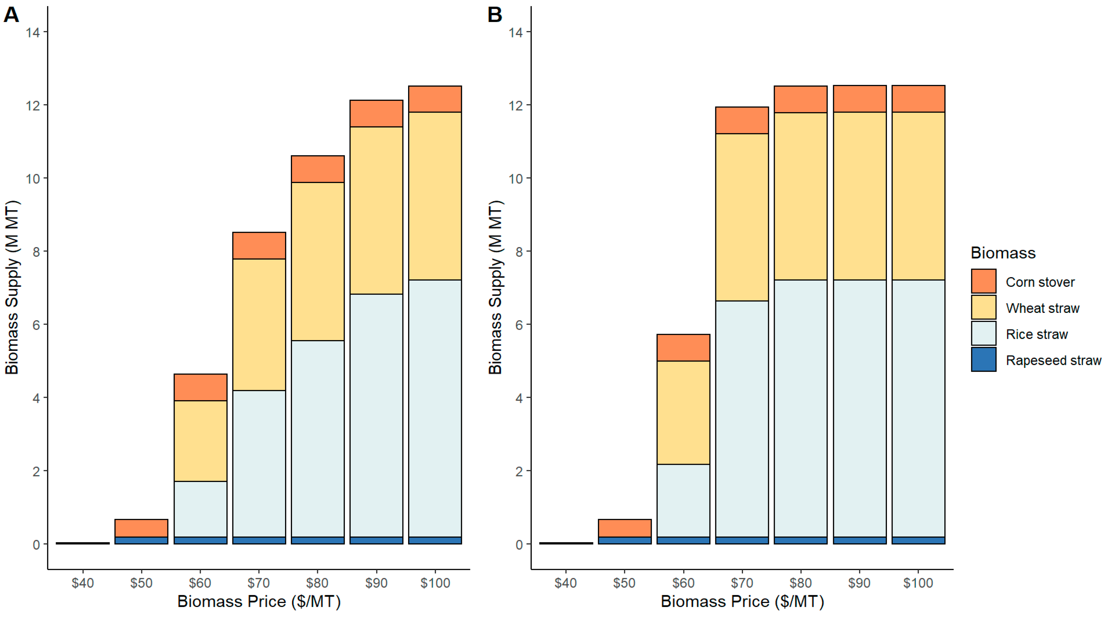
Figure 3 shows the aggregate supply and mix of feedstock that are economically viable for production under various assumptions about biomass prices and co-firing levels. The total biomass supply increases with biomass prices and co-firing levels. Biomass production is economically viable at a minimum price of USD 40/MT. At biomass prices between USD 50 and USD 80/MT, the residue production increases dramatically from 0.7 to 10.6 M MT at a 10% co-firing rate. The scenario with a 20% co-firing rate leads to an increase in biomass production from 0.7 to 12.5 M MT, for the same range of biomass prices. As the biomass price surpasses USD 80/MT, the residue supply response becomes more inelastic in both co-firing scenarios. As shown in Figure 3, once the total residue supply reaches about 12.1 M MT with a 10% co-firing rate or 12.5 M MT with a 20% co-firing rate, the incremental amount of the total residue supply with increasing biomass prices is very marginal under both co-firing scenarios. The unresponsive supply at higher prices is mostly due to the physical residue availability limits. In general, our results align with previous studies on supply patterns. Chen [21] evaluated the economic supply potential of crop residues at the national level and found that the biomass supply is inelastic when the market price is USD 70/MT and above. Similarly, Baker et al. [44] estimated that the supply of logging residues for bioelectricity generation is inelastic at USD 60–80/MT in the US.

The mix of feedstocks produced varies with the biomass prices and co-firing levels. The supply of rapeseed straw and corn stover is dominant at lower biomass prices (≤USD 50/MT). As the biomass price and co-firing rate increase, two high yielding but costly residues, wheat straw and rice straw, comprise a large share of the feedstock portfolio. At a 10% co-firing rate, when the biomass price increases from USD 60/MT to USD 100/MT, the amounts of wheat straw and rice straw increase substantially from 2.2 M MT to 4.6 M MT and from 1.5 M MT to 7.0 M MT, respectively. At a 20% co-firing rate, the amounts of wheat straw and rice straw increase from 2.8 M MT to 4.6 M MT and from 2.0 M MT to 7.0 M MT, respectively, for the same range of biomass prices. The share of rice straw increases from 33% to 56% of the total biomass supply, while the share of wheat straw decreases from 47% to 37% of the total biomass production, when the biomass price increases from USD 60/MT to USD 100/MT. A similar trend for rice straw and wheat straw is found with a 20% co-firing rate.

5.2. Spatial Distribution of Crop Residues and Logistics

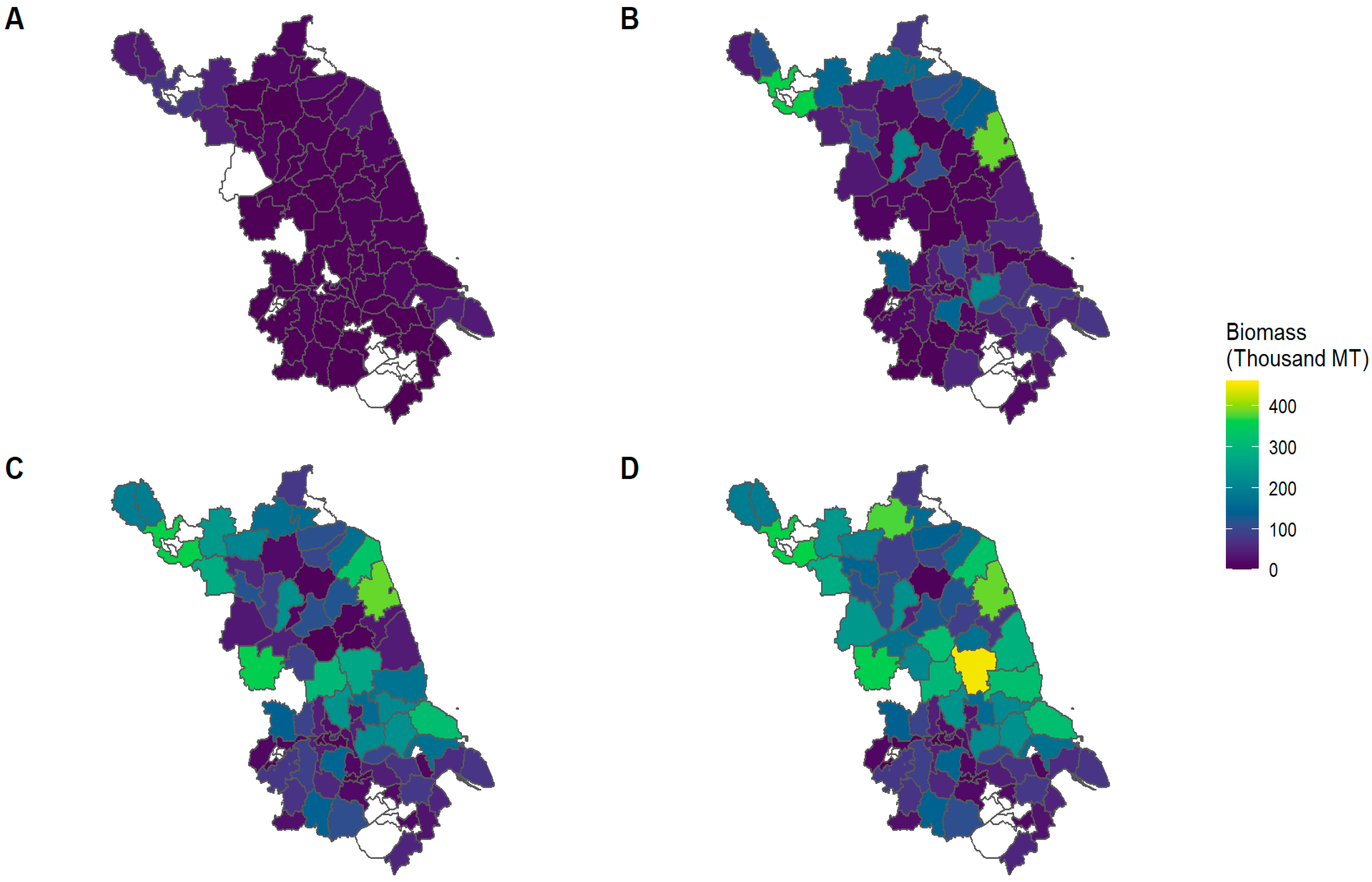
The spatial distribution of feedstock production at the county level for four different price levels (USD 50–USD 80/MT) at a 10% co-firing rate is shown in Figure 4. The heterogeneity of the yields and production costs of crop residues as well as the cropland availability drive the variability in feedstocks distribution across the province. At lower biomass prices (USD 50/MT), the available biomass feedstocks are sourced from corn stover and rapeseed straw and are mainly concentrated in the eastern (e.g., Yancheng and Nantong) and northern regions (e.g., Xuzhou). Many counties show a very limited supply of biomass until the biomass prices approach USD 60/MT. The northern and central counties join the feedstocks supply network at biomass prices of USD 60/MT, mainly because they are the main producers of wheat and rice straws. The extensive margin of crop residues production expands into new counties at higher biomass prices (>USD 70/MT). At these prices, a strong concentration of the supply potential is found around cities with relatively high levels of rice and wheat production activity (e.g., Yancheng, Huai’an, Xuzhou, Suqian, etc.). These regions account for about 53% of the total biomass supply. The corresponding county-level analysis of a 20% co-firing rate indicates a similar spatial distribution pattern across biomass price scenarios (see Figure S1). In general, the regional supply of residues is expected to vary with the biomass prices. At lower biomass prices, the supply of residues is concentrated in the eastern part of the province, while higher biomass prices incentivize the collection of larger amounts of biomass feedstocks from the northern and central parts of the province.

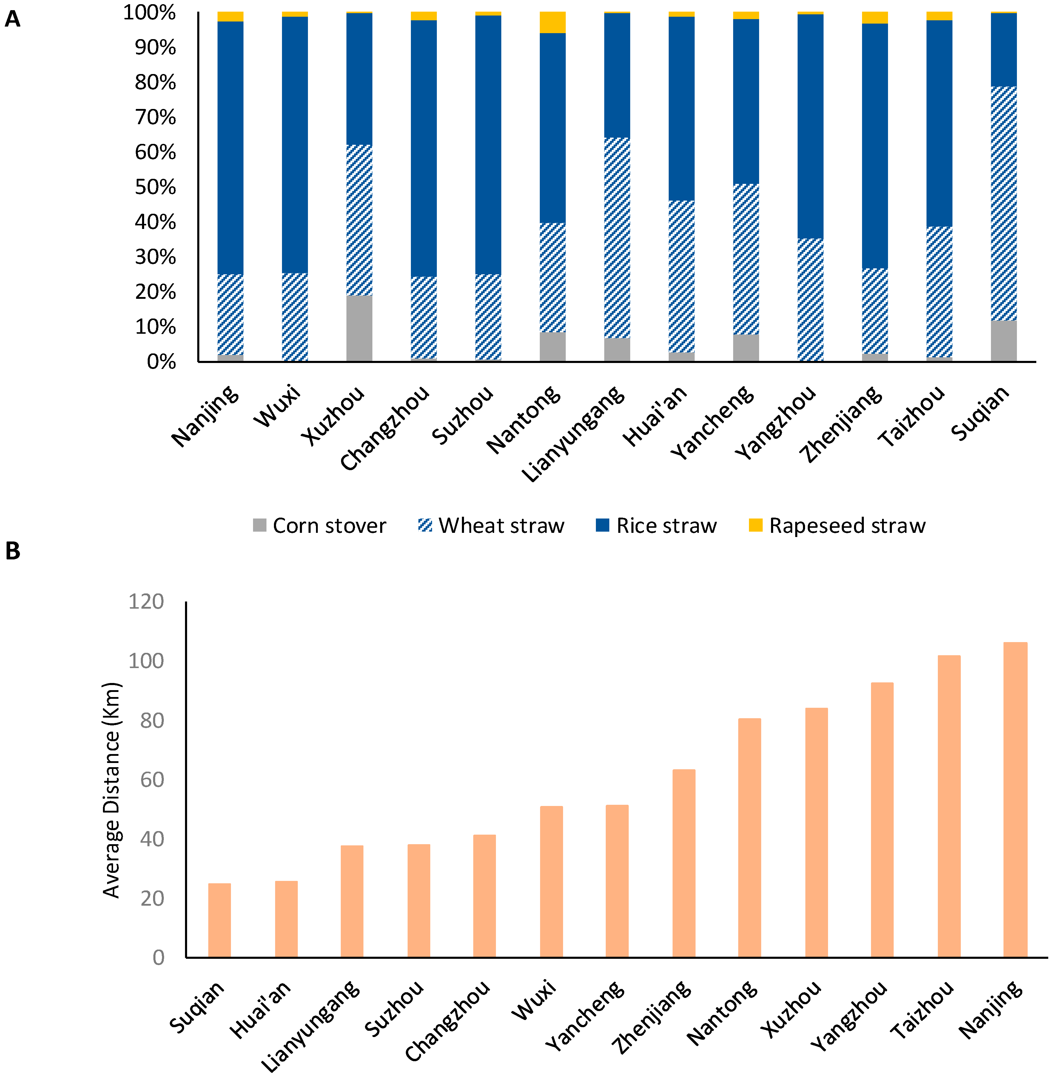
We also estimated the economic biomass supply and average biomass hauling distances for the bioelectricity facilities located in the 13 investigated cities. Our modeling results suggest that there are large variations in the economic biomass supply and logistics across the 13 cities (see Figure 5). For instance, at a biomass price of USD 80/MT, rice straw and wheat straw are the two major feedstocks, representing on average 52% and 38% of the total biomass supply at a 10% co-firing rate, respectively.

For the co-firing facilities located in Suzhou, Wuxi, Changzhou, and Nanjing, rice straw represents more than 70% of the total biomass supply. Rice straw dominates the biomass supply in all 13 cities except for at the facilities located in Lianyungang, Xuzhou, and Suqian, partly because rice production is less prevalent in these cities. A similar dominant share of rice straw (61%) and wheat straw (33%) in the total biomass supply is found at a 20% co-firing level (Figure S2). We also estimate the average hauling distance (weighted by the amount of biomass supplied to the power plant) during the transporting process, finding that the average hauling distance (one-way) ranges from 25 to 106 km at the biomass price of USD 80/MT and a 10% co-firing rate. The shortest hauling distance is found in Suqian, while the longest hauling distance is found in Nanjing. This is due to the regional differences in residue availability and accessibility. A higher co-firing rate is found to reduce the provincial average hauling distance by 21%, as facilities can source more biomass from regions that are closer to their location with a released co-firing constraint.

5.3. GHG Implications

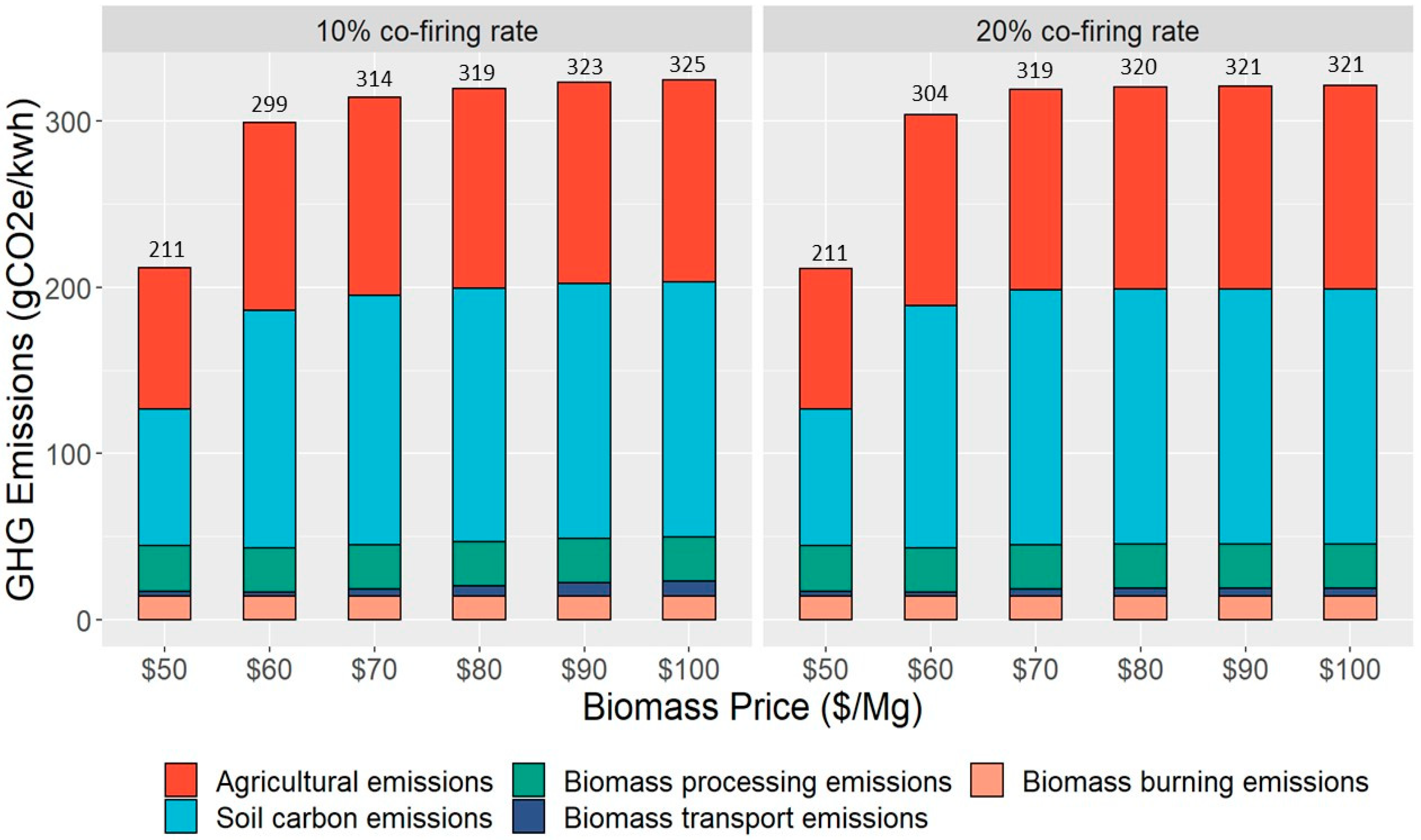
We used the mathematical programming model for co-fired biomass production combined with the life cycle emissions to calculate the GHG emissions with residue-based electricity generation under various biomass price scenarios at two co-firing rate levels. Instead of reporting the absolute GHG emissions, reporting emissions per kWh of electricity makes a clearer comparison with coal-based electricity. As shown in Figure 6, the total GHG emissions increase with an increase in biomass price and range between 211 and 325 g CO₂e/kWh for the USD 50–USD 100/MT range of the biomass price with a 10% co-firing rate. The corresponding estimate of the GHG emissions with a 20% co-fired biomass range is between 211 and 321 g CO₂e/kWh, for the same range of the biomass price. The total GHG emissions are broken down into several components based on the different stages of bioelectricity generation. Removal of crop residues from fields leads to a soil carbon loss. The net GHG emissions associated with soil carbon change were estimated to range between 82 and 153 g CO₂e/kWh for a USD 50–USD 100/MT biomass price with a 10% co-firing rate. The GHG emission associated with agricultural production includes the emission incurred from feedstock production at the farm gate. This was calculated by multiplying the energy use in the planting, maintaining, and harvesting of residues and row crops (relative to the zero-biomass price case) by the corresponding emission factors (in g CO₂e per unit of energy input). The emissions in this sector vary between 85 and 122 g CO₂e/kwh for a USD 50–USD 100/MT biomass price. The emissions from biomass processing contributed about 27 g CO₂e/kwh across all price scenarios, representing 9% of the total emissions. The changes in the soil organic carbon and above-ground emissions during the biomass-producing process are key determinants of the overall GHG emissions of bioelectricity; together, they contribute about 86% of the total GHG emissions. The GHG emissions from biomass transportation increase with the biomass price, as fuel consumption (i.e., diesel) increases with a longer transportation distance. They range between 3.1 and 9.1 g CO₂e/kwh at a biomass price of USD 50–USD 100/MT. The last stage is burning biomass for electricity generation, which results in 13.9 g CO₂e/kwh emissions to the atmosphere. It is worth noting that we assume that the carbon content in residue biomass is biogenic and, therefore, carbon-neutral, which is consistent with the existing literature [44,46]. The GHG emissions under a 20% co-firing rate scenario show a very similar proportion for each sector (Figure 6). Our findings are consistent with the results from prior studies, which showed that the GHG emissions of crop-residue-based electricity range between 235 and 325 g CO₂e/kwh [23,46]. As a reference, the GHG emissions for China’s coal-fired and natural-gas-fired electricity were about 1230 g CO₂e/kwh and 856 g CO₂e/kwh, respectively [45]. In general, the results affirm that biopower leads to substantially lower GHG emissions than fossil-fuel-based electricity.

5.4. Social Benefits of Biomass Co-Firing

We estimated the social benefits of biomass co-firing in coal power plants regarding coal replacement, biomass producers’ surplus, and GHG savings. As indicated in

Table 1. GHG emissions and net GHG savings with various levels of biomass prices and co-firing rates.

	Biomass Price	Coal Replacement (1000 MT)	Agricultural Producer Surplus (USD M)	GHG Emissions (M MT CO2e)
				Emissions from Coal-Based Electricity (a)	GHG Avoided from Coal Displacement (b)	Emissions from Biopower (c)	Emissions from Biomass Open Burning (d)	Net GHG Savings (e) = (b) − (c) + (d)
10% Co-firing	USD 0	0	4244.02	426.97	0	0	0	0
	USD 50	534.77	4246.53	423.51	3.46	0.27	0.05	3.24
	USD 60	3765.93	4260.70	402.61	24.36	2.71	0.39	22.03
	USD 70	6914.94	4330.41	382.24	44.73	5.23	0.71	40.21
	USD 80	8621.44	4424.91	371.20	55.76	6.63	0.88	50.02
	USD 90	9854.93	4539.22	363.23	63.74	7.67	1.01	57.09
	USD 100	10,172.83	4655.14	361.17	65.80	7.95	1.04	58.89
20% Co-firing	USD 0	0	4244.02	426.97	0	0	0	0
	USD 50	534.95	4246.54	423.51	3.46	0.27	0.05	3.24
	USD 60	4643.43	4262.49	396.93	30.03	3.40	0.48	27.11
	USD 70	9703.62	4353.37	364.20	62.76	7.45	0.99	56.31
	USD 80	10,172.06	4471.45	361.17	65.79	7.85	1.04	58.99
	USD 90	10,175.59	4584.44	361.15	65.82	7.86	1.04	59.00
	USD 100	10,176.15	4706.89	361.15	65.82	7.86	1.04	59.00

, coal replacement varies from 0.5 to 10.2 M MT for the biomass price range of USD 50–USD 100/MT with a 10% co-firing rate. A 20% co-firing rate leads to an average of 18% more coal replacement (relative to the case with a 10% co-firing rate) over all biomass price levels. At relatively higher biomass prices (≥USD 80/MT) and a 20% co-firing rate, the amount of coal replacement does not change significantly along with the biomass prices, mainly due to the physical limits of the biomass supply. Our welfare analysis shows that an increased biomass demand for co-firing has very modest effects on food crop prices and the agricultural consumers’ surplus. However, agricultural producers are better off compared to the case with the zero-biomass price. The total surplus gained by the agricultural producers increases by 10% (relative to the zero-biomass price) and reaches about USD 4655 M at a 10% co-firing level when the biomass price is as high as USD 100/MT. A 20% co-firing rate leads to an average of a 1% additional gain in the producers’ surplus than that under a 10% co-firing level over all biomass price scenarios, with the highest surplus of USD 4707 M obtained at a USD 100/MT biomass price. We calculated the net GHG savings with biomass co-firing power generation given various biomass prices and co-firing rates. The GHG savings is measured by the avoided GHG emissions with electricity production due to coal replacement plus the avoided emissions from open burning, the net of the life cycle emissions generated during the process of feedstock production, transportation, and the conversion to bioelectricity. We present the absolute GHG emissions under various alternative scenarios and the total savings by making a comparison with the GHG emissions under the zero-biomass price (or 100% coal). The emission from coal-based electricity is highest (427 M MT CO₂e) at the zero-biomass price, i.e., with no coal replacement. The avoided GHG emissions show an upward trend along with an increasing amount of coal replacement. Moderate differences in the total avoided GHG emissions are found between the two co-firing scenarios at a given biomass price of USD 50-USD 60/MT. Higher levels of the biomass price and co-firing rate lead to a greater amount of GHG savings, with the largest mitigation potential (59 M MTCO₂e) achieved at the highest biomass price of USD 100/MT and a 20% co-firing rate. Overall, biomass co-firing electricity provides 0.8–13.8% (3.2–59 M MTCO₂e) GHG savings relative to coal-based electricity.

5.5. Sensitivity Analysis

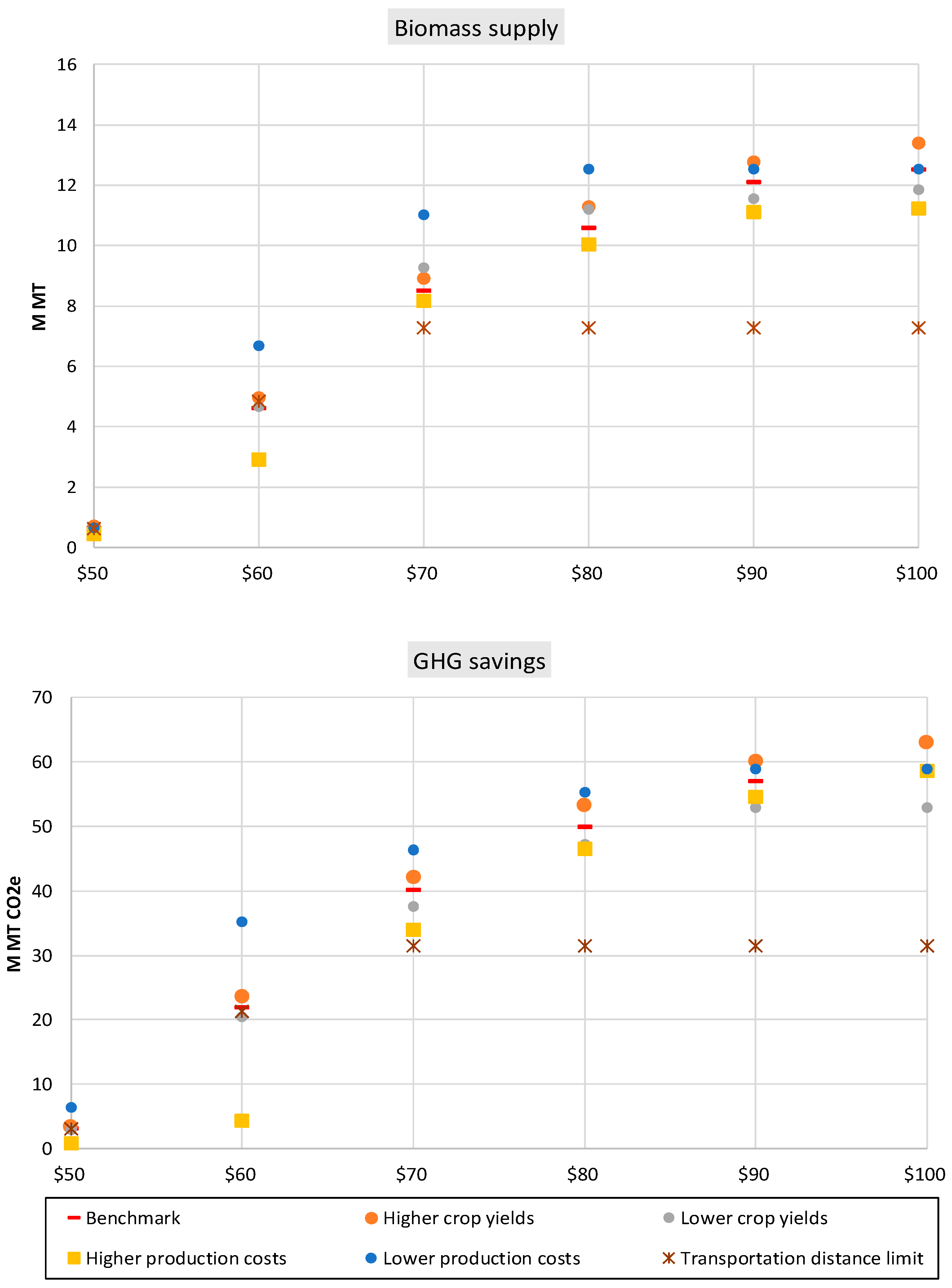
We examined the sensitivity of our findings to several key parameters that affect the productivity of the land, the ease of residue collection, and transportation. Specifically, we considered the effects of major crop yields (corn, rice, wheat, and rapeseed) at ±10% of the benchmark level. We also examined the sensitivity results with 10% higher and lower production costs for the crop residues. Additionally, we considered the possibility that the feedstock transportation distance is no more than 75 km (one way). We found that the biomass supply is most sensitive to assumptions about the crop residue production costs, crop yields, and transportation distance (Figure 7). The effects of these parameters are not uniform across all the biomass price levels. At the relatively lower biomass prices of USD 50–USD 80/MT, a 10% increase in residue production costs (including the costs of extra fertilizer, collection, and processing) could lead to a 5% to 37% decrease in the biomass supply, while a 10% decrease in the residue production costs could increase the biomass supply by 18% to 44% relative to the benchmark case. At the relatively higher biomass prices of USD 90–USD 100/MT, the biomass availability is most sensitive to crop yields and transportation distance; a 10% higher crop yield increases the amount of the biomass supply by 5% to 7%, while the inclusion of a restriction on transportation distance decreases the biomass supply by 38% to 42%. The total economic supply potential is estimated to range between 0.4 and 13.4 M MT across all sensitivity scenarios.

We also examined the sensitivity of the GHG savings of biomass co-firing in coal power plants to the same set of key parameters (Figure 7). Our results indicate that the GHG savings are sensitive to alternative assumptions about these parameters. Uncertainties in key parameters expand the estimated range of GHG savings from 3.2–59 M MT CO2e to 0.8–63 M MT CO₂e across all the biomass price levels. At relatively lower biomass prices (USD 50–USD 80/MT), the GHG savings are most sensitive to the assumption of residue production costs; a 10% decrease in the production cost increases the GHG savings by 25% to 60%. At relatively higher biomass prices (USD 90–USD 100/MT), the GHG savings are most sensitive to assumptions about crop yields and transportation distance. We found that a 10% higher yield of crops leads to a 4–9% increase in GHG savings, while a transportation distance limitation decreases the GHG savings by 44–46%.

Our sensitivity analysis indicates that plausible improvements in crop yields and a reduction in biomass production costs would result in more supply potential and GHG mitigation benefits. Transportation distance is also an impactful factor in determining the biomass availability for co-firing with coal at the power plants. Our results further demonstrate that a correct account of the transportation distance and associated cost is important for evaluating the biomass supply and GHG mitigation potential. An arbitrary assumption of the transportation distance or a buffer-zone-based approach ignoring the real road conditions may bias the estimation results.

6. Discussion

The challenges of balancing economic growth and environmental sustainability have been on the rise in China, particularly among the most economically developed provinces such as Jiangsu. Coal–biomass co-firing generation has been promoted by the state government in a series of political documents (e.g., the National 13th Five-Year Plan). However, its development has been much slower in recent years than that of other renewable energies, such as solar and wind power, largely due to policy uncertainty. State and local governments usually hesitate to keep promoting large-scale biomass co-firing because of the unstable biomass supply and induced land-use change issues that may threaten food security. In contrast to previous studies focusing on the technical supply potential of residue-based biomass [17], our results indicate that biomass prices of USD 50/MT would be required to incentivize farmers to collect crop residues and supply them for biopower purposes. About 12.5 M MT of biomass is economically viable when the price is as high as USD 100/MT, with 56% of biomass being rice straw. Our results for the maximum feasible biomass supply are substantially smaller than the theoretical potential estimated by previous studies, which overlooked the economic incentives and co-firing capacity, and are comparable with the estimated sustainable potential (15 M MT) by [17].

Our spatial allocation framework goes beyond previous national or subnational studies by offering a detailed picture of the supply potential at the county level. Coal-fired power plants are unevenly distributed in Jiangsu, with most of them located in the southern industrial area, while the major residue production counties are located in the northern agricultural area. Spatial analysis has several practical implications. First, the spatial distribution map of the biomass supply provides valuable insights for any counties and facilities interested in evaluating the potential biomass co-firing pathways. Second, power plants in the province could make an informed decision about selecting appropriate feedstock with minimum costs. Third, given the geographic mismatch between the biomass supply and demand sites, it is ideal to establish some processing stations in the central region (e.g., in Yangzhou, Taizhou, and Nantong); thus, the abundant residues produced in the northern agricultural counties can be preprocessed and stored there and then redistributed to the power plants located in the southern area. In addition, it might be more profitable for some power plants to source biomass from neighbor provinces, such as Anhui, if interprovince transportation is considered.

The direct biomass co-firing technology has reached maturity and been commercialized in several power plants in China. For instance, Xinyuan Power Generation Co., Ltd. of Xuzhou, Jiangsu and Baoyin Power Generation Co., Ltd. of Yangzhou, Jiangsu operate with up to 20% biomass co-firing. Despite the technological readiness, the generation efficiency of biomass co-firing is generally low [10]. The high cost of raw biomass and insufficient subsidies are the main handicaps for large-scale application. In this study, we explore the economic potential of biomass co-firing in existing power plants, assuming they are equally eligible to utilize any biomass. It should be noted that this treatment might overestimate the biomass demand, given that newer and bigger plants would be less likely to burn biomass with coal [54].

Our study has several policy implications. It shows the condition under which agricultural residues have the potential to offer climate benefits and would warrant policy support. At present, Jiangsu provides subsidies ranging from USD 25–USD 35/MT (depending on the residue production region) to encourage farmers to retain crop residues [55]. Our results show that this subsidy needs to be doubled to make crop residues economically viable for electricity generation. A well-designed subsidization scheme can incentivize farmers to supply a reasonable quantity of residues to power plants without harming soil nutrients. Our life cycle assessment of bioelectricity GHG emissions indicates that agricultural and soil carbon emissions are the two main contributors to net GHG emissions. Policies aimed at reducing chemical fertilizer usage and encouraging more sustainable land management activities, such as conservative tillage and fallowing the land, can increase carbon benefits. Our social welfare analysis shows that bioelectricity leads to an increase in agricultural producers’ surplus. Policies promoting local bioenergy development can contribute to rural development and alleviate poverty. Lastly, our results from this analysis can provide more accurate and region-specific biomass supply curve information. Such information can advance the depiction of biomass cost curves in the current bottom-up simulation models (e.g., energy sector models and integrated assessment models) and result in a more robust analysis of renewable energy policies.

7. Conclusions

The decision to partially replace coal with biomass to generate electricity requires scrutiny on both the economic and environmental dimensions. In this paper, we developed a partial equilibrium model to comprehensively assess the economic potential of crop residues’ co-firing with coal and the accompanying environmental effects in Jiangsu. We found that the viable biomass for co-firing in coal-based power plants is 0.7–12.5 M MT at biomass prices between USD 50 and USD 100/MT. Up to 20% biomass co-firing can replace the maximum of 10.2 M MT of coal when the biomass price is as high as USD 100/MT. Agricultural producers are better off by USD 463 M at a biomass price of USD 100/MT, relative to the case with the zero-biomass price. Our investigation of the economic supply potential of biomass and the associated social benefits can inform the design of policy interventions to promote bioenergy and alleviate rural poverty.

The potential for GHG savings with biopower generation is found to be 59 M MMT CO₂e with a USD 100/MT biomass price, which affirms that biomass–coal co-firing electricity generation can make a substantive contribution to GHG mitigation. Our results have implications for developing low-carbon policies (e.g., a carbon tax) to supplement market-based incentives for bioelectricity production if the biomass price is too low.

Although this analysis does not project future changes in the crop residues supply, the implied range of the supply potential under various market conditions provides a meaningful range for the expected future biomass availability. We expect this research to be helpful when making informed decisions related to low-carbon energy transition, particularly in some hotspot provinces of China such as Jiangsu, Shandong, and Hennan, which were identified as favorable provinces for crop-residue-based bioenergy development.

Furthermore, programs promoting biomass utilization at existing coal-fired powerplants could result in higher production costs, which may impede power producers from co-firing biomass. In this study, we focus our assessment on the agricultural sector and ignore the potential effects of the electricity market. To inform the sustainable utilization of biomass resources, the proposed model could be extended to include the electricity sector. In addition, more research is necessary to address the environmental effects, such as on biodiversity and water usage, in a broader manner. We leave these explorations to future work.

References

1. Yang, H.; Huang, X.; Hu, J.; Thompson, J.R.; Flower, R.J. Achievements, Challenges and Global Implications of China’s Carbon Neutral Pledge. Front. Environ. Sci. Eng. 2022, 16, 111. [Google Scholar] [CrossRef] [PubMed]
2. National Energy Administration. National Renewable Energy Power Development Monitoring and Evaluation Report. 2021. Available online: http://www.nea.gov.cn/2022-09/16/c_1310663387.htm (accessed on 26 November 2022). (In Chinese)
3. Cui, R.Y.; Hultman, N.; Cui, D.; McJeon, H.; Yu, S.; Edwards, M.R.; Sen, A.; Song, K.; Bowman, C.; Clarke, L.; et al. A Plant-by-Plant Strategy for High-Ambition Coal Power Phaseout in China. Nat. Commun. 2021, 12, 1468. [Google Scholar] [CrossRef] [PubMed]
4. Liu, J.; Wang, Q.; Song, Z.; Fang, F. Bottlenecks and Countermeasures of High-Penetration Renewable Energy Development in China. Engineering 2021, 7, 1611–1622. [Google Scholar] [CrossRef]
5. Lu, X.; Cao, L.; Wang, H.; Peng, W.; Xing, J.; Wang, S.; Cai, S.; Shen, B.; Yang, Q.; Nielsen, C.P.; et al. Gasification of Coal and Biomass as a Net Carbon-Negative Power Source for Environment-Friendly Electricity Generation in China. Proc. Natl. Acad. Sci. USA 2019, 116, 8206–8213. [Google Scholar] [CrossRef] [Green Version]
6. IEA. An Energy Sector Roadmap to Carbon Neutrality in China; OECD Publishing: Paris, France, 2021. [Google Scholar]
7. National Bureau of Statistics of China. China Energy Statistical Yearbook. 2021. Available online: Https://Data.Cnki.Net/Trade/Yearbook/Single/N2021050066?Zcode=Z023 (accessed on 3 December 2022).
8. Zhang, Q.; Zhou, D.; Zhou, P.; Ding, H. Cost Analysis of Straw-Based Power Generation in Jiangsu Province, China. Appl. Energy 2013, 102, 785–793. [Google Scholar] [CrossRef]
9. Netherlands Enterprise Agency. Sector Report Biomass Energy in Jiangsu Province. 2015. Available online: Www.Rvo.Nl. (accessed on 19 January 2023).
10. Xu, Y.; Yang, K.; Zhou, J.; Zhao, G. Coal-Biomass Co-Firing Power Generation Technology: Current Status, Challenges and Policy Implications. Sustainability 2020, 12, 3692. [Google Scholar] [CrossRef]
11. Nguyen, T.H.; Field, J.L.; Kwon, H.; Hawkins, T.R.; Paustian, K.; Wang, M.Q. A Multi-Product Landscape Life-Cycle Assessment Approach for Evaluating Local Climate Mitigation Potential. J. Clean. Prod. 2022, 354, 131691. [Google Scholar] [CrossRef]
12. Yuan, Y.; Zhao, J. Study on the Supply Capacity of Crop Residue as Energy in Rural Areas of Heilongjiang Province of China. Renew. Sustain. Energy Rev. 2014, 38, 526–536. [Google Scholar] [CrossRef]
13. Shu, K.; Schneider, U.; Scheffran, J. Bioenergy and Food Supply: A Spatial-Agent Dynamic Model of Agricultural Land Use for Jiangsu Province in China. Energies 2015, 8, 13284–13307. [Google Scholar] [CrossRef] [Green Version]
14. Wu, J.; Zhang, J.; Yi, W.; Cai, H.; Li, Y.; Su, Z. Agri-Biomass Supply Chain Optimization in North China: Model Development and Application. Energy 2022, 239, 122374. [Google Scholar] [CrossRef]
15. Xue, S.; Lewandowski, I.; Wang, X.; Yi, Z. Assessment of the Production Potentials of Miscanthus on Marginal Land in China. Renew. Sustain. Energy Rev. 2016, 54, 932–943. [Google Scholar] [CrossRef]
16. Qiu, H.; Sun, L.; Xu, X.; Cai, Y.; Bai, J. Potentials of Crop Residues for Commercial Energy Production in China: A Geographic and Economic Analysis. Biomass Bioenergy 2014, 64, 110–123. [Google Scholar] [CrossRef]
17. Zhang, B.; Xu, J.; Lin, Z.; Lin, T.; Faaij, A.P.C. Spatially Explicit Analyses of Sustainable Agricultural Residue Potential for Bioenergy in China under Various Soil and Land Management Scenarios. Renew. Sustain. Energy Rev. 2021, 137, 110614. [Google Scholar] [CrossRef]
18. Qin, Z.; Zhuang, Q.; Cai, X.; He, Y.; Huang, Y.; Jiang, D.; Lin, E.; Liu, Y.; Tang, Y.; Wang, M.Q. Biomass and Biofuels in China: Toward Bioenergy Resource Potentials and Their Impacts on the Environment. Renew. Sustain. Energy Rev. 2018, 82, 2387–2400. [Google Scholar] [CrossRef]
19. Kang, Y.; Yang, Q.; Bartocci, P.; Wei, H.; Liu, S.S.; Wu, Z.; Zhou, H.; Yang, H.; Fantozzi, F.; Chen, H. Bioenergy in China: Evaluation of Domestic Biomass Resources and the Associated Greenhouse Gas Mitigation Potentials. Renew. Sustain. Energy Rev. 2020, 127, 109842. [Google Scholar] [CrossRef] [PubMed]
20. Xing, X.; Wang, R.; Bauer, N.; Ciais, P.; Cao, J.; Chen, J.; Tang, X.; Wang, L.; Yang, X.; Boucher, O.; et al. Spatially Explicit Analysis Identifies Significant Potential for Bioenergy with Carbon Capture and Storage in China. Nat. Commun. 2021, 12, 3159. [Google Scholar] [CrossRef]
21. Chen, X. Economic Potential of Biomass Supply from Crop Residues in China. Appl. Energy 2016, 166, 141–149. [Google Scholar] [CrossRef]
22. Fang, Y.R.; Shi, W.; Xie, G.H. Implications of Wheat Straw Logistic Systems for Bioenergy Sustainable Development in China: Costs, Energy Consumption, and GHG Emissions. Sci. Total Environ. 2022, 837, 155633. [Google Scholar] [CrossRef] [PubMed]
23. Li, J.; Wang, R.; Li, H.; Nie, Y.; Song, X.; Li, M.; Shi, M.; Zheng, X.; Cai, W.; Wang, C. Unit-Level Cost-Benefit Analysis for Coal Power Plants Retrofitted with Biomass Co-Firing at a National Level by Combined GIS and Life Cycle Assessment. Appl. Energy 2021, 285, 116494. [Google Scholar] [CrossRef]
24. Hudiburg, T.W.; Wang, W.; Khanna, M.; Long, S.P.; Dwivedi, P.; Parton, W.J.; Hartman, M.; DeLucia, E.H. Impacts of a 32-Billion-Gallon Bioenergy Landscape on Land and Fossil Fuel Use in the US. Nat. Energy 2016, 1, 15005. [Google Scholar] [CrossRef]
25. Masum, F.H.; Wang, W.; Colson, G.; Dwivedi, P. Replacing Coal in Georgia’s Power Plants with Woody Biomass to Increase Carbon Benefit: A Mixed Integer Linear Programming Model. J. Environ. Manag. 2022, 316, 115060. [Google Scholar] [CrossRef] [PubMed]
26. Wang, W.; Dwivedi, P.; Abt, R.; Khanna, M. Carbon Savings with Transatlantic Trade in Pellets: Accounting for Market-Driven Effects. Environ. Res. Lett. 2015, 10, 114019. [Google Scholar] [CrossRef]
27. Searchinger, T.; James, O.; Dumas, P.; Kastner, T.; Wirsenius, S. EU Climate Plan Sacrifices Carbon Storage and Biodiversity for Bioenergy. Nature 2022, 612, 27–30. [Google Scholar] [CrossRef] [PubMed]
28. DeCicco, J.M.; Schlesinger, W.H. Reconsidering Bioenergy given the Urgency of Climate Protection. Proc. Natl. Acad. Sci. USA 2018, 115, 9642–9645. [Google Scholar] [CrossRef] [PubMed] [Green Version]
29. Liska, A.J.; Yang, H.; Milner, M.; Goddard, S.; Blanco-Canqui, H.; Pelton, M.P.; Fang, X.X.; Zhu, H.; Suyker, A.E. Biofuels from Crop Residue Can Reduce Soil Carbon and Increase CO2 Emissions. Nat. Clim. Chang. 2014, 4, 398–401. [Google Scholar] [CrossRef] [Green Version]
30. Mandley, S.; Wicke, B.; Junginger, H.; Vuuren, D.; Daioglou, V. Integrated Assessment of the Role of Bioenergy within the EU Energy Transition Targets to 2050. GCB Bioenergy 2022, 14, 157–172. [Google Scholar] [CrossRef]
31. Appiah-Nkansah, N.B.; Li, J.; Rooney, W.; Wang, D. A Review of Sweet Sorghum as a Viable Renewable Bioenergy Crop and Its Techno-Economic Analysis. Renew. Energy 2019, 143, 1121–1132. [Google Scholar] [CrossRef]
32. Nandimandalam, H.; Gude, V.G. Renewable Wood Residue Sources as Potential Alternative for Fossil Fuel Dominated Electricity Mix for Regions in Mississippi: A Techno-Economic Analysis. Renew. Energy 2022, 200, 1105–1119. [Google Scholar] [CrossRef]
33. Agbor, E.; Oyedun, A.O.; Zhang, X.; Kumar, A. Integrated Techno-Economic and Environmental Assessments of Sixty Scenarios for Co-Firing Biomass with Coal and Natural Gas. Appl. Energy 2016, 169, 433–449. [Google Scholar] [CrossRef]
34. Natelson, R.H.; Wang, W.-C.; Roberts, W.L.; Zering, K.D. Technoeconomic Analysis of Jet Fuel Production from Hydrolysis, Decarboxylation, and Reforming of Camelina Oil. Biomass Bioenergy 2015, 75, 23–34. [Google Scholar] [CrossRef] [Green Version]
35. Moioli, E.; Schildhauer, T. Eco-Techno-Economic Analysis of Methanol Production from Biogas and Power-to-X. Ind. Eng. Chem. Res. 2022, 61, 7335–7348. [Google Scholar] [CrossRef]
36. Zetterholm, J.; Bryngemark, E.; Ahlström, J.; Söderholm, P.; Harvey, S.; Wetterlund, E. Economic Evaluation of Large-Scale Biorefinery Deployment: A Framework Integrating Dynamic Biomass Market and Techno-Economic Models. Sustainability 2020, 12, 7126. [Google Scholar] [CrossRef]
37. Hanssen, S.V.; Daioglou, V.; Steinmann, Z.J.N.; Frank, S.; Popp, A.; Brunelle, T.; Lauri, P.; Hasegawa, T.; Huijbregts, M.A.J.; Van Vuuren, D.P. Biomass Residues as Twenty-First Century Bioenergy Feedstock—A Comparison of Eight Integrated Assessment Models. Clim. Chang. 2020, 163, 1569–1586. [Google Scholar] [CrossRef] [PubMed] [Green Version]
38. Pan, X.; Chen, W.; Wang, L.; Lin, L.; Li, N. The Role of Biomass in China’s Long-Term Mitigation toward the Paris Climate Goals. Environ. Res. Lett. 2018, 13, 124028. [Google Scholar] [CrossRef]
39. Chen, X.; Huang, H.; Khanna, M.; Önal, H. Alternative Transportation Fuel Standards: Welfare Effects and Climate Benefits. J. Environ. Econ. Manag. 2014, 67, 241–257. [Google Scholar] [CrossRef]
40. Ekşioğlu, S.D.; Karimi, H.; Ekşioğlu, B. Optimization Models to Integrate Production and Transportation Planning for Biomass Co-Firing in Coal-Fired Power Plants. IIE Trans. 2016, 48, 901–920. [Google Scholar] [CrossRef] [Green Version]
41. Phanphanich, M.; Mani, S. Impact of Torrefaction on the Grindability and Fuel Characteristics of Forest Biomass. Bioresour. Technol. 2011, 102, 1246–1253. [Google Scholar] [CrossRef]
42. Lizotte, P.-L.; Savoie, P.; De Champlain, A. Ash Content and Calorific Energy of Corn Stover Components in Eastern Canada. Energies 2015, 8, 4827–4838. [Google Scholar] [CrossRef] [Green Version]
43. IEA Bioenergy Annual Report 2021. 2022. Available online: Https://Www.Ieabioenergy.Com/Blog/Publications/Iea-Bioenergy-Annual-Report-2021/ (accessed on 17 January 2023).
44. Baker, J.S.; Wade, C.M.; Sohngen, B.L.; Ohrel, S.; Fawcett, A.A. Potential Complementarity between Forest Carbon Sequestration Incentives and Biomass Energy Expansion. Energy Policy 2019, 126, 391–401. [Google Scholar] [CrossRef]
45. Feng, K.; Hubacek, K.; Siu, Y.L.; Li, X. The Energy and Water Nexus in Chinese Electricity Production: A Hybrid Life Cycle Analysis. Renew. Sustain. Energy Rev. 2014, 39, 342–355. [Google Scholar] [CrossRef] [Green Version]
46. Masum, M.F.H.; Dwivedi, P.; Anderson, W.F. Estimating Unit Production Cost, Carbon Intensity, and Carbon Abatement Cost of Electricity Generation from Bioenergy Feedstocks in Georgia, United States. Renew. Sustain. Energy Rev. 2020, 117, 109514. [Google Scholar] [CrossRef]
47. Guo, S. How Does Straw Burning Affect Urban Air Quality in China? Am. J. Agric. Econ. 2021, 103, 1122–1140. [Google Scholar] [CrossRef]
48. Liang, D.; Lu, X.; Zhuang, M.; Shi, G.; Hu, C.; Wang, S.; Hao, J. China’s Greenhouse Gas Emissions for Cropping Systems from 1978–2016. Sci. Data 2021, 8, 171. [Google Scholar] [CrossRef] [PubMed]
49. IPCC. Climate Change 2013: The Physical Science Basis; Cambridge University Press: Cambridge, UK; New York, NY, USA, 2013. [Google Scholar]
50. Graham, R.L.; Nelson, R.; Sheehan, J.; Perlack, R.D.; Wright, L.L. Current and Potential U.S. Corn Stover Supplies. Agron. J. 2007, 99, 1–11. [Google Scholar] [CrossRef]
51. Sheehan, J.; Aden, A.; Paustian, K.; Killian, K.; Brenner, J.; Walsh, M.; Nelson, R. Energy and Environmental Aspects of Using Corn Stover for Fuel Ethanol. J. Ind. Ecol. 2003, 7, 117–146. [Google Scholar] [CrossRef]
52. Lal, R. World Crop Residues Production and Implications of Its Use as a Biofuel. Environ. Int. 2005, 31, 575–584. [Google Scholar] [CrossRef]
53. Malcolm, S. Weaning off Corn: Crop Residues and the Transition to Cellulosic Ethanol. In The Transition to a BioEconomy: Environmental and Rural Development Impacts, Proceedings of the Environmental and Rural Development Impacts Conference, St. Louis, MO, USA, 15–16 October 2008; Farm Foundation: Oak Brook, IL, USA, 2008. [Google Scholar]
54. Liu, Z.; Altman, I.; Johnson, T.G. The Feasibility of Co-Firing Biomass for Electricity in Missouri. Biomass Bioenergy 2014, 69, 12–20. [Google Scholar] [CrossRef]
55. Chen, J.; Gong, Y.; Wang, S.; Guan, B.; Balkovic, J.; Kraxner, F. To Burn or Retain Crop Residues on Croplands? An Integrated Analysis of Crop Residue Management in China. Sci. Total Environ. 2019, 662, 141–150. [Google Scholar] [CrossRef] [Green Version]
56. Argonne National Laboratory. 2020; GREET Model. Available online: https://greet.es.anl.gov (accessed on 1 August 2021).
57. Huang, J.; Jun, Y.; Xu, Z.; Rozelle, S.; Li, N. Agricultural trade liberalization and poverty in China. China Econ. Rev. 2007, 18, 244–265. [Google Scholar] [CrossRef]
58. Jin, Z.; Shah, T.; Zhang, L.; Liu, H.; Peng, S.; Nie, L. Effect of straw returning on soil organic carbon in rice–wheat rotation system: A review. Food Energy Secur. 2020, 9. [Google Scholar] [CrossRef] [Green Version]
59. Obnamia, J.A.; Dias, G.M.; MacLean, H.L.; Saville, B.A. Comparison of U.S. Midwest corn stover ethanol greenhouse gas emissions from GREET and GHGenius. Appl. Energy 2019, 235, 591–601. [Google Scholar] [CrossRef]
60. WDNR. Forest Biomass and Air Emission. Washington State Department of Natural Resources. 2010. Available online: https://www.dnr.wa.gov/Publications/em_forest_biomass_and_air_emissions_factsheet_7.pdf. (accessed on 24 January 2023).
61. Zhao, L.; Ou, X.; Chang, S. Life-cycle greenhouse gas emission and energy use of bioethanol produced from corn stover in China: Current perspectives and future prospectives. Energy 2016, 115, 303–313. [Google Scholar] [CrossRef]
Figure 1. Flow of information within the model.
Energies 16 02725 g001
Figure 2. Location and capacity (unit: MW) of coal power plants in Jiangsu Province.
Energies 16 02725 g002
Figure 3. Supply and mix of feedstock under alternative scenarios of biomass prices and co-firing rates: (A) 10% co-firing rate; (B) 20% co-firing rate.
Energies 16 02725 g003
Figure 4. Spatial distribution of feedstock production for alternative levels of biomass price with a 10% co-firing rate: (A) USD 50/MT; (B) USD 60/MT; (C) USD 70/MT; (D) USD 80/MT.
Energies 16 02725 g004
Figure 5. Biomass supply mix and average biomass hauling distances by facilities located in 13 cities at USD 80/MT biomass price and 10% co-firing rate: (A) Supply mix of biomass by city; (B) Average biomass transportation distance by city.
Energies 16 02725 g005
Figure 6. GHG emissions of biopower generation by sector.
Energies 16 02725 g006
Figure 7. Total biomass supply and net GHG savings for each sensitivity scenario.
Energies 16 02725 g007