
Identification Efficiency in Dynamic UHF RFID Anticollision Systems with Textile Electronic Tags

 , ,
, ,  , and
, and
Abstract
1. Introduction
1.1. State-of-the-Art
1.2. Research Idea
2. Assumptions for Synthesis
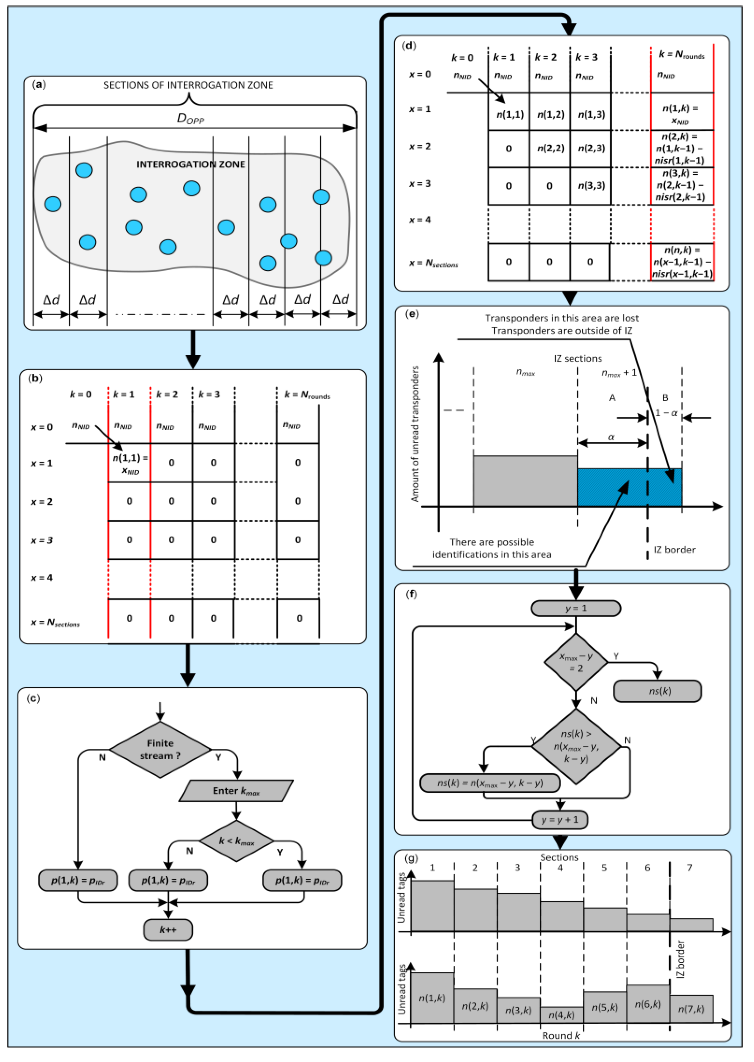
2.1. Numerical Model
- Transponders in the IZ are subjected to identification in a given inventory round;
- The probability of tag recognition does not depend on its location in the IZ;
- The number of unread transponders in a moving group decreases over time as a result of performed identifications;
- The number of transponders read in a round and section is proportional to the number of previously unread tags in that section.
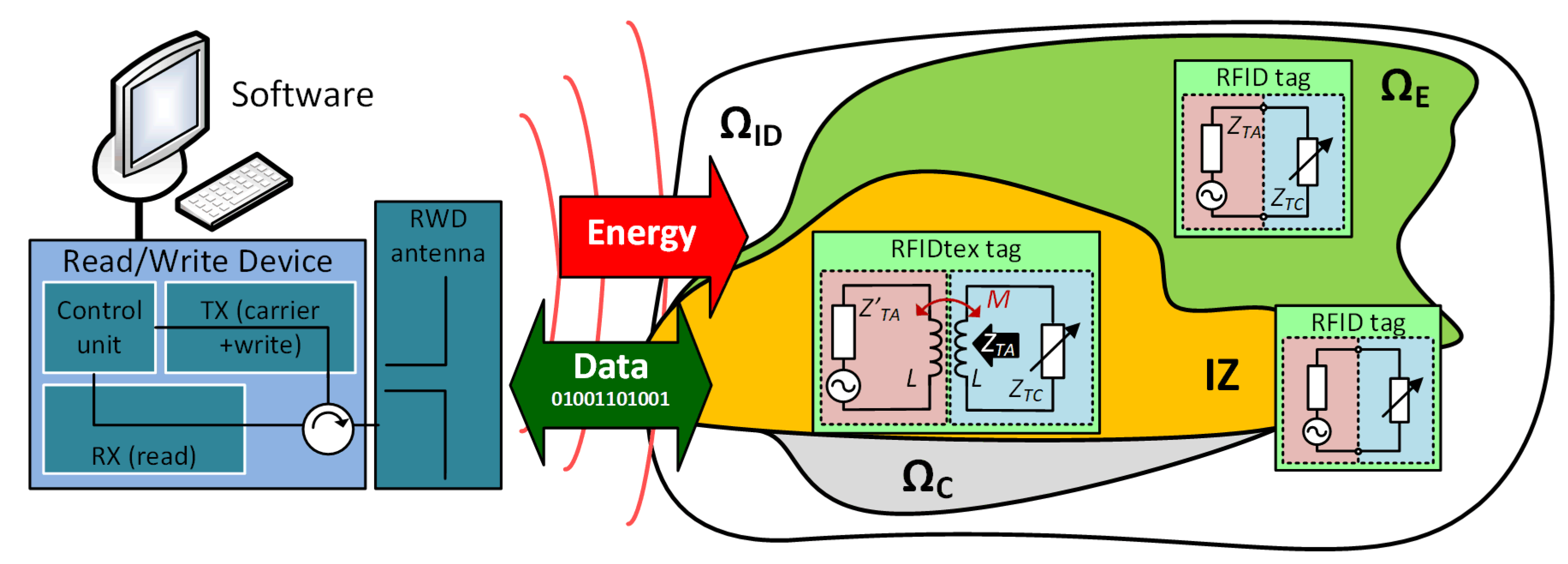
- P with terms p(n,k), equals number of tags unread in section n and round k;
- PISR with terms pisr(n,k), equals number of correct identifications in section n and round k;
- PIR with terms pir(k), equals number of identifications in IZ in round k;
- PS with terms ps(k), equals number of tags lost in round k, tags that have not yet been read.
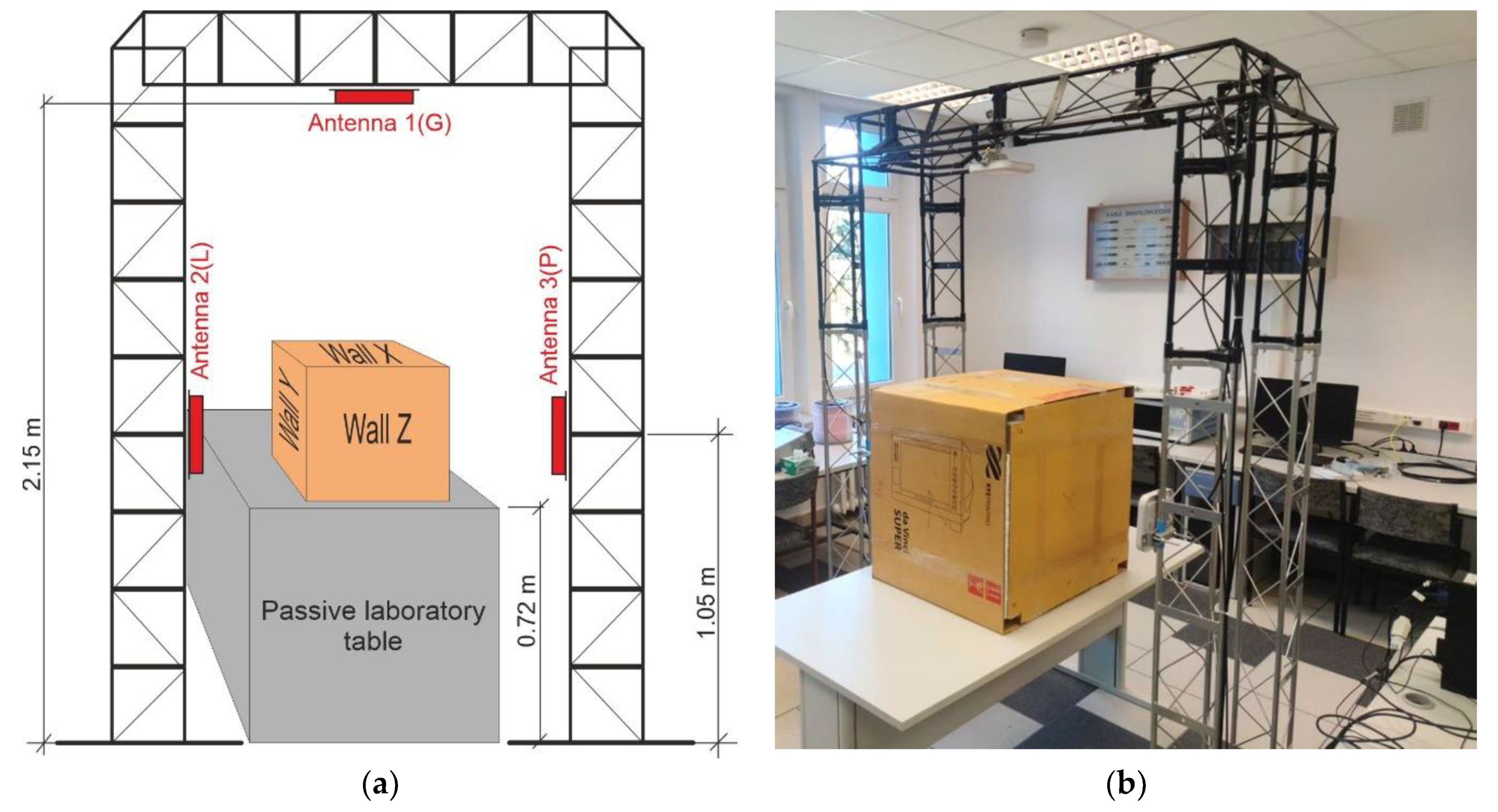
2.2. Conception of Laboratory IoTT Stand
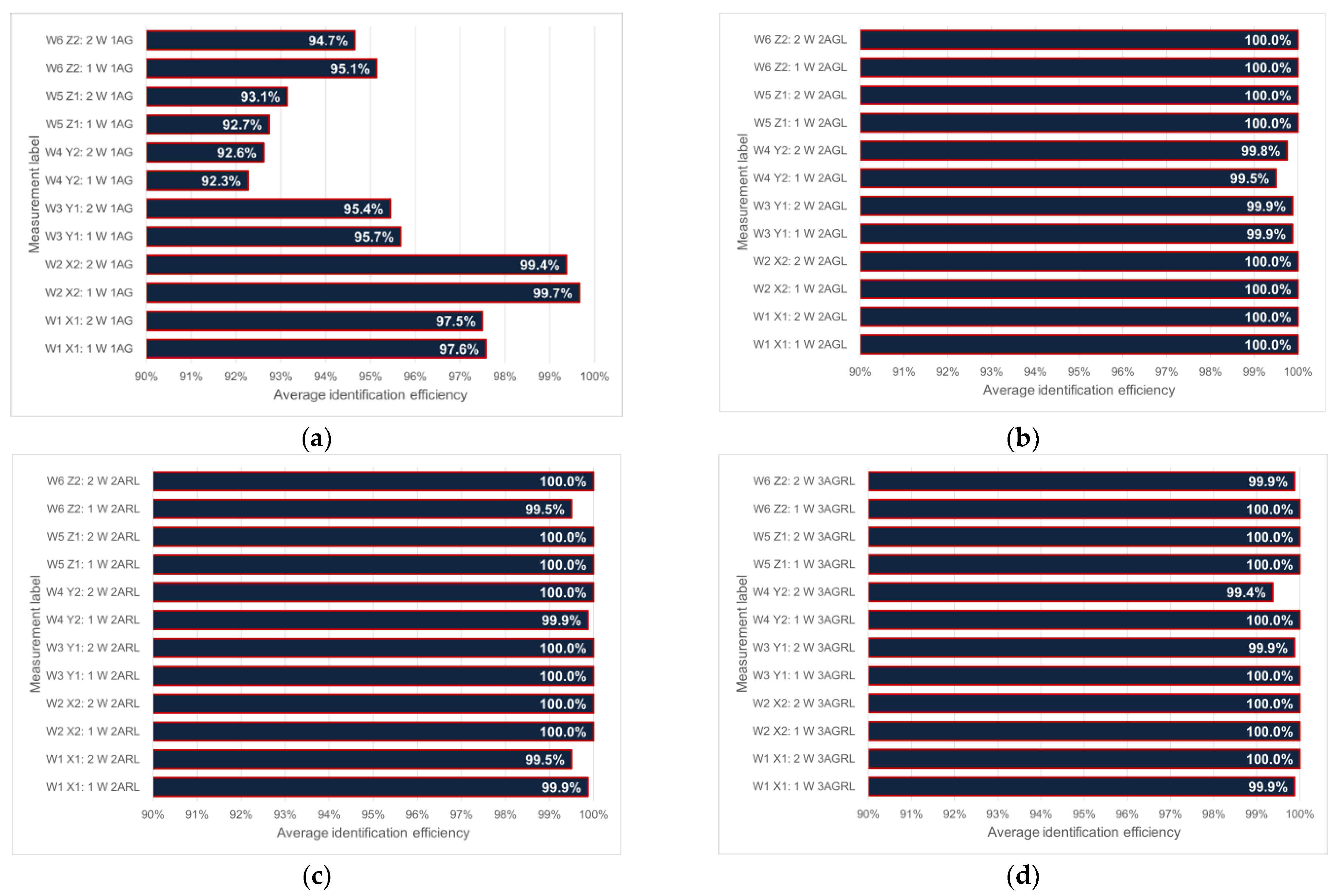
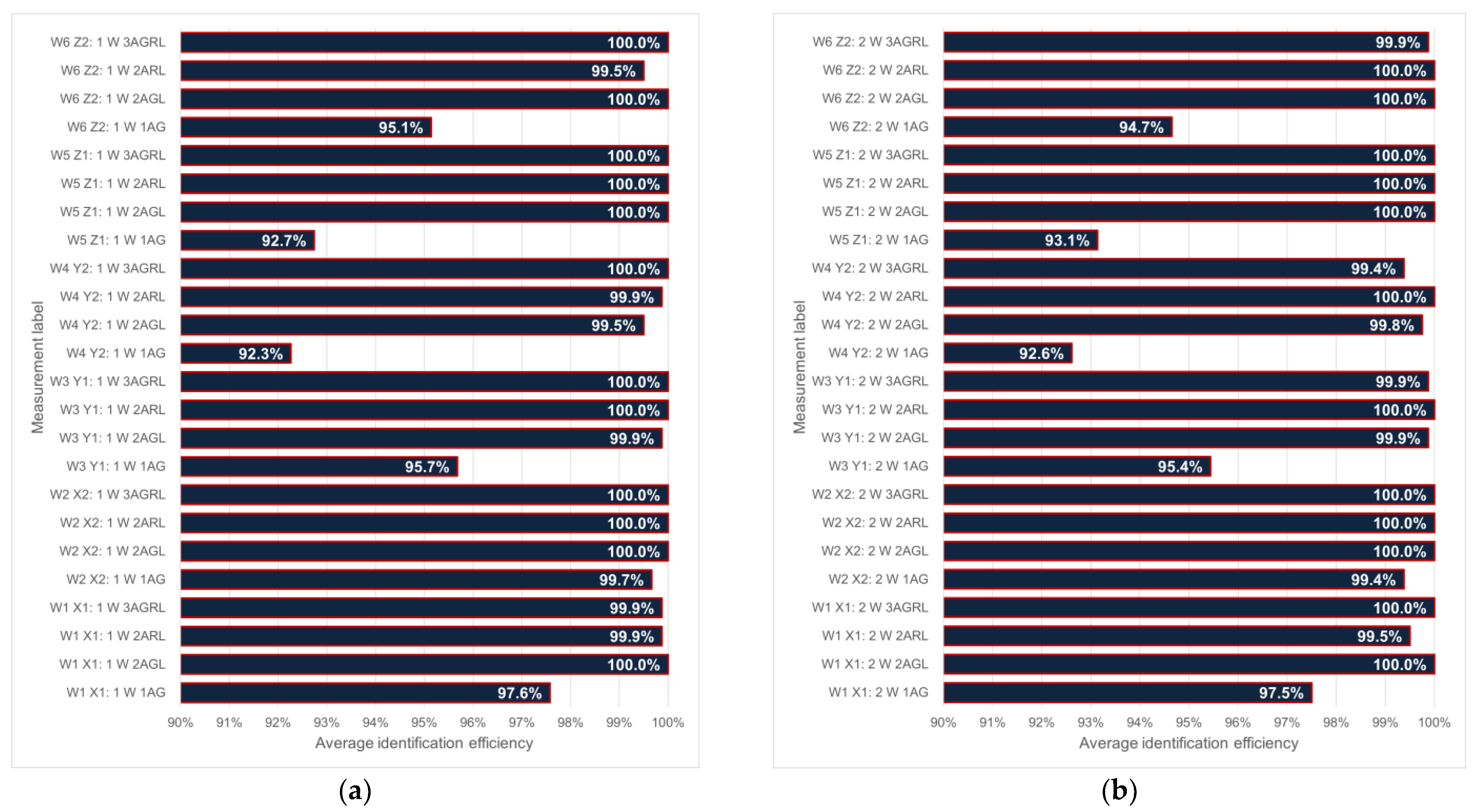
- 1AG—one upper antenna with number 1(G);
- 2AGL—two antennas, upper with number 1(G) and left side with number 2(L);
- 2ALR—two antennas, left side with number 2(L) and right side with number 3(R);
- 3AGLR—three antennas are active.
- W1 X1—wall X is set against the antenna 1(G), wall Z against 2(L) => 1X/2Z
- W2 X2—wall X is set against the antenna 1(G), wall Y against 2(L) => 1X/2Y
- W3 Y1—wall Y is set against the antenna 1(G), wall X against 2(L) => 1Y/2X
- W4 Y2—wall Y is set against the antenna 1(G), wall Z against 2(L) => 1Y/2Z
- W5 Z1—wall Z is set against the antenna 1(G), wall X against 2(L) => 1Z/2X
- W6 Z2—wall Z is set against the antenna 1(G), wall Y against 2(L) => 1Z/2Y.
3. Results
3.1. Dependence of Identification Efficiency on the Number of Objects—Simulation Results
- transmission coding technique: FM0 and Miller for M = 4 and M = 8; M means how many BLF frequency periods there are per bit of transmitted data;
- backscatter link frequency BLF: 40, 160 and 640 kHz;
- maximal duration of inventory round Tmax: 0.1 s, 0.5 s and 1 s;
- persistence time of transponder: 1 s and infinity.
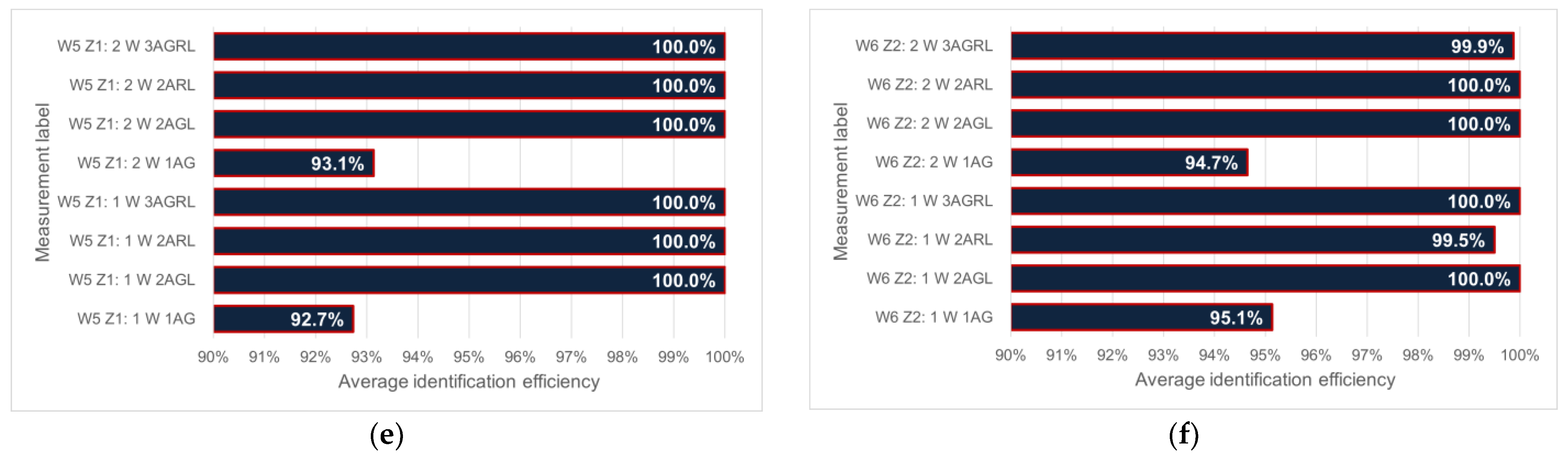
3.2. Dependence of Identification Efficiency on the Number of Objects—Measurement Results
4. Conclusions
Author Contributions
Funding
Institutional Review Board Statement
Informed Consent Statement
Data Availability Statement
Conflicts of Interest
References
- Finkenzeller, K. RFID Handbook—Fundamentals and Applications in Contactless Smart Cards, Radio Frequency Identification and Near-Field Communication, 3rd ed.; Wiley: Hoboken, NJ, USA, 2010. [Google Scholar]
- Dobkin, D.M. The RF in RFID: UHF RFID in Practice, 2nd ed.; Newnes: Oxford, UK, 2012. [Google Scholar]
- Honarvar, M.G.; Latifi, M. Overview of wearable electronics and smart textiles. J. Text. Inst. 2017, 108, 631–652. [Google Scholar] [CrossRef]
- Koncar, V. Introduction to Smart Textiles and Their Applications; Elsevier: Amsterdam, The Netherlands, 2016; ISBN 9780081005835. [Google Scholar]
- Schneegas, S. Smart Textiles Fundamentals, Design, and Interaction; Springer: New York, NY, USA, 2017; ISBN 978-3-319-50123-9. [Google Scholar]
- Moraru, A.; Helerea, E.; Ursachi, C.; Călin, M.D. RFID system with passive RFID tags for textiles. In Proceedings of the 10th International Symposium on Advanced Topics in Electrical Engineering (ATEE), Bucharest, Romania, 23–25 March 2017. [Google Scholar]
- Virkki, J.; Wei, Z.; Liu, A.; Ukkonen, L.; Björninen, T. Wearable passive E-textile UHF RFID tag based on a slotted patch antenna with sewn ground and microchip interconnections. Int. J. Antennas Propag. 2017, 2017, 3476017. [Google Scholar] [CrossRef]
- Moraru, A.; Ursachi, C.; Helerea, E. A New Washable UHF RFID Tag: Design, Fabrication, and Assessment. Sensors 2020, 20, 3451. [Google Scholar] [CrossRef]
- Ukkonen, L.; Sydänheimo, L.; Rahmat-Samii, Y. Sewed textile RFID tag and sensor antennas for on-body use. In Proceedings of the 6th European Conference on Antennas and Propagation, Prague, Czech Republic, 25–30 March 2012. [Google Scholar]
- Luo, C.; Gil, I.; Fernández-García, R. Wearable Textile UHF-RFID Sensors: A Systematic Review. Materials 2020, 13, 3292. [Google Scholar] [CrossRef] [PubMed]
- Corchia, L.; Monti, G.; Tarricone, L. Wearable antennas: Nontextile versus fully textile solutions. IEEE Antennas Propag. Mag. 2019, 61, 71–83. [Google Scholar] [CrossRef]
- Lai, Y.-C.; Chen, S.-Y.; Hailemariam, Z.L.; Lin, C.-C. A Bit-Tracking Knowledge-Based Query Tree for RFID Tag Identification in IoT Systems. Sensors 2022, 22, 3323. [Google Scholar] [CrossRef]
- Arjona, L.; Landaluce, H.; Perallos, A.; Onieva, E. Dynamic Frame Update Policy for UHF RFID Sensor Tag Collisions. Sensors 2020, 20, 2696. [Google Scholar] [CrossRef]
- Filho, I.E.D.B.; Silva, I.; Viegas, C.M.D. An Effective Extension of Anti-Collision Protocol for RFID in the Industrial Internet of Things (IIoT). Sensors 2018, 18, 4426. [Google Scholar] [CrossRef]
- Huang, Z.; Xu, R.; Chu, C.; Li, Z.; Qiu, Y.; Li, J.; Ma, Y.; Wen, G. A Novel Cross Layer Anti-Collision Algorithm for Slotted ALOHA-Based UHF RFID Systems. IEEE Access 2019, 7, 36207–36217. [Google Scholar] [CrossRef]
- Fu, Z.; Deng, F.; Wu, X. Design of a Quaternary Query Tree ALOHA Protocol Based on Optimal Tag Estimation Method. Information 2017, 8, 5. [Google Scholar] [CrossRef]
- Lin, Y.-H.; Liang, C.-K. A Highly Efficient Predetection-Based Anticollision Mechanism for Radio-Frequency Identification. J. Sens. Actuator Netw. 2018, 7, 13. [Google Scholar] [CrossRef]
- Vales-Alonso, J.; Bueno-Delgado, V.; Egea-Lopez, E.; Gonzalez-Castano, F.J.; Alcaraz, J. Multiframe Maximum-Likelihood Tag Estimation for RFID Anticollision Protocols. IEEE Trans. Ind. Inform. 2011, 7, 487–496. [Google Scholar] [CrossRef]
- Alcaraz, J.J.; Vales-Alonso, J.; Egea-Lopez, E.; Garcia-Haro, J.J. A Stochastic Shortest Path Model to Minimize the Reading Time in DFSA-Based RFID Systems. IEEE Commun. Lett. 2013, 17, 341–344. [Google Scholar] [CrossRef]
- Arjona, L.; Landaluce, H.; Perallos, A.; Onieva, E. Timing-Aware RFID Anti-Collision Protocol to Increase the Tag Identification Rate. IEEE Access 2018, 6, 33529–33541. [Google Scholar] [CrossRef]
- Guo, K.; Xie, X.; Qi, H.; Li, K. A High Time-Efficient Missing Tag Detection Scheme for Integrated RFID Systems. Sensors 2022, 22, 4601. [Google Scholar] [CrossRef]
- Espin, J.J.A.; Egea-Lopez, E.; Vales-Alonso, J.; Haro, J.G. Dynamic system model for optimal configuration of mobile RFID systems. Comput. Netw. 2011, 55, 74–83. [Google Scholar]
- Pawłowicz, B.; Trybus, B.; Salach, M.; Jankowski-Mihułowicz, P. Dynamic RFID Identification in Urban Traffic Management Systems. Sensors 2020, 20, 4225. [Google Scholar] [CrossRef]
- Standard International Organization for Standardization/International Electrotechnical Commission. Information Technology—Radio Frequency Identification for Item Management—Part 63: Parameters for Air Interface Communications at 860 MHz to 960 MHz Type C; ISO/IEC: Geneva, Switzerland, 2015; p. 18000-63. [Google Scholar]
- Sabat, W.; Klepacki, D.; Kamuda, K.; Kuryło, K. Analysis of Electromagnetic Field Distribution Generated in a Semi-Anechoic Chamber in Aspect of RF Harvesters Testing. IEEE Access 2021, 9, 92043–92052. [Google Scholar] [CrossRef]
- NXP: SL3S1214 UCODE 7m. Available online: www.nxp.com (accessed on 11 April 2022).
- GS1 EPCglobal. EPC Radio-Frequency Identity Protocols Generation-2 UHF RFID; Specification for RFID Air Interface Protocol for Communications at 860 MHz–960 MHz, Ver. 2.1; EPCglobal: Brussels, Belgium, 2018. [Google Scholar]
- Jankowski-Mihułowicz, P.; Węglarski, M.; Chamera, M.; Pyt, P. Textronic UHF RFID Transponder. Sensors 2021, 21, 1093. [Google Scholar] [CrossRef]
- Pei, J.; Fan, J.; Zheng, R. Protecting Wearable UHF RFID Tags with Electro-Textile Antennas: The Challenge of Machine Washability. IEEE Antennas Propag. Mag. 2021, 63, 43–50. [Google Scholar] [CrossRef]
- Węglarski, M.; Jankowski-Mihułowicz, P. Factors Affecting the Synthesis of Autonomous Sensors with RFID Interface. Sensors 2019, 19, 4392. [Google Scholar] [CrossRef] [PubMed]
- Gupta, A.; Asad, A.; Meena, L.; Anand, R. IoT and RFID-based Smart Card System Integrated with Health Care, Electricity, QR and Banking Sectors. In Artificial Intelligence on Medical Data, Proceedings of International Symposium, ISCMM 2021, Sikkim, India, 11–12, November 2021; Gupta, M., Ghatak, S., Gupta, A., Mukherjee, A.L., Eds.; Springer Nature: Singapore, 2022. [Google Scholar]
- Gupta, A.; Srivastava, A.; Anand, R.; Chawla, P. Smart Vehicle Parking Monitoring System Using RFID. Int. J. Innov. Technol. Explor. Eng. 2019, 8, 225–229. [Google Scholar]


| BLF Frequency Range, kHz | DR Value |
|---|---|
| 40–95 | 8 |
| 95–465 | 8 or 64/3 |
| 465–640 | 64/3 |
| Encoding Type | TPreTR | |
|---|---|---|
| FM0 | ||
| Miller | ||
| Transponder Response | Response Time |
|---|---|
| RN16 | |
| PC + EPC + CRC16 |
| Assumed Values | Requirements of the Standard | |
|---|---|---|
| T1 | ||
| T2 | ||
| T3 | ||
| T4 |
| RWD Command | The Duration of the Command |
|---|---|
| Type of Time Slot | The Duration of the Time Slot |
|---|---|
| Identification | |
| Empty slot | |
| Collision | |
| Incorrect identification |
Disclaimer/Publisher’s Note: The statements, opinions and data contained in all publications are solely those of the individual author(s) and contributor(s) and not of MDPI and/or the editor(s). MDPI and/or the editor(s) disclaim responsibility for any injury to people or property resulting from any ideas, methods, instructions or products referred to in the content. |
© 2023 by the authors. Licensee MDPI, Basel, Switzerland. This article is an open access article distributed under the terms and conditions of the Creative Commons Attribution (CC BY) license (https://creativecommons.org/licenses/by/4.0/).
Share and Cite
Pawłowicz, B.; Kamuda, K.; Skoczylas, M.; Jankowski-Mihułowicz, P.; Węglarski, M.; Laskowski, G. Identification Efficiency in Dynamic UHF RFID Anticollision Systems with Textile Electronic Tags. Energies 2023, 16, 2626. https://doi.org/10.3390/en16062626
Pawłowicz B, Kamuda K, Skoczylas M, Jankowski-Mihułowicz P, Węglarski M, Laskowski G. Identification Efficiency in Dynamic UHF RFID Anticollision Systems with Textile Electronic Tags. Energies. 2023; 16(6):2626. https://doi.org/10.3390/en16062626
Chicago/Turabian StylePawłowicz, Bartosz, Kazimierz Kamuda, Mariusz Skoczylas, Piotr Jankowski-Mihułowicz, Mariusz Węglarski, and Grzegorz Laskowski. 2023. "Identification Efficiency in Dynamic UHF RFID Anticollision Systems with Textile Electronic Tags" Energies 16, no. 6: 2626. https://doi.org/10.3390/en16062626
APA StylePawłowicz, B., Kamuda, K., Skoczylas, M., Jankowski-Mihułowicz, P., Węglarski, M., & Laskowski, G. (2023). Identification Efficiency in Dynamic UHF RFID Anticollision Systems with Textile Electronic Tags. Energies, 16(6), 2626. https://doi.org/10.3390/en16062626