Study of Electromagnetic Characteristics of Brushless Reverse Claw-Pole Electrically Excited Generators for Automobiles

Abstract

A new type of brushless reverse claw-pole electrically excited generator is proposed for the problems of the low sine degree of the induced electromotive force waveform and the high harmonic content of the output voltage of the conventional electrically excited claw-pole generator. The design uses the equivalent magnetic network method to establish the equivalent magnetic circuit model of the motor and determines the equation for calculating the magnetoresistance of the isosceles trapezoidal variable section claw-pole structure. It derives the mathematical model of the no-load induced electric potential of the generator and completes to optimize the motor parameters with the no-load induced electric potential as the target. This study shows that the brushless reverse claw-pole electrically excited generator has the advantages of uniform magnetic field distribution, high harmonic fundamental amplitude of induced electromotive force and low harmonic content. It can better meet the application requirements compared with the conventional electrically excited claw-pole generator.

1. Introduction

Electrically excited claw-pole generators have been widely used in automobiles because of their simple manufacture, low cost and good working stability. However, with the advancement of automotive technology and the increasing number of electrical equipment in automobiles, the problems of low efficiency, low power density and high harmonic content of voltage of traditional claw-pole generators have become more and more prominent [1,2]. These electric devices have gradually failed to meet the usage requirements. To improve the performance of electrically excited claw-pole generators, a large number of scholars have proposed different solutions.

There are three main common solutions. The first one is to change the excitation method and use permanent magnets instead of electrically excited windings [3]. This solution can effectively improve the air-gap magnetic density, but once the size and arrangement of permanent magnets are determined, it is difficult to adjust the permanent magnetic field [4,5].

The second is to place a ring-shaped structure of permanent magnets between the jaw yokes of the electrically excited jaw-pole generator, and the excitation winding is set on the rotor jaw-pole yoke, forming a tandem hybrid excitation structure [6,7]. This solution can effectively reduce the inter-pole leakage flux. However, since the electrically excited magnetic potential and the permanent magnet potential are in series, the flux generated by the electrically excited winding has to pass directly through the permanent magnet. Furthermore, in order to operate with mixed excitation, the excitation winding must be injected with a large enough current, resulting in a large added copper consumption. At the same time, the permanent magnet may be demagnetized permanently if the excitation winding is connected with a large current [8,9,10].

The third option is to use two rotors, an electrically excited rotor and permanent magnet rotor, coaxially parallel to each other to share the same stator parallel hybrid excitation structure [11,12,13]. This solution can meet the advantages of both the electrically excited claw-pole motor with good performance and permanent magnet motor with a high power density. However, the coaxial parallel arrangement requires a long axial space, which increases the axial length and volume of the motor. Moreover, there are both radial and axial three-dimensional magnetic circuits in this structure, and these increase the complexity of the motor structure and decrease the power density [14,15].

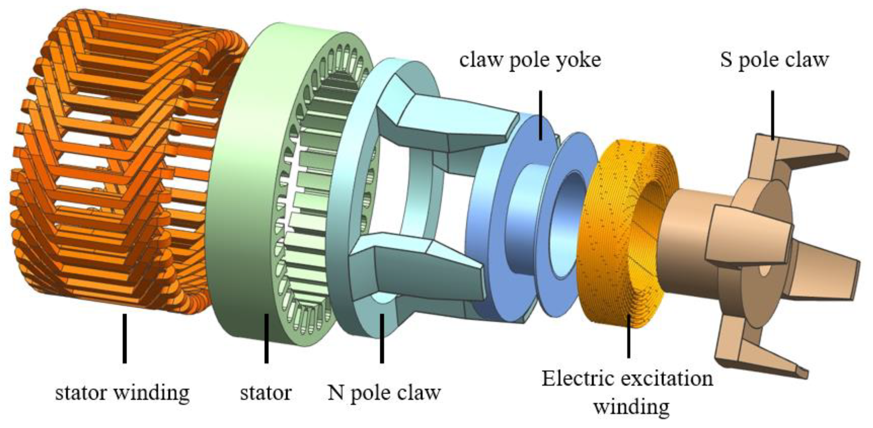
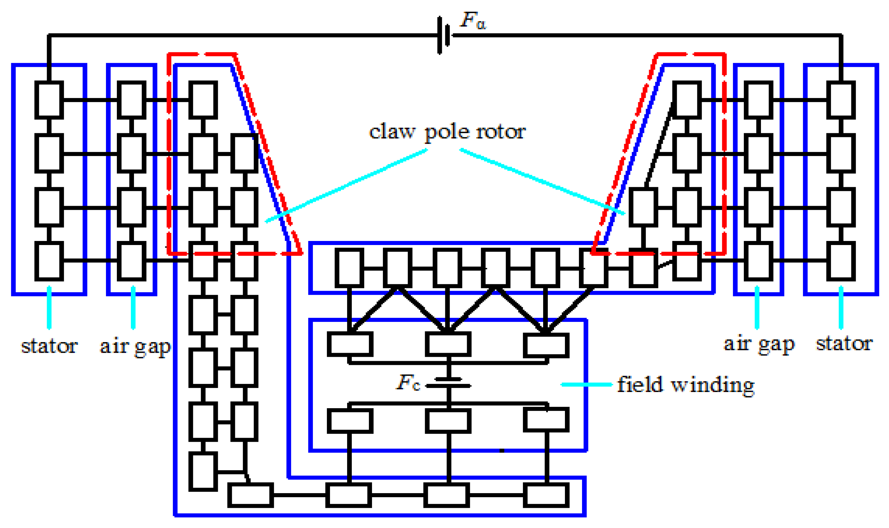
To keep the advantages of simple magnetic field adjustment of the electrically excited claw motor, while strengthening the air-gap magnetic density and increasing the power density, a reverse brushless claw pole is proposed in this paper. The electrically excited rotor extends the rotor N-pole magnetic conductor in a flared shape to form a larger toroidal magnet conductor and shrinks the S-pole magnet conductor in a bottleneck shape to form a smaller toroidal magnet conductor. It then places the excitation winding and toroidal magnet-conducting bridge between the two toroidal magnet conductors to form a reverse claw pole, as shown in Figure 1.

2. Magnetic Circuit Analysis

2.1. Equivalent Magnetic Network Model

The principle of the equivalent magnetic network method is to divide the generator into a number of units with uniform flux distribution and to link each unit according to its actual position in the generator, finally forming a magnetic network [16]. According to the flux distribution in the claw-pole generator, the generator is divided into stator, rotor claw pole, yoke, air gap and so on. For the convenience of expression, the equivalent magnetic network model of a pair of poles of the inverted claw-pole generator in one radial section is given as shown in Figure 2.

The main flux path of the inverted claw-pole generator is simple: electrically excited winding N pole, claw-pole yoke, N-pole flange, N-pole claw-pole support, N-pole claw pole, main air gap, stator core, main air gap, S-pole claw pole, S-pole claw-pole support, S-pole flange, claw-pole yoke and electrically excited winding S pole. Since it is difficult to form a leakage magnetic circuit in the reverse jaw, leakage flux may exist only between the adjacent jaw pole support, adjacent jaw pole and stator teeth.

Based on the equivalent magnetic network model shown in Figure 2, an equivalent magnetic circuit diagram can be created, as shown in Figure 3.

In the Figure 3, $F_c$ is the magnetomotive force of the electrically excited winding; $F_d$ is the stator winding magnetomotive force; ${\Phi }_c$ is the main magnetic flux through the electrically excited winding; ${\Phi }_{\mathit{cf}}$ is the main magnetic flux through the winding yoke; ${\Phi }_{\mathit{cs}}$ is the main magnetic flux through the stator teeth; ${\Phi }_{\mathit{lq}}$ is the leakage flux through the support area of the claw pole; ${\Phi }_{\mathit{lp}}$ is the leakage flux between the poles of the claw pole; ${\Phi }_{\mathit{lg}}$ is the stator tooth leakage flux; $G_c$ is the magnetic permeability of the electrically excited winding; $G_{\mathit{cy}}$ is the magnetic conductivity of the magnetic yoke; $G_{\mathit{cgf}1}$ is the air-gap magnetic conduction between the rear pole yoke and the yoke bracket; $G_{\mathit{cd}}$ is the magnetic conductivity of the yoke bracket; $G_{\mathit{cgf}2}$ is the air-gap magnetic conduction between the anterior yoke and the yoke bracket; $G_{\mathit{cfn}}$ is the air-gap magnetic conduction between the rear pole yoke and the yoke bracket; $G_{\mathit{cd}}$ is the magnetic conductivity of the yoke bracket; $G_{\mathit{cgf}2}$ is the air-gap magnetic conduction between the anterior yoke and the yoke bracket; $G_{\mathit{cfn}}$ is the N-pole flange magnetic conduction; $G_{\mathit{cqn}}$ is the magnetic conductivity of the N-pole claw-pole support; $G_{\mathit{cpn}}$ is the N-pole claw-pole magnetic conductivity; $G_{\mathit{cg}}$ is the main air-gap magnetic conductivity; $G_{\mathit{st}}$ is the magnetic conductivity of the stator teeth; $G_{\mathit{sy}}$ is the magnetic conductivity of the stator yoke; $G_{\mathit{cfs}}$ is the S-pole flange magnetic conductivity; $G_{\mathit{cqs}}$ is the magnetic conductivity of the S-pole claw-pole support; and $G_{\mathit{cps}}$ is the S-pole claw-pole magnetic conductivity.

According to the magnetic circuit shown in Figure 2, we can obtain the following:

$$\left\{\begin{array}{l}{\Phi }_c{=\Phi }_{\mathit{lc}}{+\Phi }_{\mathit{cf}}\\ {\Phi }_{\mathit{cf}}{=\Phi }_{\mathit{lq}}{+\Phi }_{\mathit{lp}}{+\Phi }_{\mathit{lg}}{+\Phi }_{\mathit{cs}}\\ F_c{=\Phi }_{\mathit{cf}}\left(\frac{2}{G_{\mathit{cy}}}+\frac{1}{G_{\mathit{cgf}1}}+\frac{1}{G_{\mathit{cd}}}+\frac{1}{G_{\mathit{cgf}2}}+\frac{1}{G_{\mathit{cfn}}}+\frac{1}{G_{\mathit{cqn}}}+\frac{1}{G_{\mathit{cqs}}}+\frac{1}{G_{\mathit{cfs}}}\right){+\Phi }_{\mathit{lq}}\frac{1}{G_{\mathit{lq}}}{+\Phi }_c\frac{1}{G_c}\\ {\Phi }_{\mathit{lq}}\frac{1}{G_{\mathit{lq}}}=\left({\Phi }_{\mathit{cf}}-{\Phi }_{\mathit{lq}}\right)\left(\frac{1}{G_{\mathit{cpn}}}+\frac{1}{G_{\mathit{cps}}}\right){+\Phi }_{\mathit{lp}}\frac{1}{G_{\mathit{lp}}}\\ {\Phi }_{\mathit{lp}}\frac{1}{G_{\mathit{lp}}}=\left({\Phi }_{\mathit{cf}}-{\Phi }_{\mathit{lq}}-{\Phi }_{\mathit{lp}}\right)\frac{2}{G_{\mathit{cg}}}+{\Phi }_{\mathit{lg}}\frac{1}{G_{\mathit{lg}}}\\ {\Phi }_{\mathit{lg}}\frac{1}{G_{\mathit{lg}}}{=\Phi }_{\mathit{cs}}\left(\frac{2}{G_{\mathit{st}}}+\frac{1}{G_{\mathit{sy}}}\right){+F}_d\end{array}\right.$$

(1)

By using Formula (1), we can obtain the main magnetic flux through the stator tooth:

$${\Phi }_{\mathit{cs}}=\frac{\begin{array}{c}{F}_c-m\left(\frac{2}{G_{\mathit{cy}}}+\frac{1}{G_{\mathit{cgf}1}}+\frac{1}{G_{\mathit{cd}}}+\frac{1}{G_{\mathit{cgf}2}}+\frac{1}{G_{\mathit{cfn}}}+\frac{1}{G_{\mathit{cqn}}}+\frac{1}{G_{\mathit{cqs}}}+\frac{1}{G_{\mathit{cfs}}}+\frac{1}{G_{\mathit{cpn}}}+\frac{1}{G_{\mathit{cps}}}+\frac{2}{G_{\mathit{cg}}}\right)\\ -F_d+F_d{G}_{\mathit{lg}}{G}_{\mathit{lp}}\frac{2}{G_{\mathit{cg}}}\left[\left(\frac{2}{G_{\mathit{cg}}}+\frac{1}{G_{\mathit{lg}}}\right)\left(\frac{2G_{\mathit{lq}}}{G_{\mathit{cg}}}+\frac{G_{\mathit{lq}}}{G_{\mathit{lg}}}+1\right)+1\right]\end{array}}{\left(\frac{2}{G_{\mathit{st}}}+\frac{1}{G_{\mathit{sy}}}\right)+nk-p}$$

(2)

The coefficients m, n, and p are as follows:

$$\begin{array}{ll}m=& F_d{G}_{\mathit{lg}}+F_d{G}_{\mathit{lg}}{G}_{\mathit{lp}}\left(\frac{2}{G_{\mathit{cg}}}+\frac{1}{G_{\mathit{lg}}}\right)+F_d{G}_{\mathit{lg}}{G}_{\mathit{lp}}{G}_{\mathit{lq}}\left(\frac{2}{G_{\mathit{cg}}}+\frac{1}{G_{\mathit{lg}}}\right)\left(\frac{1}{G_{\mathit{cpn}}}+\frac{1}{G_{\mathit{cps}}}\right)\\ & +F_d{G}_{\mathit{lg}}{G}_{\mathit{lq}}\left(\frac{1}{G_{\mathit{cpn}}}+\frac{1}{G_{\mathit{cps}}}\right)+F_d{G}_{\mathit{lg}}{G}_{\mathit{lq}}\left(\frac{2}{G_{\mathit{cg}}}+\frac{1}{G_{\mathit{lg}}}\right)\end{array}$$

(3)

$$\begin{array}{ll}n=G_{\mathit{lg}}\left(\frac{2}{G_{\mathit{st}}}+\frac{1}{G_{\mathit{sy}}}\right)& +G_{\mathit{lp}}{G}_{\mathit{lg}}\left(\frac{2}{G_{\mathit{st}}}+\frac{1}{G_{\mathit{sy}}}\right)\left(\frac{2}{G_{\mathit{cg}}}+\frac{1}{G_{\mathit{lg}}}\right)+\frac{2G_{\mathit{lp}}{G}_{\mathit{lq}}}{G_{\mathit{cg}}}\left(\frac{1}{G_{\mathit{cpn}}}+\frac{1}{G_{\mathit{cps}}}\right)\\ & +G_{\mathit{lp}}{G}_{\mathit{lq}}{G}_{\mathit{lg}}\left(\frac{2}{G_{\mathit{st}}}+\frac{1}{G_{\mathit{sy}}}\right)\left(\frac{2}{G_{\mathit{cg}}}+\frac{1}{G_{\mathit{lg}}}\right)\left(\frac{1}{G_{\mathit{cpn}}}+\frac{1}{G_{\mathit{cps}}}\right)+G_{\mathit{lg}}{G}_{\mathit{lq}}(\frac{2}{G_{\mathit{st}}}\\ & +\frac{1}{G_{\mathit{sy}}})\left(\frac{1}{G_{\mathit{cpn}}}+\frac{1}{G_{\mathit{cps}}}\right)+G_{\mathit{lq}}\left(\frac{1}{G_{\mathit{cpn}}}+\frac{1}{G_{\mathit{cps}}}\right)+G_{\mathit{lq}}{G}_{\mathit{lg}}(\frac{2}{G_{\mathit{st}}}\\ & +\frac{1}{G_{\mathit{sy}}})\left(\frac{2}{G_{\mathit{cg}}}+\frac{1}{G_{\mathit{lg}}}\right)+\frac{2\left(G_{\mathit{lq}}+G_{\mathit{lp}}\right)}{G_{\mathit{cg}}}\end{array}$$

(4)

$$p=G_{\mathit{lg}}{G}_{\mathit{lq}}\frac{2}{G_{\mathit{cg}}}\left(\frac{2}{G_{\mathit{cg}}}+\frac{1}{G_{\mathit{lg}}}\right)\left[\begin{array}{l}\left(\frac{2}{G_{\mathit{cg}}}+\frac{1}{G_{\mathit{lg}}}+\frac{2G_{\mathit{lp}}}{G_{\mathit{cg}}}\right)\left(1+\frac{G_{\mathit{lq}}}{G_{\mathit{cpn}}}+\frac{G_{\mathit{lq}}}{G_{\mathit{cps}}}\right)+\\ +\left(\frac{1}{G_{\mathit{cpn}}}+\frac{1}{G_{\mathit{cps}}}\right)+1+G_{\mathit{lq}}\left(\frac{1}{G_{\mathit{cpn}}}+\frac{1}{G_{\mathit{cps}}}+\frac{2}{G_{\mathit{cg}}}\right)\end{array}\right]$$

(5)

In the formula,

$$\left\{\begin{array}{l}{F}_c=N_{c}I\\ F_d=4.44K_{e}f{N}_{\mathit{st}}{\Phi }_{\mathit{st}}\end{array}\right.$$

(6)

where N_c is excitation coil turns, I is the magnitude of the excitation current, K_e is magnetic flux coefficient, f is the frequency and N_st is number of turns per slot for armature windings.

Then the no-load induced electromotive force is as follows:

$$U=N_d\frac{d{\Phi }_{\mathit{cs}}}{dt}$$

(7)

2.2. Claw-Pole Part Magnetoresistance Calculation

The red dashed part in Figure 2 shows the claw-pole part of the rotor, which has an isosceles trapezoidal variable cross-section structure with different thicknesses tangentially and radially from the claw tip to the claw root. In the tangential direction, the radial cross-section of the claw-pole rotor changes with the angle, θ. Its cross-sectional area varies symmetrically along the central axis of the rotor teeth, so that only half of the rotor teeth need to be considered. When the radial section passes through the central axis of the rotor tooth, the initial value of the defined θ is 0. As the θ increases, the cross-sectional area of rotor tooth decreases and the number of elements it divides decreases. The dividing cell is shown in Figure 4.

In Figure 4, h_i and r_j represent the axial distance and inner diameter of the axial i, tangential j segmentation unit; θ_ij represents the center angle of the segmentation unit; and R is the outer radius of the motor claw-pole rotor. The axial and tangential reluctance of each segmented unit of the claw-pole rotor, shown as R_i and R_j, respectively, are as follows:

$$R_i=\frac{l}{{\mu }_{0}s}=\frac{2h_i}{\mu {\theta }_i{}_j{(r_c^2-r_j^2)}_i}$$

(8)

$$R_j=\frac{l}{{\mu }_{0}s}=\frac{{\theta }_{ij}}{\mu h_i\left(\mathit{ln}{r}_c-\mathit{ln}{r}_j\right)}$$

(9)

where ${\mu }_c$ is claw-pole core relative permeability, and $r_c$ is radius of a segmented unit of the claw-pole tooth.

The tooth axial reluctance, R_cpi, of the claw-pole rotor can be expressed as follows:

$$\begin{array}{l}{R}_{\mathit{cpi}}\\ =\left\{\begin{array}{l}\frac{2L}{\mu {\beta }_1\left(R^2-{(R-b_1)}^2\right)},-\frac{{\beta }_1}{2}<\theta <\frac{{\beta }_1}{2},R-b_1<r<R\\ {{\displaystyle \int }}_{R-b_2}^{R-b_1}\left[{\displaystyle {\displaystyle \sum }_{i=1}^n}\frac{2h_i}{\mu {\beta }_2(\left(R-b_1{)}^2-r^2\right)}\right]dr, -\frac{{\beta }_1}{2}<\theta <\frac{{\beta }_1}{2},R-b_2<r<R-b_1 \\ {{\displaystyle \int }}_{\frac{{\beta }_2-{\beta }_1}{2}}^{\frac{{\beta }_2}{2}}\left[{\displaystyle {\displaystyle \sum }_{i=1}^n}\frac{2h_i}{\mu \theta (R^2-\left(R-b_1{)}^2\right)}\right]d\theta , \frac{{\beta }_1}{2}<\left|\theta \right|<\frac{{\beta }_2}{2},R-b_1<r<R \\ {{\displaystyle \int }}_{R-b_2}^{R-b_1}\left[{{\displaystyle \int }}_{\frac{{\beta }_2-b_1}{2}}^{\frac{{\beta }_2}{2}}\left[{\displaystyle {\displaystyle \sum }_{i=1}^n}\frac{2h_i}{\mu \theta (\left(R-b_1{)}^2-r^2\right)}\right]d\theta \right]dr, \frac{{\beta }_1}{2}<\left|\theta \right|<\frac{{\beta }_2}{2},R-b_2<r<R-b_1 \end{array}\right.\end{array}$$

(10)

where l is the claw-pole axial length, ${\beta }_1$ is the mechanical angle occupied by the claw-pole tip, ${\beta }_2$ is the mechanical angle occupied by the root of the claw pole, $b_1$ is the claw-pole tip thickness and $b_2$ is claw-pole tooth root thickness.

The tooth radial reluctance, R_cpj, of the claw-pole rotor can be expressed as follows:

$$\begin{array}{l}{R}_{\mathit{cpj}}\\ =\left\{\begin{array}{l}\frac{{\beta }_{cj}}{{\mu }_c{l}_{\mathit{cc}}\left[\mathit{ln}R-\mathit{ln}\left(R-h_{\mathit{cj}}\right)\right]},-\frac{{\beta }_{cj}}{2}<\alpha <\frac{{\beta }_{cj}}{2},R-h_{\mathit{cj}}<r<R\\ {{\displaystyle \int }}_{R-h_{\mathit{cg}}}^{R-h_{\mathit{cj}}}\left[{\displaystyle {\displaystyle \sum }_{j=1}^n}\frac{{\beta }_{cj}}{{\mu }_{c}l\left(r\right)\left[\mathit{ln}\left(R-h_{\mathit{cj}}\right)-\mathit{ln}{r}_j\right]}\right]dr, -\frac{{\beta }_{cj}}{2}<\alpha <\frac{{\beta }_{cj}}{2},R-h_{\mathit{cg}}<r<R-h_{\mathit{cj}} \\ {{\displaystyle \int }}_{\frac{{\beta }_{\mathit{cg}}-{\beta }_{\mathit{cj}}}{2}}^{\frac{{\beta }_{\mathit{cg}}}{2}}\left[\frac{{\beta }_{\mathit{cg}}-{\beta }_{\mathit{cj}}}{2{\mu }_{c}l\left(\alpha \right)\left[\mathit{ln}R-\mathit{ln}\left(R-h_{\mathit{cj}}\right)\right]}\right]d\alpha , \frac{{\beta }_{cj}}{2}<\left|\alpha \right|<\frac{{\beta }_{cg}}{2},R-h_{\mathit{cj}}<r<R \\ {{\displaystyle \int }}_{R-h_{\mathit{cg}}}^{R-h_{\mathit{cj}}}\left[{{\displaystyle \int }}_{\frac{{\beta }_{\mathit{cg}}-h_{\mathit{cj}}}{2}}^{\frac{{\beta }_{\mathit{cg}}}{2}}\left[{\displaystyle {\displaystyle \sum }_{j=1}^n}\frac{{\beta }_{\mathit{cg}}-{\beta }_{\mathit{cj}}}{{\mu }_{c}l\left(\alpha ,r\right)\left[\mathit{ln}\left(R-h_{\mathit{cj}}\right)-\mathit{ln}{r}_j\right]}\right]d\alpha \right]dr,\frac{{\beta }_{cj}}{2}<\left|\alpha \right|<\frac{{\beta }_{cg}}{2},R-h_{\mathit{cg}}<r<R-h_{\mathit{cj}} \end{array}\right.\end{array}$$

(11)

The magnetic permeability of the teeth of the claw-pole rotor is as follows:

$$G_{\mathit{cpn}}=G_{\mathit{cps}}=\frac{1}{\sqrt{R_{\mathit{cpi}}^2+R_{\mathit{cpj}}^2}}$$

(12)

To simplify the calculation process, the part of the reluctance that is uniform and has a regular shape does not need to be split to solve, and the remaining part of motor magnetoresistance is not repeated in this article.

3. Finite Element Analysis

Taking a 3-phase, 8-pole, 36-slot reverse claw-pole electrically excited generator (rated power of 2 kW, rated voltage of 72 V and rated speed of 3000 r/min) as an example, a two-dimensional simulation model is established by using Maxwell finite element analysis software to verify the accuracy of the mathematical model.

Table 1. Reverse claw-pole electrically excited generator part of the structural parameters.

Parameter	Numeric Value	Unit
Claw-pole axial length	30	mm
Claw-pole tip width	17	mm
Claw-pole tooth root width	24	mm
Claw-pole tip thickness	3.5	mm
Claw-pole tooth root thickness	10	mm
Claw-pole outer diameter	50.6	mm
Stator outer diameter	68	mm
Stator inner diameter	51.2	mm

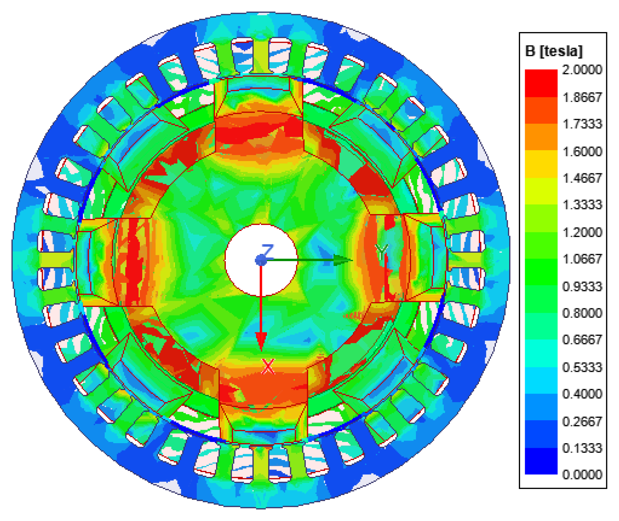
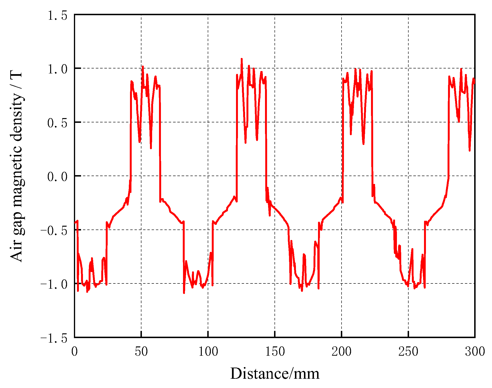
shows some structural parameters of the reverse claw-pole electrically excited generator. Figure 5 shows the magnetic flux density cloud of the reverse claw-pole electrically excited generator. Figure 6 shows the magnetic density distribution of the air gap at the root of the claw pole. The simulation results show that the maximum magnetic density in the air gap is 1.09 T.

It is necessary to show the distribution of the air gap more clearly, so the magnetic flux density cloud map from the outer diameter of the claw pole to the inner diameter of the stator in the axial middle position of the claw pole is shown in Figure 7. Moreover, the magnetic flux density cloud map from the root of the claw to the tip of the claw in the radial middle position of the air gap is shown in Figure 8. From these figures, it can be seen that the flux density at the claw root is larger than that at the claw tip under the same air gap radius. Moreover, at the same distance from the claw root, the smaller the air gap radius is, the largest flux density is.

Figure 9 shows the no-load induced electromotive force waveform of the inverted claw-pole electrically excited generator, and the induced electromotive force waveform is basically sinusoidal with the maximum value of 38.82 V. Taking the Fourier decomposition of the induced electromotive force of phase A, the histogram of the harmonic distribution of the induced electromotive force can be obtained as shown in Figure 10. From Figure 10, it can be seen that the fundamental waveform amplitude is 33.63 V; the amplitude of each harmonic is shown in

Table 2. Optimization constraints of each design variable.

Design Variable	Symbol	Initial Value	Unit	Binding Conditions
Width of claw-pole tooth tip	a1	17	mm	16 ≤ a1 ≤ 18
Width of claw-pole tooth root	a2	24	mm	23 ≤ a2 ≤ 25
Claw-pole tooth tip thickness	b1	3.5	mm	3 ≤ b1 ≤ 4.5
Claw-pole tooth root thickness	b2	10	mm	9.5 ≤ b2 ≤ 12

, and the waveform distortion rate THD calculation for A-phase induced potential is 19.8%.

Changes in some structural parameters of the claw-pole rotor can significantly affect the generator performance and need to be optimized. However, the structural parameters of the claw pole are not independent, and the interconnection between the parameters and the influence of the parameters on the generator performance are complex and variable. According to the sensitivity of each parameter to the induction potential of the generator, the design variables are selected as the claw-pole tip arc coefficient, claw-pole root arc coefficient, claw-pole tooth tip thickness and claw-pole tooth root thickness. The base wave amplitude and sinusoidal distortion rate of the induction potential of the generator are the two optimization objectives. The constraints of each design variable are shown in Table 2.

The optimization objective is to maximize the fundamental of the inductive electric potential and minimize the sinusoidal distortion rate while satisfying the constraints, and the optimization model is shown as follows.

$$\left\{\begin{array}{l}\mathit{max}{U}_A\left(x_1,x_2,...,x_m\right)\\ \mathit{min}THD\left(x_1,x_2,...,x_m\right)\end{array}\right.$$

(13)

where U_A represents the phase-A induced electromotive force fundamental amplitude, and THD represents the induced electromotive force waveform distortion rate.

Due to the special characteristics of the claw-pole rotor structure, a three-dimensional model needs to be established for the finite element simulation calculation, and the calculation volume is large; thus, the Latin super-erection method with an optimized number of 100 sample points is used for sample collection of the design variables. Some of the sampling points are shown in

Table 3. Some sampling points correspond to design variable values.

Serial Number	a1	a2	b1	b2
0	17	24	3.5	10
1	17.1565	24.0115	3.4125	10.1725
2	16.9045	23.9275	3.8925	10.6225
3	17.1475	23.8225	4.3275	11.0725
…	…	…	…	…
96	17.0365	23.9335	3.6375	10.7425
97	16.9645	23.8945	4.4775	11.2225
99	16.9585	23.9815	3.9675	10.6675
100	16.9405	23.8315	4.4175	10.5625

, where sample point 0 is the initial value of the design variables.

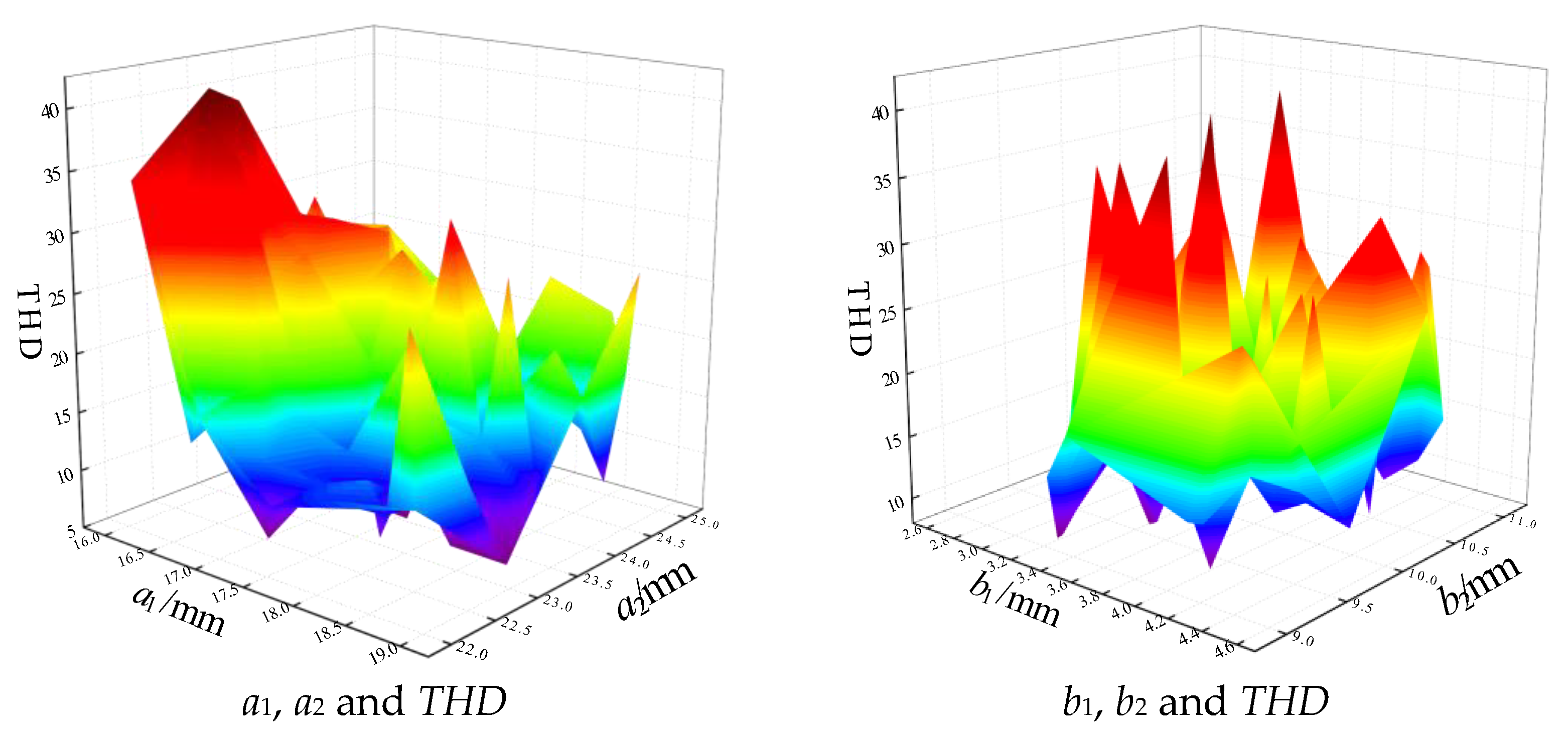
A simulation analysis is performed for 100 sampling points, and a plot of the fitted surface relationship between the design variables and the response values can be obtained. Some of the design variables and response values’ fitted relationship graphs are shown in Figure 11.

As can be seen from Figure 11, a₁, a₂ and the induced electric potential have an approximately single-peak linear relationship. The spatial relationships between the design variables and the response values have multi-peak, multi-valley, non-uniform and non-linear characteristics.

The characteristics of the effect of each design variable on the response value can be obtained from the fitted relationship between the design variables and the response value. It can be expressed by the sensitivity of each design variable to the change in the response value. The sensitivity of each design variable is shown in

Table 4. Sensitivity of the design variable with respect to the response value.

Design Variables	Sensitivity for UA	Sensitivity for THD
a1	0.55476	0.51572
a2	0.33641	0.11612
b1	0.15723	0.05364
b2	0.03547	0.03674

.

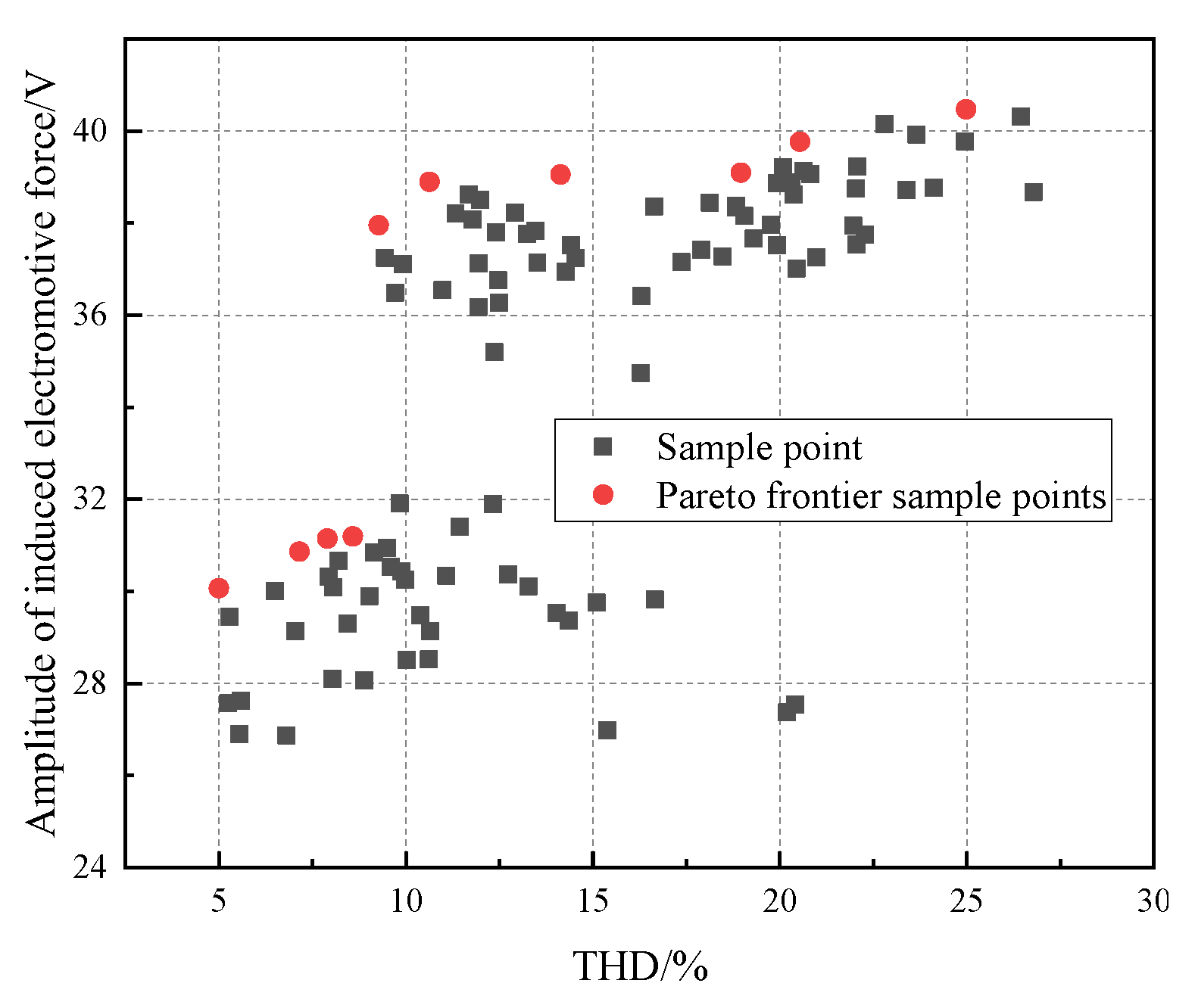
The pareto optimization method is a common method for solving multi-objective optimization problems, especially for two-objective optimal problems [17,18]. By solving the Pareto front, the distribution of the optimal solution set can be reflected intuitively in the two-dimensional space. The full sample points were counted, and their Pareto front distribution is shown in Figure 12.

As can be seen from Figure 12, there are 10 sample points on the Pareto front. These 10 sample points are the valid solutions of this optimization model, respectively, and the specific values of the design variables and optimization objectives at this time are shown in

Table 5. The specific values of design variables and optimization objectives in the effective solution.

Serial Number	a1	a2	b1	b2	THD/%	UA/V
74	17.0485	23.8885	3.0225	10.5025	5.31	30.06
6	17.0665	23.8615	3.9075	10.9675	7.16	30.86
31	16.9645	23.8945	4.4775	11.2225	7.90	31.14
43	17.0815	23.9245	3.0375	11.0875	8.58	31.19
15	17.0365	23.9335	3.6375	10.7425	9.27	37.95
37	16.9825	23.9215	3.9975	10.3675	10.63	38.89
24	17.1805	23.9485	4.0875	11.4025	17.13	39.05
86	16.9585	23.9815	3.9675	10.6675	18.18	39.69
37	17.0935	23.9305	4.4325	11.4625	20.53	39.76
92	16.9405	23.8315	4.4175	10.5625	24.97	40.47

.

To determine the relative optimal solution, K is defined and represents the parameter matching coefficient. The larger the value, the better the corresponding motor output performance, while assigning weights to the two optimization objectives. The expression of this is as follows:

$$\begin{array}{c}K=C_1\frac{U_A\left(x_1,x_2,...,x_m\right)}{U_0}-\frac{C_2}{100}THD\left(x_1,x_2,...,x_m\right)\end{array}$$

(14)

In the formula, K is the performance parameter match factor, which represents the ultimate performance superiority of the motor; C₁ and C₂ are weighting coefficients, where C₁ takes 0.6 and C₂ takes 0.4; and U₀ is the generator induces the electromotive force fundamental amplitude at the initial value of the design variable.

From this equation, the relationship between the two optimization objectives and K among the 10 valid solutions solved by the Pareto front can be obtained. The two optimization objectives are plotted against the matching coefficients, as shown in Figure 13.

As can be seen from Figure 13, sample point No. 37 is the “optimal solution” of the optimization model, at which the fundamental amplitude of the motor induction potential is 38.89V and the waveform distortion rate is 10.63%. The final value is obtained based on the values of the variables and the actual machining process. The optimal solution and the final value of each response variable are shown in

Table 6. Optimal solution and final value of each response variable.

Parameters	Optimal Solution	Final Value
a1	16.9825	17.0
a2	23.9215	23.9
b1	3.9975	4.0
b2	11.4675	11.5

.

4. Experimental Validation

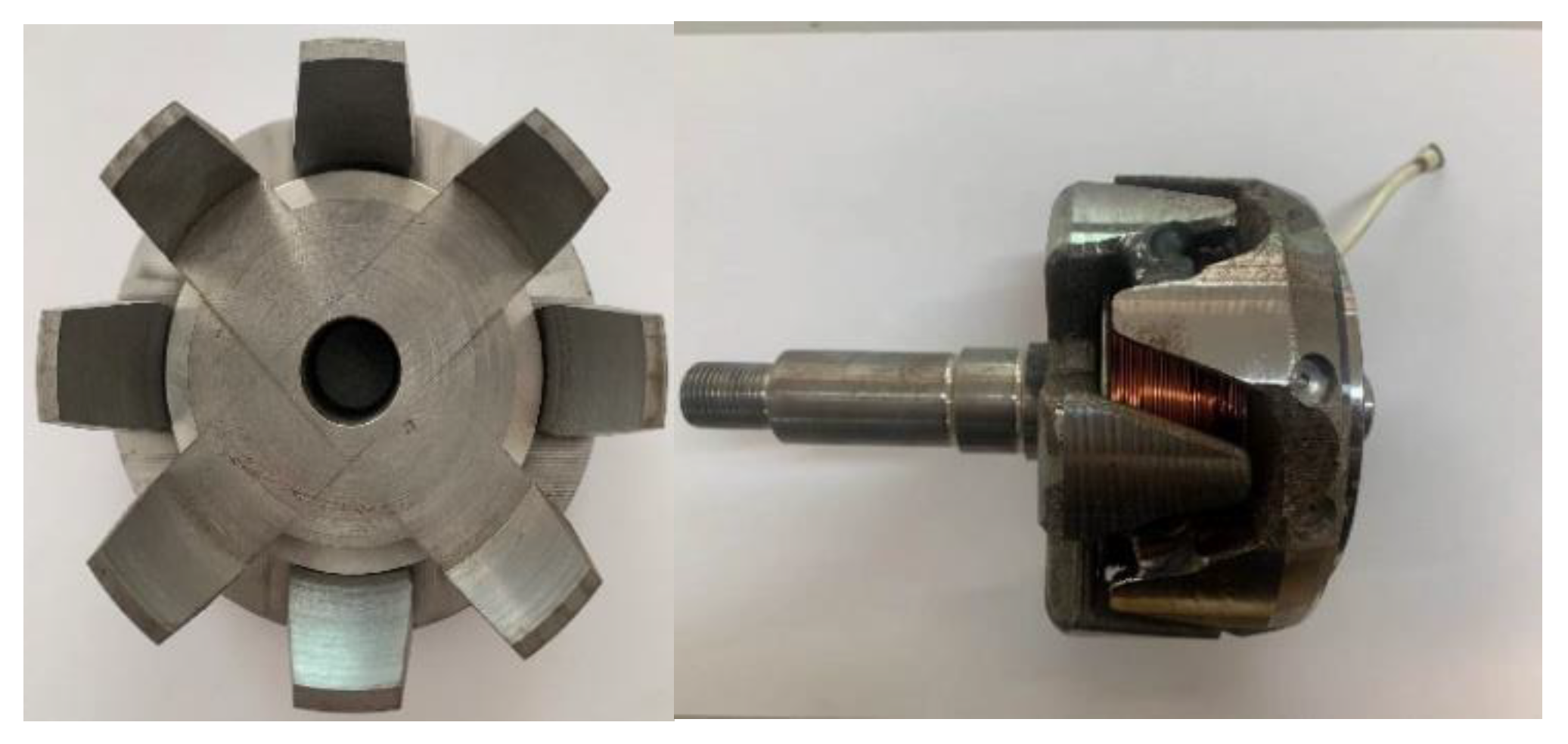
Based on the optimized motor parameters, the prototype is fabricated, and its performance is tested by using the generator test bench. The reverse brushless claw-pole electrically excited prototype and the conventional claw-pole electrically excited generator are shown in Figure 14, and the generator test bench is shown in Figure 15.

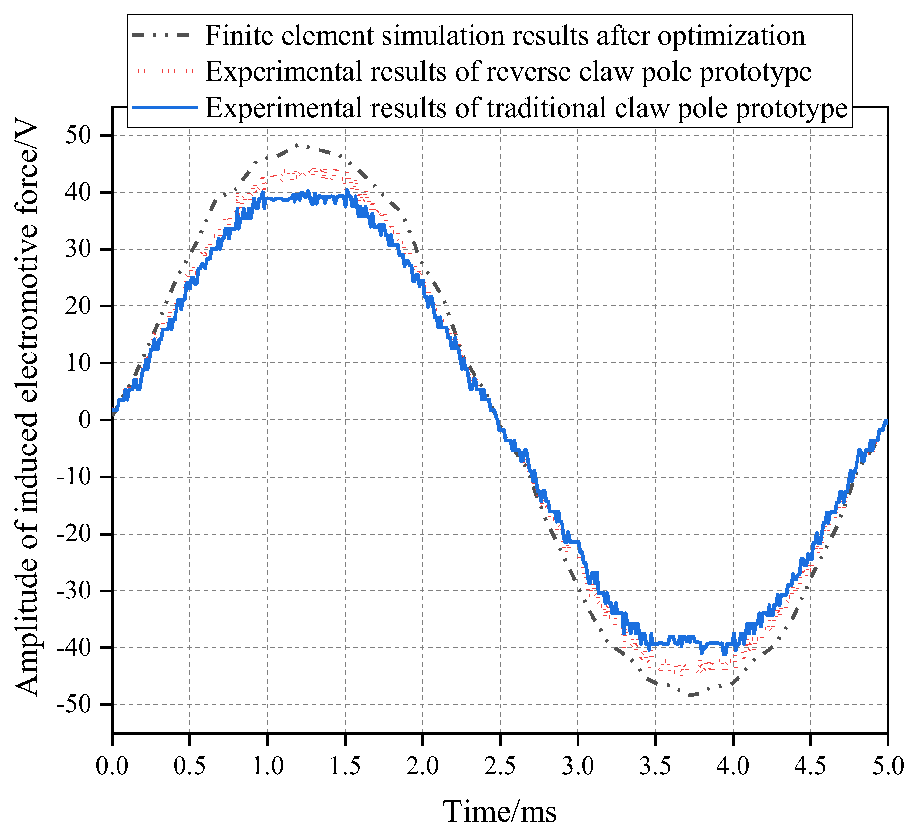
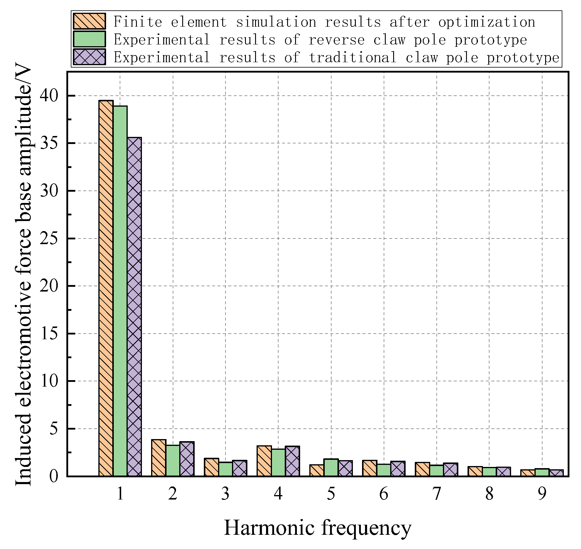
The no-load characteristics of the test prototype were obtained, and the no-load induced electromotive force curve and no-load induced electromotive force harmonic distribution of the generator were compared with the optimized finite element analysis results. The comparison results are shown in Figure 16, Figure 17 and

Table 7. Data comparison of experimental results.

	Amplitude of Fundamental Wave of Induced Electromotive Force/V	THD/%
Finite element simulation results after optimization	38.89	10.63
Experimental results of reverse claw-pole prototype	38.23	13.32
Experimental results of traditional claw-pole prototype	35.37	17.47

.

As can be obtained from Figure 16, Figure 17 and Table 7, the no-load induced electromotive force waveform obtained from the performance test of the reverse claw-pole prototype is basically the same as the simulation result. It can be seen that the value at the peak is slightly lower, and the waveform has good sinuosity. The test results show that the fundamental amplitude of the no-load inductive electromotive force of the reverse claw polar prototype machine is 38.23 V. The error with the simulation result is 1.7%, and the distortion rate of the no-load induction electromotive force is 13.32%. The reason for the error with the test result is that the simulation value is only taken from the first nine harmonics, which is slightly lower than the actual value. Moreover, the test value can be accurately calculated by the generator test bench for all harmonics.

The waveform of no-load induction potential of the conventional claw-pole prototype has the phenomenon of “clipping” at the peak and trough; the base wave amplitude of the no-load induction potential is 35.37 V, and the distortion rate is 18.47%, which are different from the performance of the reverse claw-pole prototype. This is due to the structural limitations of the conventional claw motor-excited generator; in the case of the same rotor diameter, the width of the claw tip is significantly smaller than that of the reverse claw generator. The width of the claw tip of the tests prototype is only 8 mm.

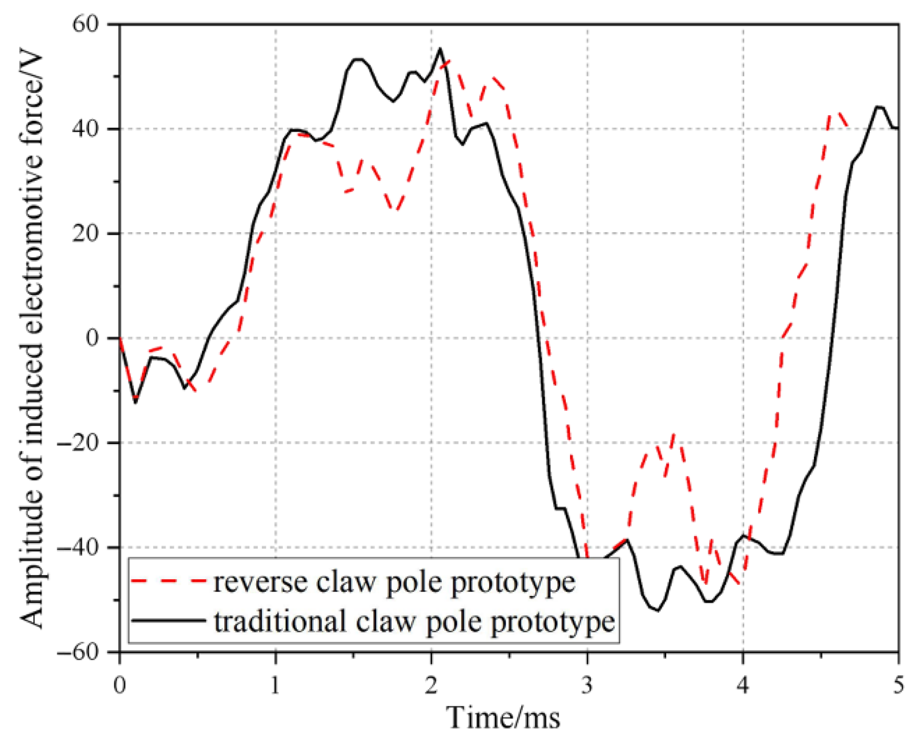
Figure 18 and Figure 19 show the variation curves of the induced electromotive force of the generator at a load of 50 Ω and 100 Ω, respectively. It can be seen from the figure that, with the increase of the load, the induced electromotive force waveform distortion of the traditional claw motor generator is greater. At a 100 Ω load, the induced electromotive force has an obvious depression at the crest and trough of the waveform. At the same time, the maximum induced electromotive force of the reverse claw-pole generator is greater than that of the traditional claw-pole generator.

5. Conclusions

This paper proposes a brushless reverse claw-pole electrically excited generator, which has the advantages of uniform magnetic field distribution, high-power density and low harmonic content of induction electric potential compared with the traditional electrically excited claw-pole generator. The whole machine adopts a brushless structure, eliminating the carbon brush slip ring structure and making it is easy to wear, and the whole machine is highly reliable. The article aims at a high base wave amplitude and low waveform distortion rate of the induction potential at no load, completes the optimization of the machine parameters and determines the optimal claw-pole size. After optimization, the base wave amplitude of the induction potential is 38.89 V, and the waveform distortion rate is 10.63%. The trial prototype and test show that reverse claw-pole electrically excited generator has high sinusoidality, a high fundamental amplitude and a low waveform distortion rate under different loads’ power-generation conditions. Its performance is significantly better than that of traditional claw generators, which can better meet the application requirements.

References

1. Zhang, Z.; Wang, D.; Hua, W. Summary and prospect of structure principle, design and operation control technology of hybrid excitation motor. Proc. CSEE 2020, 40, 7834–7850+8221. [Google Scholar]
2. Wang, Q.; Ni, Y.; Zhang, X.; Li, Z. Load characteristics of hybrid excitation claw pole generator are calculated based on three-dimensional equivalent magnetic network method. J. Electr. Technol. 2006, 21, 96–100. [Google Scholar]
3. Cros, J.; Viarouge, P. New structure of polyphase claw-pole machine. IEEE Trans. Ind. Appl. 2004, 40, 113–120. [Google Scholar] [CrossRef]
4. Hua, B.; Steven, D.; Pekarek, S.D. Analytical derivation ofa coupled-circuited model of a claw-pole alternator with concentrated stator windings. IEEE Trans. Energy Convers. 2002, 17, 32–38. [Google Scholar]
5. Li, B.; Li, X.; Wang, S.; Liu, R.; Wang, Y.; Lin, Z. Analysis and Cogging Torque Minimization of a Novel Flux Reversal Claw Pole Machine with Soft Magnetic Composite Cores. Energies 2022, 15, 1285. [Google Scholar] [CrossRef]
6. Zhao, C. Structure design and characteristics of series magnetic circuit hybrid excitation claw pole generator. Trans. Electr. Technol. 2009, 24, 12. [Google Scholar]
7. Du, W.; Zhao, S.; Zhang, H.; Zhang, M.; Gao, J. A Novel Claw Pole Motor With Soft Magnetic Composites. IEEE Trans. Magn. 2021, 57, 8200904. [Google Scholar] [CrossRef]
8. Kim, J.S.; Kim, D.W.; Kim, Y.J.; Jung, S.Y. Field-Winding Claw-Pole Type Motor Characteristics Analysis Using Additional Ferrite Magnets. J. Magn. 2019, 24, 179–183. [Google Scholar] [CrossRef]
9. Wardach, M. Hybrid Excited Claw Pole Generator with Skewed and Non-skewed Permanent Magnets. Open Phys. 2017, 15, 902–906. [Google Scholar] [CrossRef]
10. Wang, X.; Li, N.; Zhao, X.; Pang, W. Magnetic field design of a claw-pole hybrid excitation belt driven starter/generator. Trans. Electr. Technol. 2020, 35, 4258–4265. [Google Scholar]
11. Cao, Y.; Liu, C.; Yu, J. Mesh-Based 3D MEC Modeling of a Novel Hybrid Claw Pole Generator. Energies 2022, 15, 1692. [Google Scholar] [CrossRef]
12. Geng, H.; Zhang, X.; Zhang, Y.; Hu, W.; Lei, Y.; Xu, X.; Wang, A.; Wang, S.; Shi, L. Development of Brushless Claw Pole Electrical Excitation and Combined Permanent Magnet Hybrid Excitation Generator for Vehicles. Energies 2020, 13, 4723. [Google Scholar] [CrossRef]
13. Fu, X.; Zou, J. Numerical analysis on the magnetic field of hybrid exciting synchronous generator. IEEE Trans. Magn. 2009, 45, 4590–4593. [Google Scholar]
14. Chen, Z.; Wang, B.; Chen, Z.; Yan, Y. Comparison of flux regulation ability of the hybrid excitation doubly salient machines. IEEE Trans. Ind. Electron. 2014, 61, 3155–3166. [Google Scholar] [CrossRef]
15. Sun, L.; Zhang, Z.; Yu, L.; Gu, X. Development and analysis of a new hybrid excitation brushless de generator with flux modulationeffect. ΙΕΕΕ Trans. Ind. Electron. 2019, 66, 4189–4198. [Google Scholar] [CrossRef]
16. Yeo, H.K.; Lim, D.K.; Jung, H.K. Magnetic equivalent circuit model considering the overhang structure of an interior permanent-magnet machine. IEEE Trans. Magn. 2019, 55, 1–4. [Google Scholar] [CrossRef]
17. Wu, G.; Que, L.; Ju, C. A two-objective and two-stage grid voltage optimization method based on Pareto front. Syst. Sci. Math. 2021, 41, 3207–3217. [Google Scholar]
18. Hu, X.B.; Gu, S.H.; Zhang, C.; Zhang, G.P.; Zhang, M.K.; Leeson, M.S. Finding all Pareto optimal paths by simulating ripple relay race in multi-objective networks. Swarm Evol. Comput. 2021, 64, 100908. [Google Scholar] [CrossRef]
Figure 1. Structure diagram of reverse brushless claw-pole generator.
Energies 16 02573 g001
Figure 2. Equivalent magnetic network model.
Energies 16 02573 g002
Figure 3. Equivalent magnetic network diagram.
Energies 16 02573 g003
Figure 4. A tessellation unit.
Energies 16 02573 g004
Figure 5. Flux density cloud of reverse claw-pole electrically excited generator.
Energies 16 02573 g005
Figure 6. Magnetic density distribution of air gap at the root of the claw pole.
Energies 16 02573 g006
Figure 7. Flux density cloud at the middle of the claw pole.
Energies 16 02573 g007
Figure 8. Cloud map of magnetic flux density at the middle of the air gap.
Energies 16 02573 g008
Figure 9. Three-phase no-load induction electromotive force waveform 3 Structure optimization.
Energies 16 02573 g009
Figure 10. Histogram of the harmonic distribution of the induced electric potential.
Energies 16 02573 g010
Figure 11. Part of the design variable fits the response value.
Energies 16 02573 g011aEnergies 16 02573 g011b
Figure 12. Pareto frontier distribution map.
Energies 16 02573 g012
Figure 13. The relationship between the two optimization objectives and the matching coefficient.
Energies 16 02573 g013
Figure 14. Reverse brushless claw-pole electrically excited prototype and conventional claw-pole electrically excited generator.
Energies 16 02573 g014
Figure 15. Generator test bench.
Energies 16 02573 g015
Figure 16. No-load induced electromotive force curve change.
Energies 16 02573 g016
Figure 17. No-load induced electromotive force harmonic distribution.
Energies 16 02573 g017
Figure 18. Curve change diagram of induced electromotive force under 50 Ω load.
Energies 16 02573 g018
Figure 19. Curve change diagram of induced electromotive force under 100 Ω load.
Energies 16 02573 g019