A Review of Physics-Informed Machine Learning in Fluid Mechanics

Abstract

Physics-informed machine-learning (PIML) enables the integration of domain knowledge with machine learning (ML) algorithms, which results in higher data efficiency and more stable predictions. This provides opportunities for augmenting—and even replacing—high-fidelity numerical simulations of complex turbulent flows, which are often expensive due to the requirement of high temporal and spatial resolution. In this review, we (i) provide an introduction and historical perspective of ML methods, in particular neural networks (NN), (ii) examine existing PIML applications to fluid mechanics problems, especially in complex high Reynolds number flows, (iii) demonstrate the utility of PIML techniques through a case study, and (iv) discuss the challenges and opportunities of developing PIML for fluid mechanics.

1. Introduction

1.1. Background and Motivation

In the last few decades, computational fluid dynamics (CFD) of compressible and incompressible fluid flows has progressed significantly through finite difference, finite volume, finite elements and spectral methods. With the increasing availability of high-performance computational resources, we can now simulate complex turbulent flows at increasingly higher spatial and temporal resolutions. Despite this progress, several challenges still persist for conventional numerical and analytic approaches. For example, solving inverse problems (e.g., for unknown boundary conditions or experimental parameters) is still prohibitively expensive. More importantly, numerical approaches typically simulate configurations under idealized conditions that do not account for realistic processes such as missing or noisy boundary conditions [1]. Moreover, direct numerical simulations (DNS) of many practical turbulent systems are still unfeasible due to the computational complexity of resolving all spatial scales in multi-physical processes. This is especially true for complex flows involving phase transitions or chemical reactions, which may require solving conservation equations for hundreds of species, introducing additional complexity challenges that arise from dimensionality and stiffness.

Machine learning (ML) and data-driven techniques have been increasingly popular in scientific and engineering fields, offering a paradigm shift that can help address these challenges. Recently, with improved hardware, such as graphic processing units (GPUs) and tensor processing units (TPUs), data storage technologies, and access to a plethora of methods through open-source libraries, ML offers new opportunities for investigating modeling and predicting fluid flows. ML can be employed to supplement incomplete domain-specific knowledge in conventional experimental or numerical configuration by (i) exploring large design spaces, (ii) identifying hidden patterns, features or multi-dimensional correlations, and (iii) managing ill-posed problems. As such, ML has become a popular tool for studying fluid flows, especially when combined with the existing domain knowledge and intellectual traditions that arise from the study of physical systems. To this end, this paper aims to review and discuss the intersection of existing physical knowledge with new methods offered by ML toward solving various problems tied to fluid flows.

1.2. Fundamentals and History

Here, we provide a summary of ML fundamentals and a historical perspective. ML can be categorized into supervised, unsupervised, and semi-supervised learning [2]. Supervised learning combines a collection of methods that learn input–output relationships from labeled data [2] (see Figure 1). This is opposed to unsupervised learning, which extracts from unlabeled data, as well as semi-supervised learning, which contains attributes of both supervised and unsupervised learning. Typical applications of supervised learning include classification and regression problems.

Among the most popular algorithms in supervised learning is the neural network (NN), which is also the centerpiece of many deep learning techniques. Given the overwhelming focus across the numerous fields on NNs and deep learning techniques, this review will focus largely on physics-informed supervised and deep learning techniques. In its most basic form, NNs are multi-layer perceptrons (MLPs) consisting of multiple layers, and they generate predictions by forward propagating the outputs of each layer to the next layer. For example, a one-layer MLP makes a prediction $\widehat{y}$ by first evaluating a linear function z from inputs X, weights W, and biases b:

$$\widehat{y}=\sigma \left(z\right)\mathrm{with}z=WX+b.$$

(1)

Nonlinearity is then introduced to z through an activation function, which takes the form of sigmoid, tanh, ReLU, and other nonlinear functions [3]. The weights and biases determine the output of the NN, and they are determined through training, which involves optimizing a loss function through a gradient descent [4] operation.

The key idea behind NNs took form in the 1980s, with the introduction of backpropagation [5]—which leverages chain ruling to significantly reduce the computational costs of training deep learning models by allowing for low-cost evaluations of gradients. Similarly, convolutional neural networks (CNNs)—a commonly used model architecture for application to spatial problems (as encountered in flow physics)—were introduced in the late 1990s [6]. While the concepts behind NNs are not particularly new, the increasing interest in deep learning can be linked to two applications. Firstly, seminal work by Mnih et al. [7,8] in the mid-2010s on deep reinforcement learning (RL) demonstrated the utility and wide-ranging applicability of deep learning algorithms in solving numerous challenging problems. Secondly, a deep learning model with 152 layers was demonstrated by He et al. [9] to outperform human performance in the ImageNet [10] image recognition challenge. This work demonstrated that the combination of deep multi-layer architectures can be combined with powerful GPUs and massive datasets to generate highly accurate predictions.

With the increasing interest in ML methods, data-driven techniques have been applied extensively to a wide range of fluid mechanics and turbulence problems. For example, early works [11,12] focused on examining the feasibility of replacing conventional algebraic turbulence models with ML models. While vanilla (canonical or baseline) ML models possess the necessary expressiveness to model nonlinear turbulent behavior, these studies identified the difficulty in accessing sufficient data as a major bottleneck for ML models to generalize well outside of the training data. As such, many vanilla ML models, which rely solely on the abundance of data, are currently not suited for many tasks in fluid mechanics problems. Hence, the research community has developed interest in an alternate paradigm, which combines existing domain knowledge with ML techniques, which is known as physics-informed ML (PIML).

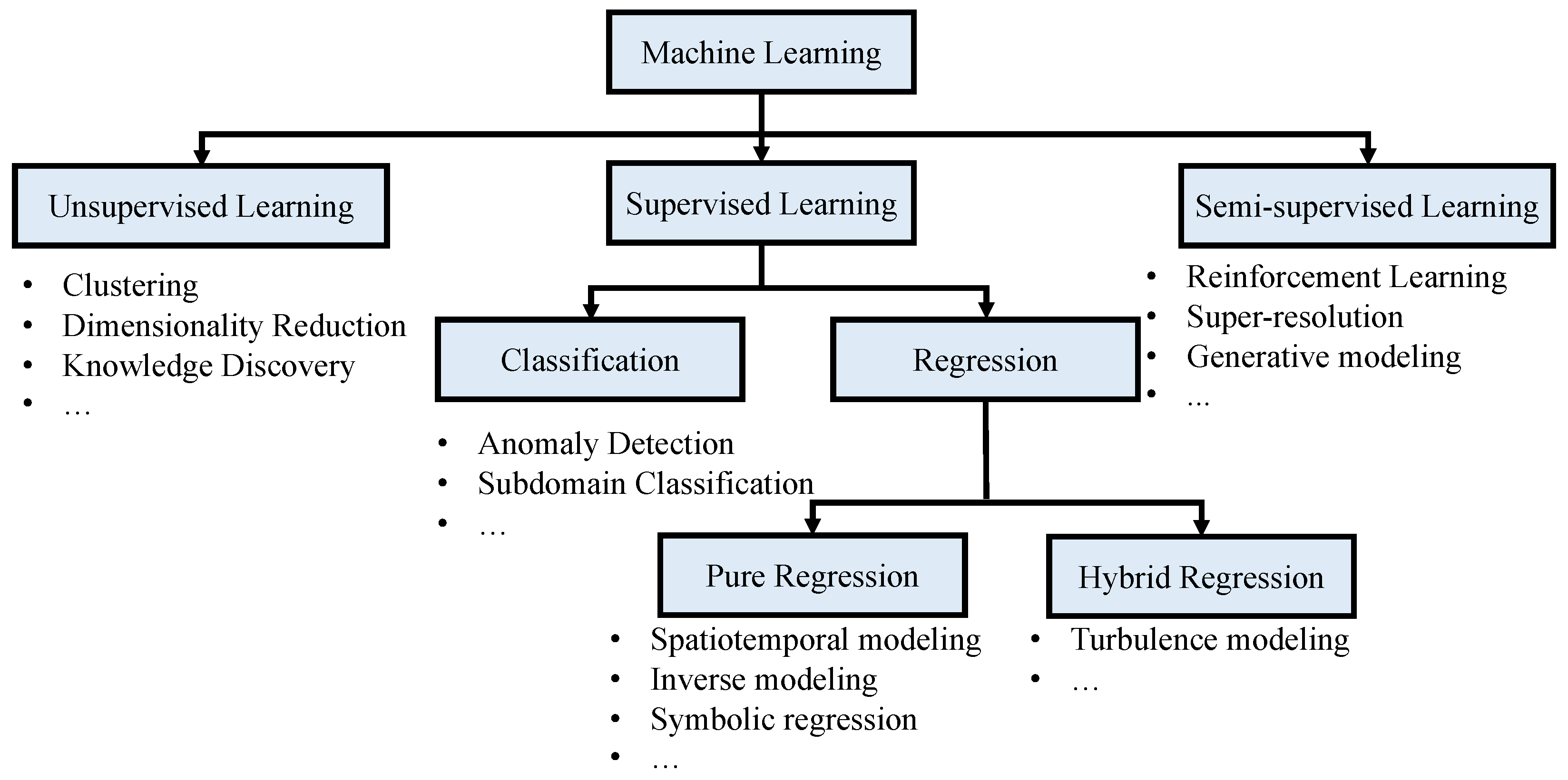
1.3. Applications of ML in Fluid Mechanics

In this section, we categorize and provide examples of ML applications within the study of fluid mechanics. As seen in Figure 1, unsupervised algorithms such as principal component analysis [13] and the k-means [14] algorithm are typically used to process unlabeled data through dimensionality reduction and clustering, respectively. Semi-supervised learning techniques involving RL and generative ML have been applied toward controlling flows [15] and automating turbulence modeling [16]. However, with the exception of super-resolution [17,18] (which involves feeding low-resolution flow field data into generative ML to predict a corresponding upsampled high-resolution flow field), studies involving these techniques have not been investigated as extensively as supervised learning algorithms, which can be broadly categorized into classification and regression problems. Studies employing classification methods are usually limited to problems which require choosing and blending from a set of predefined models within a simulation domain [19,20] as well as detecting faults and anomalous events [21].

When applied to fluid mechanics, regression can be categorized into pure and hybrid approaches, which seek to treat a modeling problem either entirely or partially, respectively. The most popular application of pure regression is the prediction of spatiotemporal dynamics in flow configurations, while inverse modeling [22] and symbolic regression [23,24] enable deducing unknown parameters and formulate algebraic models, respectively. The physics-informed neural network (PINN) [25] has received wide attention for the purposes of pure regression. It leverages well-posed PDE information to make data-driven predictions, even in data-sparse regimes. The utility of PINNs, along with its numerous variants, has been investigated in numerous studies [22,26,27,28,29,30,31,32,33,34,35], on both spatiotemporal and inverse modeling. Other PIML methods for spatiotemporal modeling include the PDE-preserving NN (PPNN) [36], physics-informed convolution recurrent network (PhyCRNet) [37], and several others [38,39,40,41,42,43,44]. Some of these methods will be discussed later in Section 2.

The most popular application of hybrid regression is turbulence closure modeling [45]. Due to the widerange of spatiotemporal scales in a turbulent flow, resolving the smallest scales in a practical configuration remains a daunting task. Thus, it is common to only resolve the larger scales, e.g., in Reynolds averaged Navier–Stokes (RANS) or large-eddy simulations (LES), and model the effects of small scales on larger scales using a closure model. ML has been extensively used for closure modeling, such as the evaluation of Reynolds stresses in RANS [46,47,48,49,50,51,52] and designing subgrid-scale statistics in LES [53,54,55,56].

1.4. Outline

In this work, we review PIML applied to fluid flows. Given the popularity of ML in contemporary research, numerous reviews on applying ML to science and engineering can be found from various perspectives including fluid dynamics [45,57,58,59,60], combustion [61,62,63], environmental engineering [64,65], ordinary/partial-differential equations (ODEs/PDEs) [66] and specific PIML approaches [1,67]. In order to distinguish this review from existing literature, we aim to provide information and perspectives, specifically for addressing unique challenges and applications offered by employing PIML methods to fluid mechanics problems. After this section, we review and discuss previous PIML studies in Section 2. This is followed by a case study comparing PIML with vanilla ML models in Section 3. The open questions and opportunities in developing PIML models for fluid flow problems are addressed in Section 4 before presenting the concluding remarks in Section 5.

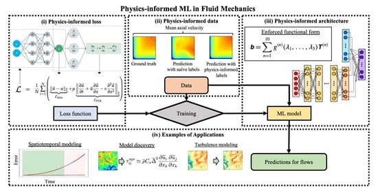
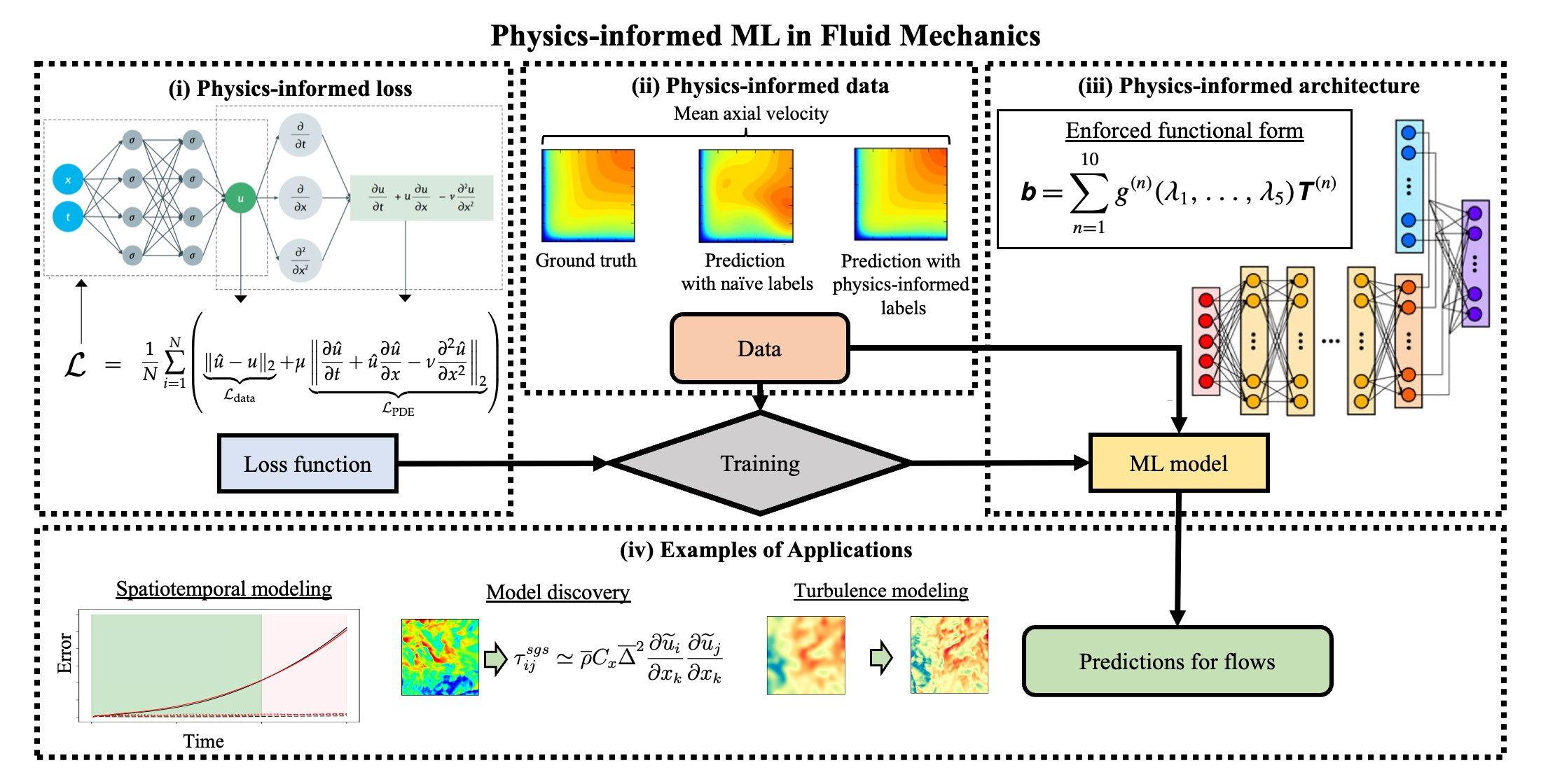
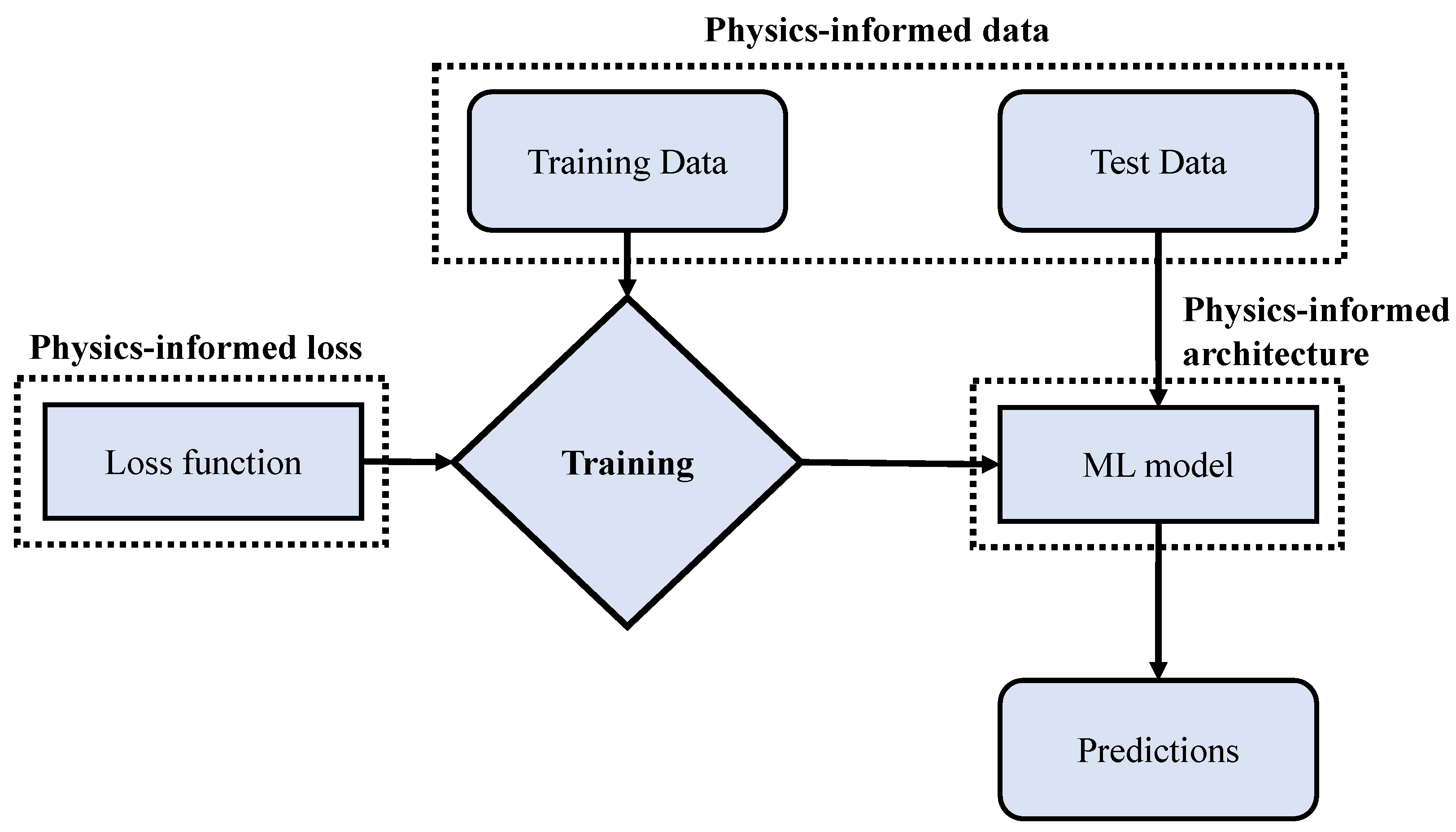
2. Physics-Informed Machine Learning

In this section, we discuss key concepts behind and review existing studies on PIML applied to fluid mechanics problems with a particular focus on challenging configurations. PIML was first proposed as a framework that can account for physical domain knowledge in every stage of ML for improving predictive accuracy in conditions where data are sparse or insufficient [68]. In other words, as can be seen in Figure 2, PIML is formed by embedding domain knowledge into (i) the model input/output, (ii) model loss functions, and (iii) model architecture, which will be discussed in detail in the following sections.

2.1. Physics-Informed Features and Labels

Physics can be embedded into the input data (features) and the model output (labels) through pre-processing steps involving physical intuition, feature selection [69] and extraction [70], as well as mathematical transformations.

The choice of labels can be of particular interest during predictive modeling, as universal approximators, such as ML models, will possess small but significant quantities of approximal error. As such, there has been a significant focus on employing ML models in problems that already possess existing errors—such as with turbulence modeling, where we know errors exist within current analytic models [71,72]. The application of ML to turbulence modeling is popular and has been reviewed extensively by several authors [45,73,74]. Another popular choice of model outputs involves inverse modeling [75], which is the task of obtaining the model parameters from measured data, as we know that conventional CFD solvers cannot be applied effectively in this domain.

Another physics-informed method involves selecting an easily trained form of a label that can be transformed to another desired quantity. For example, Cruz et al. [76] proposed the use of the divergence of the Reynolds stress tensor, i.e., the Reynolds stress vector, as a label, instead of the Reynolds stress tensor. This is based on the observation that errors in the mean velocity arise when inserting the Reynolds stress tensor (extracted from DNS databases) into the mean momentum balance equations. As shown in Figure 3, when demonstrated on a turbulent (Re = 3200) square duct flow, mean velocity fields constructed from the Reynolds stress vector were found to be significantly more accurate than fields constructed from the Reynolds stress tensor.

When dealing with ML features, two competing paradigms can be considered: (i) learning with hand-engineered features, and (ii) representation learning [77], which seeks to develop ML models that can perform well with raw unprocessed data. Physics-informed features belong to the former category. Early ML work on fluid mechanics utilized conventional feature selection techniques without applying domain knowledge. For example, Duraisamy et al. [12] employed the hill-climbing algorithm [78], which works by increasing the size of the feature set until the ML accuracy stops increasing, in an inverse modeling problem for identifying the analytic forms of closure models. Dimensionality reduction techniques such as proper orthogonal decomposition (POD) [79], a popular method in analyzing turbulent flows [80], have also been applied as feature extraction techniques for ML models. For example, Lui and Wolf [81] demonstrated the use of POD for reducing the dimensionality of turbulent airfoil data before training an NN for a reduced-order modeling application.

One of the first works on embedding physical knowledge into ML involves a feature engineering technique by Ling et al. [47]. In this work, the authors embedded rotational invariance and non-dimensionality into features for predicting Reynolds stress anisotropy. This approach showed improvements in predictive accuracy in random forests after feature processing, while the use of untransformed data in NNs resulted in more accurate predictions. Due to the mixed effectiveness these techniques, physics-informed feature techniques are typically applied on a case-by-case basis, and they can benefit from benchmarking, as will be discussed in Section 4. Other concepts can also be embedded into the ML model via feature transformation. For example, Xie et al. [82] transformed the spatial coordinates of features and labels to match coordinates orthogonal to curved surfaces, and they demonstrated an 18% reduction in error when modeling turbulent closure.

2.2. Physics-Informed Architecture

One of the earliest customized ML architectures for fluid mechanics involves the Tensor Basis NN (TBNN) [48], which used a special architecture, shown in Figure 4, for embedding invariance by enforcing a functional form for predicting the Reynolds stress anisotropy tensor. In this a posteriori study, TBNN simulations accurately predicted the occurence of corner vortices, which vanilla ML models failed to predict. Since then, the TBNN has been extended toward problems in turbulent heat transfer [83] as well as improved [84] to consider boundary conditions, non-locality, and Reynolds number embeddings. The TBNN has inspired other architectures such as the Vector Basis Neural Network (VBNN) [85], which has been modified to specifically predict the divergence of the subgrid-scale stresses.

Numerous other architectures have been developed with the similar purpose of enforcing physical, tensorial, and PDE properties via architecture modifications. For example, Frezat et al. [86] enforced linearity, as well as Galilean, rotational and translational invariances, through modifications to a CNN architecture. The resulting ML model demonstrated lower errors than vanilla CNN models. Wang et al. [87] proposed the equivariant NN that introduced symmetries into the ML model predictions. Liu et al. [36] introduced a PDE-preserving NN (PPNN) architecture that demonstrated excellent stability for spatiotemporal predictions. The PPNN works by forming residual connections between input velocities downsampled on the right-hand side (RHS) of the Navier–Stokes equations to result in more stable predictions than a vanilla CNN model. This approach will also be demonstrated in a case study in Section 3. Wang et al. [88] proposed a TurbulentFlowNet (TFNet) architecture consisting of three encoder layers that received three differently filtered input flow fields to account for the multi-scale nature of turbulent flows. The resulting architecture outperformed standard CNN architectures in a 2D turbulent flow configuration. Many of these architectures have been tested on different configurations. Thus, while these studies do demonstrate that PIML techniques can outperform vanilla ML methods, it is still difficult to ascertain the benefits of one PIML approach over another without benchmarking, as will be discussed in Section 4.

In contrast to the architecture-level approaches discussed, the Fourier Neural Operator (FNO) [89] represents a physics-informed architecture method at the layer-wise level. It is based on the Fourier transform, which is a method commonly used in spectral analysis of turbulence and has been demonstrated in a spatiotemporal modeling problem in 2D turbulence configurations. As shown in Figure 5, this operator works by (i) applying Fourier transformation on the inputs, (ii) then applying a linear transformation on the lower spectral modes, and (iii) applying an inverse Fourier transform, before (iv) adding a trainable bias term. The NNs with FNO outperformed traditional ML approaches, demonstrating an 8% error when applied to 2D configuration, with vorticity initialized with a normal distribution at Re = 10,000. This approach outperforms vanilla ML approaches (11% error on U-Net [90] and 23% error on ResNet [9]) and the aforementioned TFNet [88] (with 11% error) on the same configuration. Recently, the FNO was also applied to a 3D LES configuration [91].

2.3. Physics-Informed Loss Functions

A major development in PIML, which deserves extensive discussion due to its proliferation and influence, is the Physics-Informed Neural Network (PINNs), which was first applied to solving a 1D Burgers equation and later applied to solving the Navier–Stokes equations in a 2D flow over a cylinder [25]. For the problem involving the Burgers equation, the PINN could generate spatiotemporal predictions with a $\mathcal{O}\left({10}^{-4}\right)$ mean-squared-error solely with initial and boundary condition data. As with vanilla neural networks, the predictive accuracy of PINN was still found to be dependent on the model’s hyperparameters, and it increased with the amount of training data provided. In the 2D flow over cylinder problem [25], PINNs were demonstrated to predict the pressure and viscosity of the Navier–Stokes equations in an inverse modeling problem. This work differed from the previous studies (which focused on model input, output, and architecture) by introducing soft-constraints in the loss function $\mathcal{L}$:

$$\underset{\theta }{arg\; min}\sum _{i=1}^N\left({\mathcal{L}}_{\mathrm{data}}\left(y_i\right)+\mu {\mathcal{L}}_{\mathrm{k}}(y_i,\theta )\right),$$

(2)

where N is the number of training samples, $\mu$ is a tunable weighting parameter, and ${\mathcal{L}}_k$ contains the k-th constraint, which is related to the partial differential equations (${\mathcal{L}}_{\mathrm{PDE}}$), initial conditions, and boundary conditions. For an example involving the 1D Burgers equation:

$$\begin{array}{c}\hfill {\displaystyle \frac{\partial u}{\partial t}}+u{\displaystyle \frac{\partial u}{\partial x}}=\nu {\displaystyle \frac{{\partial }^{2}u}{\partial x^2}}\end{array}$$

(3)

the loss function in Equation (2) for predicting velocity u with N number of training samples (and viscosity $\nu$) may take the form:

$$\begin{array}{c}\hfill \frac{1}{N}\sum _{i=1}^N\left(\underset{{\mathcal{L}}_{\mathrm{data}}}{\underbrace{{\parallel \widehat{u}-u\parallel }_2}}+\mu \underset{{\mathcal{L}}_{\mathrm{PDE}}}{\underbrace{{∥{\displaystyle \frac{\partial \widehat{u}}{\partial t}}+\widehat{u}{\displaystyle \frac{\partial \widehat{u}}{\partial x}}-\nu {\displaystyle \frac{{\partial }^2\widehat{u}}{\partial x^2}}∥}_2}}\right)\end{array}$$

(4)

where $\widehat{u}$ is the predicted velocity from PINN, the first term of Equation (4) is the velocity mean-squared error (MSE), while the second term represents a residual term that constrains the optimization problem in order to produce a solution that matches (3). The schematic of the PINN architecture for the 1D Burgers equation is depicted in Figure 6.

The PINN framework was later extended to specifically tackle several laminar and incompressible fluid flow problems. This included simulating vortex-induced vibrations [22] and tackling ill-posed inverse fluid mechanics problems through a so-called hidden fluid mechanics framework [26]. Later, the PINN framework was demonstrated to solve the incompressible Navier–Stokes equations in turbulent flow conditions [27]. In this work, two PINN loss functions were suggested based on two forms of the incompressible Navier–Stokes equations: (i) one based on the velocity–pressure (VP) formulation and (ii) another based on the velocity–vorticity (VV) formulation. Both PINN approaches were tested on a range of laminar canonical cases, as well as a turbulent channel flow, with Re $=\mathcal{O}\left({10}^4\right),$ from the Johns Hopkins Turbulent Database [92]. Both forms of the PINN were found to be effective in simulating laminar cases, with less than 1% velocity MSE. However, a ∼10% velocity MSE was obtained when simulating the turbulent channel DNS with the VP-PINN, while the VV-PINN failed to converge for the turbulent cases. Similar accuracies in both laminar and turbulent cases have been reported in another study involving PINNs with RANS-specific loss functions [29]. While PINNs currently struggle to learn predicting turbulent configurations, Jin et al. [27] noted that PINNs were particularly useful for applications outside typical capabilities of traditional CFD solvers, such as inverse modeling, where the authors could predict the flow Reynolds number from a few samples of velocity data.

PINNs have been employed for inverse modeling in experimental fluid mechanics. Cai et al. [28] proposed a PINN-based method to infer the full continuous 3D pressure and velocity fields on an espresso cup from the snapshots of temperature fields obtained from tomographic background-oriented Schlieren (Tomo-BOS) imaging. On the other hand, Eivazi and Vinuesa [93] used noisy experimental measurements to obtain super-resolution of flow field data in time and space using PINN.

PINNs have now influenced approaches in which loss functions are formulated in the following non-exhaustive list of flow problems. Bode et al. [56] modeled the subgrid-scale stresses by adding a continuity residual term $g={\parallel \nabla ·\mathbf{u}\parallel }_2$ to the loss function of a generative adversarial network (GAN) model in a turbulent reacting flow problem. This model, known as physics-informed enhanced super-resolution GAN (PIESR-GAN), optimizes the physics-informed loss, which ensures continuity, along with the adversarial and accuracy loss terms. Jiang et al. [94] also relied on PDE residuals to accurately perform super-resolution on a turbulent Rayleigh–Bernard problem. Sun et al. [95] added a loss term for the subgrid-scale stresses to an MSE loss function for the eddy viscosity in a turbulent airfoil problem. An entropy term was added by Guan et al. [96] in modeling turbulence to 2D homogeneous isotropic turbulence configurations. Laubscher [35] demonstrated significant improvements when predicting temperature, velocity, and species mass fractions when using segregated-network PINN instead of a vanilla PINN on simulations of water vapor in dry air flowing in a 2D rectangular duct.

2.4. Open-Source PIML Resources

In this section, we provide the reader with several open-source resources for conducting PIML research. One of the most popular datasets for studying fluid mechanics, and earliest attempts at providing public access to turbulence data, is the Johns Hopkins Turbulence Database [92]. Xiao et al. [97] has shared parametric geometry DNS of flows over periodic hills, over GitHub and the NASA Langley Turbulence Modeling Portal [98]. Eckert et al. [99] presented one of the first turbulence datasets targeted specifically for ML applications. Bonnet et al. [100] has provided an ML dataset, consisting of airfoil cases, for approximating the RANS solution. To deal with the large cost and size of DNS datasets, crowd-sourcing and public repositories such as Kaggle [101] could be employed to improve access to high-fidelity ML training data. For example, BLASTNet [102], a centralized web platform for indexing DNS data with consistent data formats, has recently been developed. In this approach, members from the research community contribute to individual DNS datasets that are stored in Kaggle repositories (each with $\mathcal{O}\left(100\right)$ GB storage limit), with download links and metadata consolidated in a single webpage for easy accessibility.

Open-source resources are not restricted to publicly accessible datasets. Nvidia Modulus [103], formerly known as SimNet, provides a framework for AI-driven multi-physics simulations, providing access to a wide range of PIML architectures and loss functions as well as simulation modules such as mesh generation, multi-GPU computation, etc. Recently, Wang et al. [104] developed a CFD simulation framework to predict fluid flows with a low-mach approximation on the TPU platform using Tensorflow’s ML package implemented in python. JAXFluids [105] also provides a similar fully integrated framework for fluid simulation modules and ML capabilities. PDEBench [106] presents a benchmark suite that matches with practices from the global ML community. It provides access to popular vanilla (U-Net [90], ResNet [9]) and physics-informed (PINN [25], FNO [89], etc.) architectures, and a set of canonical configurations based on Burgers, as well as incompressible and compressible Navier–Stokes, equations.

3. Case Study: Lid-Driven Cavity

In this section, we demonstrate the effectiveness of physics-informed machine learning algorithms. The most popular PIML model is the PINN, which has already been shown to be effective for several fluid flow problems. Therefore, we decided to choose a different PIML model, i.e., the PDE-preserving neural network (PPNN). As opposed to PINN, where the physical constraints are embedded in the form of a loss function, in PPNN, the PDE structures are preserved by modifying the model architecture itself with the use of residual connections. The utility of PPNN [36] has previously been demonstrated in terms of training complexity and extrapolability for a few spatiotemporal dynamic problems. Here, we use the PPNN approach to reconstruct the 2D flow fields of a lid-driven cavity problem. Our objective is to assess the advantages of using PIML models over baseline vanilla ML models in terms of long-term prediction and generalizability, especially for unseen parameter spaces.

3.1. Problem Setup

We consider the 2D lid-driven cavity problem at different Reynolds numbers ($\mathrm{Re}$). The data for training and validation are generated by solving the Navier–Stokes equation numerically using a finite difference (FD) scheme. The governing equations are:

$$\begin{array}{cc}\hfill \frac{\partial \mathit{u}}{\partial t}+\mathit{u}·\nabla \mathit{u}& =-\nabla p+\frac{1}{\mathrm{Re}}{\nabla }^2\mathit{u}\hfill \\ \hfill \nabla ·\mathit{u}& =0\hfill \end{array}$$

(5)

where $\mathit{u}={[u(x,y,t),v(x,y,t)]}^T$ is the velocity vector, and $p(x,y,t)$ is the pressure. The length of the computational domain is unity in both directions. The velocity of the lid is considered to be $u_{\mathrm{top}}=1$. No-slip condition is enforced at the other three boundaries. Neumann boundary conditions are applied for the pressure at all boundaries. Four different Reynolds numbers are considered for this study: 400, 500, 600 and 750. In all cases, the velocity and pressure fields are generated using the FD solver for 5000 numerical steps with a time step of $\Delta t=0.01$. A uniform Cartesian mesh with $100\times 100$ is used in the numerical solver.

The training dataset involves 100 snapshots from only two $\mathrm{Re}$, i.e., 500 and 750. These snapshots are collected every 20 numerical steps to form the training trajectory, which means the learning step is set as $\tau =20\Delta t=0.2$. Thus, the training set covers a total time of $T=100\tau$. The trained model is then used to predict the flow field for the other $\mathrm{Re}$, i.e., 400 (extrapolation) and 600 (interpolation), which are not part of the training set. The PPNN-specific training and prediction parameters are described in the following sections.

3.2. Implementation of PPNN

The PPNN architecture involves two components: a trainable baseline convolutional residual network and a PDE-preserving part. Both of them are connected in an encoder–decoder fashion. In the PDE-preserving part, the governing PDEs are constructed based on convolution operators defined by FD stencils. A bilinearly downsampled input flow field starting from the high-resolution data at time t is used as input to the PDE-preserving part. The use of both convolution operators and low-resolution grid reduces the computational overhead significantly during the model prediction. The low-resolution output from the PDE-preserving part at time $t+\Delta t$ is then upsampled using bicubic upsampling. The high-resolution flow field at t along with the upsampled flow field information from the PDE-preserved portion at $t+\Delta t$ are then used as input channels in the trainable part of the PPNN. The conceptual schematic and detailed implementation of the PPNN model are reproduced in Figure 7 from the original paper [36]. The same architecture from the paper is used in this study, which includes two convolutional layers with $6\times 6$ kernel, zero padding and a stride of 2, which was followed by four ConvResNet blocks. Each block has a $7\times 7$ kernel, 96 channels and zero padding of 3. Finally, the decoder part includes pixelshuffle with an upscale factor of 4 along with a convolutional layer of $5\times 5$ kernel and zero padding of 2. An additional input channel is included to map the physical parameter, which is only $\mathrm{Re}$ in this case, to the flow field. More details regarding the implementation of PPNN are available in Liu et al. [36].

3.3. Results and Discussion

To demonstrate the advantage of using prior knowledge in an existing ML framework, we have used two different versions of PPNN: (i) preserving full Navier–Stokes equation, where each term in Equation (5) is constructed based on convolution operators (as shown in Figure 7), and (ii) preserving partial Navier–Stokes equation, where all terms except the first term of RHS ($\nabla p$) are embedded in a similar fashion. Solving real-world applications using traditional numerical simulation methods is a great challenge, as the underlying physics behind a phenomena may not be fully understood or the governing equations could only be partially known. The second version of the PPNN is chosen to investigate the impact of providing this partial knowledge to the data-driven model. Both PPNN predictions are compared to the high-resolution FD numerical solutions as a reference. The error at each time step, ${ϵ}_t$ at time t, is defined as:

$${ϵ}_t=\frac{\left|\right|{\mathit{u}}_t\left({\lambda }_i\right)-({\widehat{\mathit{u}}}_{t-1}+f_{\theta }({\widehat{\mathit{u}}}_{t-1},{\lambda }_i|\tilde{\theta })){\left|\right|}_2}{\left|\right|{\mathit{u}}_t\left({\lambda }_i\right){\left|\right|}_2}$$

(6)

where ${\mathit{u}}_t\left({\lambda }_i\right)$ is the velocity magnitude of the reference solution at time t for the physical parameter, ${\lambda }_i$ (which corresponds to the i-th $\mathrm{Re}$ in this case), and $f_{\theta }$ represents the trained NN update with weights $\tilde{\theta }$. The predicted solution by PPNN at time $t-\Delta t$ is denoted by ${\widehat{\mathit{u}}}_{t-\Delta t}$ and evaluated as

$$\begin{array}{cc}\hfill {\widehat{\mathit{u}}}_t& ={\widehat{\mathit{u}}}_{t-\Delta t}+f_{\theta }({\widehat{\mathit{u}}}_{t-\Delta t},{\lambda }_i|\tilde{\theta })\forall t\in [2,n]\hfill \\ \hfill {\widehat{\mathit{u}}}_1& ={\mathit{u}}_0\left({\lambda }_i\right)+f_{\theta }({\mathit{u}}_0\left({\lambda }_i\right),{\lambda }_i|\tilde{\theta })\hfill \end{array}$$

(7)

where n is the number of evolving steps starting from the initial high-resolution solution field, ${\mathit{u}}_0$. The relative testing errors of the magnitude of velocity corresponding to the prediction of PPNN, PPNN-partial and baseline ConvResNet model compared to the ground truth reference are shown in Figure 8. Clearly, the prediction of the baseline model suffers from error accumulation, which is a well-established problem within auto-regressive models. However, the physics-informed ML model, PPNN, suppresses the error accumulation and outperforms the baseline model by providing accurate predictions of the velocity field even beyond the training period ($t>T$) for $\mathrm{Re}=500$ and 750. In case of unseen conditions ($\mathrm{Re}=400$ and 600), PPNN shows very low roll-out errors compared to the baseline model. Even for PPNN-partial cases for both training and test $\mathrm{Re}$, the preservation of partially known PDE structures outperforms the vanilla ConvResNet model. Although there is an error for $\mathrm{Re}=400$ and 600, PPNN-partial exhibits a larger error than fully known PDE preserved PPNN, the error never accumulates, and it provides a stable and reasonably accurate solution.

To emphasize the advantage of PPNN even further, the contours of the velocity field prediction from PPNN, PPNN-partial and the baseline model along with ground truth are shown in Figure 9 for $\mathrm{Re}=400$. Both PPNN predictions emulate the ground truth accurately which is consistent with the error plot (Figure 8). In contrast, despite accurate predictions from the baseline model during the few initial timesteps, error rapidly accumulates to provide random, noisy and unphysical solution field. Overall, PPNN (an example of a PIML approach) demonstrates significantly better generalizability, stability and robustness in terms of long-term prediction than the baseline (vanilla) ML model.

4. Challenges and Opportunities

PIML has been developed with the overarching goal of improving the generalizability of model predictions outside of relatively small fluid mechanics datasets employed to train ML models. While studies so far have demonstrated that many of the existing PIML approaches can have benefits over vanilla ML approaches, physics-informed approaches in fluid mechanics (especially in turbulent flow problems) can still be advanced as this set of techniques matures. Having discussed the existing literature and demonstrated the utility of PIML in fluid mechanics, we conclude this review with a set of recommendations for readers interested in advancing this field. This includes (i) benchmarking, (ii) optimization, (iii) new algorithms and applications, and (iv) limitations in predicting complex flow configurations. These topics are tailored for PIML in fluid mechanics. We have provided a more general discussion on ML in reacting/non-reacting flows on broader ranging challenges and opportunities, such as interpretability, uncertainty quantification, and computational complexity in another review paper [61].

4.1. Benchmarking Existing PIML Methods

One of the largest challenges in ML is differentiating the benefits of competing methods, since the superior performance of specific ML methods can be highly dependent on the problem statement, configuration, and dataset. This is one reason that many ML practitioners still rely on hyperparameter searches [107] to identify the most suitable algorithm, architecture, and parameters when applying ML to a new problem. As such, it is currently not entirely clear whether physics-informed features, labels, architectures, and loss functions outperform competing ML paradigms, especially since PIML methods have been demonstrated to be ineffective and even harmful in certain test conditions [108]. Fortunately, this is a challenge that can be addressed as ML in fluid mechanics begins to mature. To overcome this challenge, mature ML fields (such as computer vision and natural language processing (NLP)) have established a culture of benchmarking hundreds of popular strategies through competitions [10,109] on community-established datasets. This culture could be emulated for fluid mechanics studies, which would result in numerous benchmark studies for the fluid mechanics community. However, significant strides in (i) forming community-accepted datasets [102] and (ii) organizing a community-wide benchmarking study will need to be accomplished before such a challenge can be met. Numerous efforts discussed in Section 2.4 present a step toward addressing these challenges.

4.2. Optimization and Loss

Many of the ideas that have led to the development of physics-informed loss functions have existed prior to the contemporary proliferation of ML techniques. For example, the idea of constraining neural networks for scientific modeling have existed since 1992, when Psichogios and Ungar [110] trained a custom loss function formulated from differential equations that governed a bioreactor model. Results from this model showed higher accuracy, generalization properties, and training data efficiency than conventional NNs. As such, there is an abundance of ML literature that can inspire advancements physics-informed loss approaches.

From a more conventional ML perspective, the use of physics-informed loss functions is highly related to the practice of regularization [111], which is typically used to address overfitting. Overfitting occurs when an ML model can predict accurately when fed with inputs from the training set, but it predicts poorly when fed with inputs from outside the training set. Conventional forms of regularization would involve the use of the $L_2$-norm and $L_1$-norm of model weight W, i.e., ${\parallel W\parallel }_2$ and ${\parallel W\parallel }_1$, respectively. The minimization of the $L_2$-norm results in evenly distributed weights with small magnitudes, and thus, it reduces model complexity when fully trained, while minimization of the $L_1$-norm encourages the formation of zero-value model weights and thus results in sparse ML models. Hence, from a regularization perspective, PINNs could be viewed as NNs that have been regularized by domain knowledge to generalize to out-of-distribution samples with the same governing PDEs/ODEs.

Analysis from a regularization perspective has successfully revealed important properties of PINNs [108]. PINN regularization differs from the aforementioned norm regularization, as norm functions are convex. In contrast, physics-informed loss functions are not guaranteed to be convex, while the introduction of differential operators to the loss function could result in an ill-conditioned problem during training. Krishnapriyan et al. [108] demonstrated that these challenges in optimization could result in PINNs with 100% error even in simple advection problems. However, the authors also demonstrated that several strategies could be employed for overcoming these issues in optimization. Firstly, a warm start-up approach (which involves training a PINN on a simple problem before progressively training the same network on more complex configurations) was demonstrated to alleviate this optimization issue. Secondly, the authors demonstrated that PINNs were more suited for sequence modeling (where solutions in a late timestep are predicted from solutions from a previous timestep) as opposed to previous work [25] that focused on predicting the entire spatiotemporal solution at once from initial/boundary conditions.

This work demonstrates that the physics-informed loss function can benefit from studies in related fields where ML models are applied in many tasks (multi-task learning [112]) and multiple objectives (multi-objective optimization [113]), which have been studied extensively from a theoretical viewpoint and applied to practical systems in robotics, computer vision, and NLP. Since PINNs and physics-informed loss functions are relatively new, advancements in this direction have been fairly recent.

4.3. Embedding Physics to New Algorithms and Applications

One of the largest challenges for ML research is the fast-moving pace and wide-ranging nature of the field. For example, in computer vision, GANs [114] (alongside its variants) were widely held as the best model for generative ML, but recently, diffusion probabilistic models [115] have become much more popular [116]. As such, there are many opportunities to extend the PIML framework to new algorithms that have been developed for applications outside of fluid mechanics.

This is especially true since PIML developments in other scientific and engineering fields can be demonstrated and modified for predicting flow fields. For example, PINNs that have been developed for solving problems in chemical kinetics could be extended to the study of reacting flows. One of these developments includes the Stiff-PINN [33], which first treats species with faster time scales, i.e., quasi-steady species (QSS), before treating the rest of the species with a standard PINN. Similarly, Weng and Zhou [34] proposed the multiscale PINN (MPINN), which forms clusters of species based on their time scales and then trains separate NNs with the individual clusters. These are a non-exhaustive list of PINN variants that should be explored on different flow configurations.

We note that while this review has mostly focused on supervised learning due to their popularity within ML research, PIML could be employed toward unsupervised algorithms and semi-supervised algorithms, which have not been studied as extensively when compared to studies involving NNs. For example, Baddoo et al. [117] introduced physics-informed dynamic mode decomposition that introduced constraints based on conservation, self-adjointness, localization, causality, and shift invariance. The method outperformed the vanilla dimensionality reduction technique [118] on a wide range of PDE problems, including a transitional channel flow configuration. In another example, Liu and Wang [119] developed a physics-informed deep reinforcement learning system by introducing governing differential equations to loss functions of a model-based RL system. This approach outperformed vanilla algorithms when applied to a control problem involving viscous Burgers equation.

4.4. Limitations in Predicting Complex Configurations

Throughout this review, we have noted that while PIML methods have demonstrated low errors in laminar configurations, errors in turbulent flows are often orders of magnitude higher in comparison due to problems tied to (i) non-linearity, (ii) high-dimensionality, and (iii) multi-scale physics. More extensive studies will be needed to identify specific ML approaches that can address these issues before the merits of physics-informed approaches can be rigorously evaluated. An extensive study [120] involving seven different deep learning architectures revealed errors ranging from 1 to 20% error (depending on the architecture used) in the velocity spectra when predicting the temporal evolution of 3D-filtered compressible homogeneous isotropic turbulence. This study provides recommendations in choosing specific deep learning layers and pre-processing the data (such as data augmentation [121] through Gaussian noise and the use of dilated convolutional layers [122]) for minimizing errors in turbulent flows, which can be emulated in studies focused on challenging turbulent regimes.

As PIML matures, these techniques will eventually be employed to modeling and studying realistic configurations found in environmental and industrial settings, which offer additional challenges tied to (i) complex geometries as well as (ii) poorly understood multi-physics phenomena. Promising techniques for treating configurations with complex geometries include architectures specialized for unstructured data such as graph neural networks (GNNs) [123], which have already been demonstrated for flow prediction problems on a wide range of mesh geometries [124]. He et al. [125] highlighted the suitability of this method over conventional ML methods by demonstrating that the velocity flow fields predicted by GNNs (6% error) outperformed conventional feedforward and CNN architectures (16% and 42% error, respectively) when comparing force coefficients evaluated from those flow fields in a 2D unstructured configuration of flow-over-a-cylinder over multiple $\mathrm{Re}$.

In many realistic flow problems, multi-physics phenomena (such as those found in non-Newtonian, multi-phase, trans-/super-critical, and hypersonic flows) are still not well understood, which can introduce uncertainty when developing predictive models and simulations. This can introduce limitations in availability of high-quality data, since the training data could be obfuscated by inaccurate assumptions/observations. Here, PIML methods should be combined with algorithms that can measure the uncertainty of their predictions, such as Gaussian Process Regression [126] and Bayesian neural networks [127]. Physics-informed versions of these models have been applied to generic PDE problems [128] and can be extended toward these challenging flow configurations. In addition to limitations, these poorly understood configurations include opportunities to combine domain expertise with knowledge discovery algorithms. An example of this involves the modeling turbulent phenomena within trans-/super-critical flows, which can introduce uncertainty to traditional turbulence modeling approaches due to new closure terms that can arise from nonlinear thermodynamic and transport properties. Here, domain knowledge can be employed to reduce the computational cost of symbolic regression methods (through reduction of the search space) to discover new closure models from DNS data, which have been performed in previous studies [24,129]. These sets of methods could be extended for model discovery applications in other poorly understood flow configurations.

5. Conclusions

In this article, we have reviewed the physics-informed ML techniques for applications within fluid flow problems. The general idea behind PIML models is to integrate domain knowledge and/or the information about the governing PDEs with the deep NN models. Incorporating these aspects with traditional ML algorithms have resulted in better and more stable prediction accuracy, faster training and improved generalizability. Thus, the successful embedding of physical knowledge, either as input features/labels or in the form of a modified loss function or by preserving the PDE structures in the model architecture itself, holds exciting promise for the advancement of solving fluid flows, especially complex turbulent flows. Here, we have highlighted the applications of PIML in the field of fluid mechanics, ranging from knowledge discovery, prediction of spatiotemporal dynamics in different flow configurations, as well as super-resolution and turbulent closure modeling. We also demonstrate the utility of a PIML algorithm through a standard fluid flow problem.

Fluid mechanics is a data-rich field that is founded on physical concepts encapsulating conservation relations. Relying solely on the data-driven methods may omit these concepts, as data-driven methods could ignore certain physical constraints or conservation principles. Therefore, fluid mechanics problems can be an excellent testbed for developing novel PIML algorithms. While PIML approaches have demonstrated significant progress in fluid flow problems, several open questions and opportunities still exist. As each PIML model has only been demonstrated on particular problem configurations and datasets, benchmarking existing PIML methods is still an open challenge, which will need to be addressed as ML within fluid mechanics matures. It is also important to keep track of the fast-moving and mercurial developments of ML outside fluid mechanics. In these domains, new innovations are introduced at a rapid pace, leaving many existing methods obsolete. Researchers should take inspiration from these developments either to improve specfic components of existing PIML models (such as optimization routines and loss functions) or to develop entirely new algorithms for resolving existing challenges within flow problems. As PIML development continues to progress, this set of approaches is expected to play a significant role in the offering computationally efficient predictive models to fluid mechanics that could be more reliable than their vanilla counterparts, especially in complex flow configurations.

References

1. Karniadakis, G.E.; Kevrekidis, I.G.; Lu, L.; Perdikaris, P.; Wang, S.; Yang, L. Physics-informed machine learning. Nat. Rev. Phys. 2021, 3, 422–440. [Google Scholar] [CrossRef]
2. Bishop, C.M. Pattern Recognition and Machine Learning; Springer: Berlin, Germany, 2006. [Google Scholar]
3. Nair, V.; Hinton, G.E. Rectified linear units improve restricted Boltzmann machines. Proc. Int. Conf. Mach. Learn. 2010, 27, 807–814. [Google Scholar]
4. Amari, S.i. Backpropagation and stochastic gradient descent method. Neurocomputing 1993, 5, 185–196. [Google Scholar] [CrossRef]
5. Rumelhart, D.E.; Hinton, G.E.; Williams, R.J. Learning representations by back-propagating errors. Nature 1986, 323, 533–536. [Google Scholar] [CrossRef]
6. LeCun, Y.; Bottou, L.; Bengio, Y.; Haffner, P. Gradient-based learning applied to document recognition. Proc. IEEE 1998, 86, 2278–2324. [Google Scholar] [CrossRef] [Green Version]
7. Mnih, V.; Kavukcuoglu, K.; Silver, D.; Graves, A.; Antonoglou, I.; Wierstra, D.; Riedmiller, M. Playing Atari with deep reinforcement learning. arXiv 2013, arXiv:1312.5602. [Google Scholar]
8. Mnih, V.; Kavukcuoglu, K.; Silver, D.; Rusu, A.A.; Veness, J.; Bellemare, M.G.; Graves, A.; Riedmiller, M.; Fidjeland, A.K.; Ostrovski, G.; et al. Human-level control through deep reinforcement learning. Nature 2015, 518, 529–533. [Google Scholar]
9. He, K.; Zhang, X.; Ren, S.; Sun, J. Deep residual learning for image recognition. In Proceedings of the IEEE Conference on Computer Vision and Pattern Recognition (CVPR), Las Vegas, NV, USA, 27–30 June 2016; pp. 770–778. [Google Scholar]
10. Russakovsky, O.; Deng, J.; Su, H.; Krause, J.; Satheesh, S.; Ma, S.; Huang, Z.; Karpathy, A.; Khosla, A.; Bernstein, M.; et al. ImageNet large scale visual recognition challenge. Int. J. Comput. Vis. 2015, 115, 211–252. [Google Scholar]
11. Tracey, B.D.; Duraisamy, K.; Alonso, J.J. A machine learning strategy to assist turbulence model development. In Proceedings of the 53rd AIAA Aerospace Sciences Meeting, Kissimmee, FL, USA, 5–9 January 2015; p. 1287. [Google Scholar]
12. Duraisamy, K.; Zhang, Z.J.; Singh, A.P. New approaches in turbulence and transition modeling using data-driven techniques. In Proceedings of the 53rd AIAA Aerospace Sciences Meeting, Kissimmee, FL, USA, 5–9 January 2015; p. 1284. [Google Scholar]
13. Jolliffe, I.T.; Cadima, J. Principal component analysis: A review and recent developments. Philos. Trans. Royal Soc. A 2016, 374, 20150202. [Google Scholar] [CrossRef] [PubMed] [Green Version]
14. Jain, A.K. Data clustering: 50 years beyond K-means. Pattern Recognit. Lett. 2010, 31, 651–666. [Google Scholar] [CrossRef]
15. Reddy, G.; Celani, A.; Sejnowski, T.J.; Vergassola, M. Learning to soar in turbulent environments. Proc. Natl. Acad. Sci. USA 2016, 113, E4877–E4884. [Google Scholar] [CrossRef] [Green Version]
16. Novati, G.; de Laroussilhe, H.L.; Koumoutsakos, P. Automating turbulence modelling by multi-agent reinforcement learning. Nat. Mach. Intell. 2021, 3, 87–96. [Google Scholar] [CrossRef]
17. Fukami, K.; Fukagata, K.; Taira, K. Super-resolution reconstruction of turbulent flows with machine learning. J. Fluid Mech. 2019, 870, 106–120. [Google Scholar] [CrossRef] [Green Version]
18. Wang, Z.; Chen, J.; Hoi, S.C. Deep learning for image super-resolution: A survey. IEEE Trans. Pattern Anal. Mach. Intell. 2020, 43, 3365–3387. [Google Scholar] [CrossRef] [PubMed] [Green Version]
19. Maulik, R.; San, O.; Jacob, J.D.; Crick, C. Sub-grid scale model classification and blending through deep learning. J. Fluid Mech. 2019, 870, 784–812. [Google Scholar] [CrossRef] [Green Version]
20. Chung, W.T.; Mishra, A.A.; Perakis, N.; Ihme, M. Data-assisted combustion simulations with dynamic submodel assignment using random forests. Combust. Flame 2021, 227, 172–185. [Google Scholar] [CrossRef]
21. Li, B.; Yang, Z.; Zhang, X.; He, G.; Deng, B.Q.; Shen, L. Using machine learning to detect the turbulent region in flow past a circular cylinder. J. Fluid Mech. 2020, 905, A10. [Google Scholar] [CrossRef]
22. Raissi, M.; Wang, Z.; Triantafyllou, M.S.; Karniadakis, G.E. Deep learning of vortex-induced vibrations. J. Fluid Mech. 2019, 861, 119–137. [Google Scholar] [CrossRef] [Green Version]
23. Callaham, J.L.; Rigas, G.; Loiseau, J.C.; Brunton, S.L. An empirical mean-field model of symmetry-breaking in a turbulent wake. Sci. Adv. 2022, 8, eabm4786. [Google Scholar] [CrossRef]
24. Chung, W.T.; Mishra, A.A.; Ihme, M. Interpretable data-driven methods for subgrid-scale closure in LES for transcritical LOX/GCH4 combustion. Combust. Flame 2022, 239, 111758. [Google Scholar] [CrossRef]
25. Raissi, M.; Perdikaris, P.; Karniadakis, G. Physics-informed neural networks: A deep learning framework for solving forward and inverse problems involving nonlinear partial differential equations. J. Comp. Phys. 2019, 378, 686–707. [Google Scholar] [CrossRef]
26. Raissi, M.; Yazdani, A.; Karniadakis, G.E. Hidden fluid mechanics: Learning velocity and pressure fields from flow visualizations. Science 2020, 367, 1026–1030. [Google Scholar] [CrossRef]
27. Jin, X.; Cai, S.; Li, H.; Karniadakis, G.E. NSFnets (Navier-Stokes flow nets): Physics-informed neural networks for the incompressible Navier-Stokes equations. J. Comp. Phys. 2021, 426, 109951. [Google Scholar] [CrossRef]
28. Cai, S.; Wang, Z.; Fuest, F.; Jeon, Y.J.; Gray, C.; Karniadakis, G.E. Flow over an espresso cup: Inferring 3-D velocity and pressure fields from tomographic background oriented Schlieren via physics-informed neural networks. J. Fluid Mech. 2021, 915, A102. [Google Scholar] [CrossRef]
29. Eivazi, H.; Tahani, M.; Schlatter, P.; Vinuesa, R. Physics-informed neural networks for solving Reynolds-averaged Navier–Stokes equations. Phys. Fluids 2022, 34, 075117. [Google Scholar] [CrossRef]
30. Wang, H.; Liu, Y.; Wang, S. Dense velocity reconstruction from particle image velocimetry/particle tracking velocimetry using a physics-informed neural network. Phys. Fluids 2022, 34, 017116. [Google Scholar] [CrossRef]
31. Qiu, R.; Huang, R.; Xiao, Y.; Wang, J.; Zhang, Z.; Yue, J.; Zeng, Z.; Wang, Y. Physics-informed neural networks for phase-field method in two-phase flow. Phys. Fluids 2022, 34, 052109. [Google Scholar] [CrossRef]
32. Aliakbari, M.; Mahmoudi, M.; Vadasz, P.; Arzani, A. Predicting high-fidelity multiphysics data from low-fidelity fluid flow and transport solvers using physics-informed neural networks. Int. J. Heat Fluid Flow 2022, 96, 109002. [Google Scholar] [CrossRef]
33. Ji, W.; Qiu, W.; Shi, Z.; Pan, S.; Deng, S. Stiff-PINN: Physics-informed neural network for stiff chemical kinetics. J. Phys. Chem. A 2021, 125, 8098–8106. [Google Scholar] [CrossRef] [PubMed]
34. Weng, Y.; Zhou, D. Multiscale physics-informed neural networks for stiff chemical kinetics. J. Phys. Chem. A 2022, 126, 8534–8543. [Google Scholar] [CrossRef]
35. Laubscher, R. Simulation of multi-species flow and heat transfer using physics-informed neural networks. Phys. Fluids 2021, 33, 087101. [Google Scholar] [CrossRef]
36. Liu, X.Y.; Sun, H.; Zhu, M.; Lu, L.; Wang, J.X. Predicting parametric spatiotemporal dynamics by multi-resolution PDE structure-preserved deep learning. arXiv 2022, arXiv:2205.03990. [Google Scholar]
37. Ren, P.; Rao, C.; Liu, Y.; Wang, J.X.; Sun, H. PhyCRNet: Physics-informed convolutional-recurrent network for solving spatiotemporal PDEs. Comput. Methods Appl. Mech. Eng. 2022, 389, 114399. [Google Scholar] [CrossRef]
38. Kochkov, D.; Smith, J.A.; Alieva, A.; Wang, Q.; Brenner, M.P.; Hoyer, S. Machine learning-accelerated computational fluid dynamics. Proc. Natl. Acad. Sci. USA 2021, 118, e2101784118. [Google Scholar] [CrossRef] [PubMed]
39. De Avila Belbute-Peres, F.; Economon, T.; Kolter, Z. Combining differentiable PDE solvers and graph neural networks for fluid flow prediction. In Proceedings of the 37th International Conference on Machine Learning, Virtual, 13–18 July 2020; pp. 2402–2411. [Google Scholar]
40. Um, K.; Brand, R.; Fei, Y.R.; Holl, P.; Thuerey, N. Solver-in-the-loop: Learning from differentiable physics to interact with iterative PDE-solvers. Adv. Neural Inf. Process. Syst. 2020, 33, 6111–6122. [Google Scholar]
41. Gao, H.; Sun, L.; Wang, J.X. PhyGeoNet: Physics-informed geometry-adaptive convolutional neural networks for solving parameterized steady-state PDEs on irregular domain. J. Comp. Phys. 2021, 428, 110079. [Google Scholar] [CrossRef]
42. Geneva, N.; Zabaras, N. Modeling the dynamics of PDE systems with physics-constrained deep auto-regressive networks. J. Comp. Phys. 2020, 403, 109056. [Google Scholar] [CrossRef] [Green Version]
43. Ranade, R.; Hill, C.; Pathak, J. DiscretizationNet: A machine-learning based solver for Navier–Stokes equations using finite volume discretization. Comput. Methods Appl. Mech. Eng. 2021, 378, 113722. [Google Scholar] [CrossRef]
44. Rao, C.; Sun, H.; Liu, Y. Embedding physics to learn spatiotemporal dynamics from sparse data. arXiv 2021, arXiv:2106.04781. [Google Scholar]
45. Duraisamy, K.; Iaccarino, G.; Xiao, H. Turbulence Modeling in the Age of Data. Annu. Rev. Fluid Mech. 2019, 51, 357–377. [Google Scholar] [CrossRef] [Green Version]
46. Ling, J.; Templeton, J. Evaluation of machine learning algorithms for prediction of regions of high Reynolds averaged Navier-Stokes uncertainty. Phys. Fluids 2015, 27, 085103. [Google Scholar] [CrossRef]
47. Ling, J.; Jones, R.; Templeton, J. Machine learning strategies for systems with invariance properties. J. Comp. Phys. 2016, 318, 22–35. [Google Scholar] [CrossRef] [Green Version]
48. Ling, J.; Kurzawski, A.; Templeton, J. Reynolds averaged turbulence modelling using deep neural networks with embedded invariance. J. Fluid Mech. 2016, 807, 155–166. [Google Scholar] [CrossRef]
49. Parish, E.J.; Duraisamy, K. A paradigm for data-driven predictive modeling using field inversion and machine learning. J. Comp. Phys. 2016, 305, 758–774. [Google Scholar] [CrossRef] [Green Version]
50. Xiao, H.; Wu, J.L.; Wang, J.X.; Sun, R.; Roy, C. Quantifying and reducing model-form uncertainties in Reynolds-averaged Navier-Stokes simulations: A data-driven, physics-informed Bayesian approach. J. Comp. Phys. 2016, 324, 115–136. [Google Scholar] [CrossRef] [Green Version]
51. Singh, A.P.; Medida, S.; Duraisamy, K. Machine-learning-augmented predictive modeling of turbulent separated flows over airfoils. AIAA J. 2017, 55, 2215–2227. [Google Scholar] [CrossRef] [Green Version]
52. Wang, J.X.; Wu, J.L.; Xiao, H. Physics-informed machine learning approach for reconstructing Reynolds stress modeling discrepancies based on DNS data. Phys. Rev. Fluids 2017, 2, 034603. [Google Scholar] [CrossRef] [Green Version]
53. Lapeyre, C.J.; Misdariis, A.; Cazard, N.; Veynante, D.; Poinsot, T. Training convolutional neural networks to estimate turbulent sub-grid scale reaction rates. Combust. Flame 2019, 203, 255–264. [Google Scholar] [CrossRef] [Green Version]
54. Beck, A.; Flad, D.; Munz, C.D. Deep neural networks for data-driven LES closure models. J. Comp. Phys. 2019, 398, 108910. [Google Scholar] [CrossRef] [Green Version]
55. Maulik, R.; San, O. A neural network approach for the blind deconvolution of turbulent flows. J. Fluid Mech. 2017, 831, 151–181. [Google Scholar] [CrossRef] [Green Version]
56. Bode, M.; Gauding, M.; Lian, Z.; Denker, D.; Davidovic, M.; Kleinheinz, K.; Jitsev, J.; Pitsch, H. Using physics-informed enhanced super-resolution generative adversarial networks for subfilter modeling in turbulent reactive flows. Proc. Combust. Inst. 2021, 38, 2617–2625. [Google Scholar] [CrossRef]
57. Kutz, J.N. Deep learning in fluid dynamics. J. Fluid Mech. 2017, 814, 1–4. [Google Scholar] [CrossRef] [Green Version]
58. Brunton, S.L.; Noack, B.R.; Koumoutsakos, P. Machine learning for fluid mechanics. Annu. Rev. Fluid Mech. 2020, 52, 477–508. [Google Scholar] [CrossRef] [Green Version]
59. Brunton, S.L. Applying machine learning to study fluid mechanics. Acta Mech. Sin. 2022, 37, 1–9. [Google Scholar] [CrossRef]
60. Zhu, L.T.; Chen, X.Z.; Ouyang, B.; Yan, W.C.; Lei, H.; Chen, Z.; Luo, Z.H. Review of machine learning for hydrodynamics, transport, and reactions in multiphase flows and reactors. Ind. Eng. Chem. Res. 2022, 61, 9901–9949. [Google Scholar] [CrossRef]
61. Ihme, M.; Chung, W.T.; Mishra, A.A. Combustion machine learning: Principles, progress and prospects. Prog. Energy Combust. Sci. 2022, 91, 101010. [Google Scholar] [CrossRef]
62. Zhou, L.; Song, Y.; Ji, W.; Wei, H. Machine learning for combustion. Energy AI 2022, 7, 100128. [Google Scholar] [CrossRef]
63. Echekki, T.; Farooq, A.; Ihme, M.; Sarathy, S.M. Machine Learning for Combustion Chemistry. In Machine Learning and Its Application to Reacting Flows: ML and Combustion; Springer International Publishing: Cham, Switzerland, 2023; pp. 117–147. [Google Scholar]
64. Zhong, S.; Zhang, K.; Bagheri, M.; Burken, J.G.; Gu, A.; Li, B.; Ma, X.; Marrone, B.L.; Ren, Z.J.; Schrier, J.; et al. Machine learning: New ideas and tools in environmental science and engineering. Environ. Sci. Technol. 2021, 55, 12741–12754. [Google Scholar] [CrossRef]
65. Willard, J.; Jia, X.; Xu, S.; Steinbach, M.; Kumar, V. Integrating scientific knowledge with machine learning for engineering and environmental systems. ACM Comput. Surv. 2022, 55, 1–37. [Google Scholar] [CrossRef]
66. Hao, Z.; Liu, S.; Zhang, Y.; Ying, C.; Feng, Y.; Su, H.; Zhu, J. Physics-informed machine learning: A survey on problems, methods and applications. arXiv 2022, arXiv:2211.08064. [Google Scholar]
67. Cai, S.; Mao, Z.; Wang, Z.; Yin, M.; Karniadakis, G.E. Physics-informed neural networks (PINNs) for fluid mechanics: A review. Acta Mech. Sin. 2022, 37, 1–12. [Google Scholar] [CrossRef]
68. Wu, J.L.; Wang, J.X.; Xiao, H.; Ling, J. A priori assessment of prediction confidence for data-driven turbulence modeling. Flow Turbul. Combust. 2017, 99, 25–46. [Google Scholar] [CrossRef] [Green Version]
69. Li, J.; Cheng, K.; Wang, S.; Morstatter, F.; Trevino, R.P.; Tang, J.; Liu, H. Feature selection: A data perspective. ACM Comput. Surv. 2017, 50, 1–45. [Google Scholar] [CrossRef] [Green Version]
70. Ding, S.; Zhu, H.; Jia, W.; Su, C. A survey on feature extraction for pattern recognition. Artif. Intell. Rev. 2012, 37, 169–180. [Google Scholar] [CrossRef]
71. Germano, M.; Piomelli, U.; Moin, P.; Cabot, W.H. A dynamic subgrid-scale eddy viscosity model. Phys. Fluids A 1991, 3, 1760–1765. [Google Scholar] [CrossRef] [Green Version]
72. Vreman, A.W. An eddy-viscosity subgrid-scale model for turbulent shear flow: Algebraic theory and applications. Phys. Fluids 2004, 16, 3670–3681. [Google Scholar] [CrossRef]
73. Beck, A.; Kurz, M. A perspective on machine learning methods in turbulence modeling. GAMM-Mitteilungen 2021, 44, e202100002. [Google Scholar] [CrossRef]
74. Duraisamy, K. Perspectives on machine learning-augmented Reynolds-averaged and large eddy simulation models of turbulence. Phys. Rev. Fluids 2021, 6, 050504. [Google Scholar] [CrossRef]
75. Arridge, S.; Maass, P.; Öktem, O.; Schönlieb, C.B. Solving inverse problems using data-driven models. Acta Numer. 2019, 28, 1–174. [Google Scholar] [CrossRef] [Green Version]
76. Cruz, M.A.; Thompson, R.L.; Sampaio, L.E.; Bacchi, R.D. The use of the Reynolds force vector in a physics informed machine learning approach for predictive turbulence modeling. Comput. Fluids 2019, 192, 104258. [Google Scholar] [CrossRef]
77. Bengio, Y.; Courville, A.; Vincent, P. Representation learning: A review and new perspectives. IEEE Trans. Pattern Anal. Mach. Intell. 2013, 35, 1798–1828. [Google Scholar] [CrossRef] [Green Version]
78. Davis, L. Bit-climbing, representational bias, and test suit design. Proc. Int. Conf. Genetic Algorithm 1991, 18–23. [Google Scholar]
79. Berkooz, G.; Holmes, P.; Lumley, J.L. The proper orthogonal decomposition in the analysis of turbulent flows. Annu. Rev. Fluid Mech. 1993, 25, 539–575. [Google Scholar] [CrossRef]
80. Meyer, K.E.; Pedersen, J.M.; Özcan, O. A turbulent jet in crossflow analysed with proper orthogonal decomposition. J. Fluid Mech. 2007, 583, 199–227. [Google Scholar] [CrossRef] [Green Version]
81. Lui, H.F.S.; Wolf, W.R. Construction of reduced-order models for fluid flows using deep feedforward neural networks. J. Fluid Mech. 2019, 872, 963–994. [Google Scholar] [CrossRef] [Green Version]
82. Xie, C.; Xiong, X.; Wang, J. Artificial neural network approach for turbulence models: A local framework. Phys. Rev. Fluids 2021, 6, 084612. [Google Scholar] [CrossRef]
83. Milani, P.M.; Ling, J.; Eaton, J.K. On the generality of tensor basis neural networks for turbulent scalar flux modeling. Int. Commun. Heat Mass Transf. 2021, 128, 105626. [Google Scholar] [CrossRef]
84. Fang, R.; Sondak, D.; Protopapas, P.; Succi, S. Neural network models for the anisotropic Reynolds stress tensor in turbulent channel flow. J. Turbul. 2020, 21, 525–543. [Google Scholar] [CrossRef]
85. Berrone, S.; Oberto, D. An invariances-preserving vector basis neural network for the closure of Reynolds-averaged Navier–Stokes equations by the divergence of the Reynolds stress tensor. Phys. Fluids 2022, 34, 095136. [Google Scholar] [CrossRef]
86. Frezat, H.; Balarac, G.; Le Sommer, J.; Fablet, R.; Lguensat, R. Physical invariance in neural networks for subgrid-scale scalar flux modeling. Phys. Rev. Fluids 2021, 6, 024607. [Google Scholar] [CrossRef]
87. Wang, R.; Walters, R.; Yu, R. Incorporating symmetry into deep dynamics models for improved generalization. arXiv 2020, arXiv:2002.03061. [Google Scholar]
88. Wang, R.; Kashinath, K.; Mustafa, M.; Albert, A.; Yu, R. Towards physics-informed deep learning for turbulent flow prediction. Proc. ACM Int. Conf. Knowl Discov Data Min. 2020, 26, 1457–1466. [Google Scholar]
89. Li, Z.; Kovachki, N.B.; Azizzadenesheli, K.; Liu, B.; Bhattacharya, K.; Stuart, A.; Anandkumar, A. Fourier neural operator for parametric partial differential equations. Proc. Int. Conf. Learn. Represent. 2021, 9. [Google Scholar]
90. Ronneberger, O.; Fischer, P.; Brox, T. U-net: Convolutional networks for biomedical image segmentation. In Proceedings of the Medical Image Computing and Computer-Assisted Intervention–MICCAI 2015: 18th International Conference, Munich, Germany, 5–9 October 2015; pp. 234–241. [Google Scholar]
91. Li, Z.; Peng, W.; Yuan, Z.; Wang, J. Fourier neural operator approach to large eddy simulation of three-dimensional turbulence. Theor. App. Mech. Lett. 2022, 12, 100389. [Google Scholar] [CrossRef]
92. Li, Y.; Perlman, E.; Wan, M.; Yang, Y.; Meneveau, C.; Burns, R.; Chen, S.; Szalay, A.; Eyink, G. A public turbulence database cluster and applications to study Lagrangian evolution of velocity increments in turbulence. J. Turbul. 2008, 9, N31. [Google Scholar] [CrossRef] [Green Version]
93. Eivazi, H.; Vinuesa, R. Physics-informed deep-learning applications to experimental fluid mechanics. arXiv 2022, arXiv:2203.15402. [Google Scholar]
94. Jiang, C.M.; Esmaeilzadeh, S.; Azizzadenesheli, K.; Kashinath, K.; Mustafa, M.; Tchelepi, H.A.; Marcus, P.; Prabhat, M.; Anandkumar, A. MESHFREEFLOWNET: A physics-constrained deep continuous space-time super-resolution framework. In Proceedings of the SC20: International Conference for High Performance Computing, Networking, Storage and Analysis, Virtual, 9–19 November 2020; pp. 1–15. [Google Scholar]
95. Sun, X.; Cao, W.; Liu, Y.; Zhu, L.; Zhang, W. High Reynolds number airfoil turbulence modeling method based on machine learning technique. Comput. Fluids 2022, 236, 105298. [Google Scholar] [CrossRef]
96. Guan, Y.; Subel, A.; Chattopadhyay, A.; Hassanzadeh, P. Learning physics-constrained subgrid-scale closures in the small-data regime for stable and accurate LES. Physica D 2023, 443, 133568. [Google Scholar] [CrossRef]
97. Xiao, H.; Wu, J.L.; Laizet, S.; Duan, L. Flows over periodic hills of parameterized geometries: A dataset for data-driven turbulence modeling from direct simulations. Comput. Fluids 2020, 200, 104431. [Google Scholar] [CrossRef] [Green Version]
98. Rumsey, C.; Smith, B.; Huang, G. Description of a website resource for turbulence modeling verification and validation. Proc. Fluid Dyn. Conf. Exhib. 2010, 40, 4742. [Google Scholar]
99. Eckert, M.L.; Um, K.; Thuerey, N. ScalarFlow: A large-scale volumetric data set of real-world scalar transport flows for computer animation and machine learning. ACM Trans. Graph. 2019, 38, 239. [Google Scholar] [CrossRef] [Green Version]
100. Bonnet, F.; Mazari, J.A.; Cinnella, P.; Gallinari, P. AirfRANS: High fidelity computational fluid dynamics dataset for approximating Reynolds-Averaged Navier–Stokes solutions. arXiv 2022, arXiv:2212.07564. [Google Scholar]
101. Goldbloom, A.; Hamner, B. Kaggle: Your Machine Learning and Data Science Community. 2010. Available online: https://www.kaggle.com (accessed on 6 February 2023).
102. Chung, W.T.; Jung, K.S.; Chen, J.H.; Ihme, M. BLASTNet: A call for community-involved big data in combustion machine learning. Appl. Energy Combust. Sci. 2022, 12, 100087. [Google Scholar] [CrossRef]
103. Hennigh, O.; Narasimhan, S.; Nabian, M.A.; Subramaniam, A.; Tangsali, K.; Fang, Z.; Rietmann, M.; Byeon, W.; Choudhry, S. NVIDIA SimNet™: An AI-accelerated multi-physics simulation framework. In Proceedings of the Computational Science–ICCS 2021: 21st International Conference, Krakow, Poland, 16–18 June 2021; pp. 447–461. [Google Scholar]
104. Wang, Q.; Ihme, M.; Chen, Y.F.; Anderson, J. A tensorflow simulation framework for scientific computing of fluid flows on tensor processing units. Comput. Phys. Commun. 2022, 274, 108292. [Google Scholar] [CrossRef]
105. Bezgin, D.A.; Buhendwa, A.B.; Adams, N.A. JAX-Fluids: A fully-differentiable high-order computational fluid dynamics solver for compressible two-phase flows. Comput. Phys. Commun. 2023, 282, 108527. [Google Scholar] [CrossRef]
106. Takamoto, M.; Praditia, T.; Leiteritz, R.; MacKinlay, D.; Alesiani, F.; Pflüger, D.; Niepert, M. PDEBench: An extensive benchmark for scientific machine learning. arXiv 2022, arXiv:2210.07182. [Google Scholar]
107. Yang, L.; Shami, A. On hyperparameter optimization of machine learning algorithms: Theory and practice. Neurocomputing 2020, 415, 295–316. [Google Scholar] [CrossRef]
108. Krishnapriyan, A.; Gholami, A.; Zhe, S.; Kirby, R.; Mahoney, M.W. Characterizing possible failure modes in physics-informed neural networks. Adv. Neural Inf. Process. Syst. 2021, 35, 26548–26560. [Google Scholar]
109. Hu, W.; Fey, M.; Zitnik, M.; Dong, Y.; Ren, H.; Liu, B.; Catasta, M.; Leskovec, J. Open graph benchmark: Datasets for machine learning on graphs. Adv. Neural Inf. Process. Syst. 2020, 33, 22118–22133. [Google Scholar]
110. Psichogios, D.C.; Ungar, L.H. A hybrid neural network-first principles approach to process modeling. AIChE J. 1992, 38, 1499–1511. [Google Scholar] [CrossRef]
111. Moradi, R.; Berangi, R.; Minaei, B. A survey of regularization strategies for deep models. Artif. Intell. Rev. 2020, 53, 3947–3986. [Google Scholar] [CrossRef]
112. Standley, T.; Zamir, A.; Chen, D.; Guibas, L.; Malik, J.; Savarese, S. Which tasks should be learned together in multi-task learning? In Proceedings of the 37th International Conference on Machine Learning, Virtual, 13–18 July 2020.
113. Sener, O.; Koltun, V. Multi-task learning as multi-objective optimization. Adv. Neural Inf. Process. Syst. 2018, 31, 525–536. [Google Scholar]
114. Goodfellow, I.; Pouget-Abadie, J.; Mirza, M.; Xu, B.; Warde-Farley, D.; Ozair, S.; Courville, A.; Bengio, Y. Generative adversarial networks. Commun. ACM 2020, 63, 139–144. [Google Scholar] [CrossRef]
115. Ho, J.; Jain, A.; Abbeel, P. Denoising diffusion probabilistic models. Adv. Neur. Inf. Process. Syst. 2020, 33, 6840–6851. [Google Scholar]
116. Rombach, R.; Blattmann, A.; Lorenz, D.; Esser, P.; Ommer, B. High-resolution image synthesis with latent diffusion models. In Proceedings of the IEEE/CVF Conference on Computer Vision and Pattern Recognition (CVPR), New Orleans, LA, USA, 19–24 June 2022; pp. 10684–10695. [Google Scholar]
117. Baddoo, P.J.; Herrmann, B.; McKeon, B.J.; Kutz, J.N.; Brunton, S.L. Physics-informed dynamic mode decomposition (piDMD). arXiv 2021, arXiv:2112.04307. [Google Scholar]
118. Schmid, P.J. Dynamic mode decomposition of numerical and experimental data. J. Fluid Mech. 2010, 656, 5–28. [Google Scholar] [CrossRef] [Green Version]
119. Liu, X.Y.; Wang, J.X. Physics-informed Dyna-style model-based deep reinforcement learning for dynamic control. Proc. Math. Phys. Eng. Sci. 2021, 477, 20210618. [Google Scholar] [CrossRef]
120. Stachenfeld, K.; Fielding, D.B.; Kochkov, D.; Cranmer, M.; Pfaff, T.; Godwin, J.; Cui, C.; Ho, S.; Battaglia, P.; Sanchez-Gonzalez, A. Learned Simulators for Turbulence. Proc. Int. Conf. Learn. Represent. 2022. [Google Scholar]
121. Shorten, C.; Khoshgoftaar, T.M. A survey on Image Data Augmentation for Deep Learning. J. Big Data 2019, 6, 60. [Google Scholar] [CrossRef]
122. Yu, F.; Koltun, V. Multi-scale context aggregation by dilated convolutions. arXiv 2015, arXiv:1511.07122. [Google Scholar]
123. Zhou, J.; Cui, G.; Hu, S.; Zhang, Z.; Yang, C.; Liu, Z.; Wang, L.; Li, C.; Sun, M. Graph neural networks: A review of methods and applications. AI Open 2020, 1, 57–81. [Google Scholar] [CrossRef]
124. Peng, J.Z.; Wang, Y.Z.; Chen, S.; Chen, Z.H.; Wu, W.T.; Aubry, N. Grid adaptive reduced-order model of fluid flow based on graph convolutional neural network. Phys. Fluids 2022, 34, 087121. [Google Scholar] [CrossRef]
125. He, X.; Wang, Y.; Li, J. Flow completion network: Inferring the fluid dynamics from incomplete flow information using graph neural networks. Phys. Fluids 2022, 34, 087114. [Google Scholar] [CrossRef]
126. Rasmussen, C.E. Gaussian processes in machine learning. In Proceedings of the Summer School on Machine Learning; Springer: Berlin/Heidelberg, Germany, 2003; pp. 63–71. [Google Scholar]
127. Hinton, G.E.; van Camp, D. Keeping the neural networks simple by minimizing the description length of the weights. Proc. Annu. Conf. Comput. Learn. Theory 1993, 6, 5–13. [Google Scholar]
128. Yang, L.; Meng, X.; Karniadakis, G.E. B-PINNs: Bayesian physics-informed neural networks for forward and inverse PDE problems with noisy data. J. Comp. Phys. 2021, 425, 109913. [Google Scholar] [CrossRef]
129. Champion, K.; Lusch, B.; Kutz, J.N.; Brunton, S.L. Data-driven discovery of coordinates and governing equations. Proc. Natl. Acad. Sci. USA 2019, 116, 22445–22451. [Google Scholar] [CrossRef] [PubMed] [Green Version]
Figure 1. ML applications in fluid mechanics.
Energies 16 02343 g001
Figure 2. Different methods for embedding physics domain knowledge into a supervised learning framework.
Energies 16 02343 g002
Figure 3. Physics -informed labels matter: comparison of mean velocity flow fields from two different ML labeling approaches, with RANS and DNS. Adapted from [76]. Copyright 2019 with permission from Elsevier.
Energies 16 02343 g003
Figure 4. Tensor Basis neural network architecture. Adapted from [48]. Copyright 2016 with permission from Cambridge University Press.
Energies 16 02343 g004
Figure 5. Mechanism behind the Fourier Neural Operator. Adapted from [89].
Energies 16 02343 g005
Figure 6. Schematic of PINN algorithm. Reprinted from [1]. Copyright 2021 with permission from Springer Nature Limited.
Energies 16 02343 g006
Figure 7. (a) The conceptual schematic of PPNN algorithm. (b) The detailed implementation of PPNN. Reprinted from [36].
Energies 16 02343 g007
Figure 8. (a) Relative error ( ϵ t ) in prediction of magnitude of velocity at different time steps for Re = 500 and 750. The green and pink boxes correspond to the steps included in the training of PPNN and forecasting (extrapolation), respectively. (b) Relative error ( ϵ t ) in prediction of magnitude of velocity at different time steps for Re = 400 and 600. These two Re are not included in training; thus, all steps correspond to the pink box.
Energies 16 02343 g008
Figure 9. Predicted snapshots of magnitude of velocity obtained from the finite-difference solution (Truth), baseline ConvResNet architecture (Baseline), the PPNN with fully known Navier–Stokes equation, and the PPNN with partially known Navier–Stokes equation at Re = 400 , which is not part of the training set.
Energies 16 02343 g009
Disclaimer/Publisher’s Note: The statements, opinions and data contained in all publications are solely those of the individual author(s) and contributor(s) and not of MDPI and/or the editor(s). MDPI and/or the editor(s) disclaim responsibility for any injury to people or property resulting from any ideas, methods, instructions or products referred to in the content.