
Conventional Natural Gas Project Investment and Decision Making under Multiple Uncertainties


Abstract
1. Introduction
2. Literature Review
2.1. Technology
2.1.1. Production Decline Model
2.1.2. Gas Well Productivity Classification
2.2. Economic
2.3. Brief Summary
3. The Model
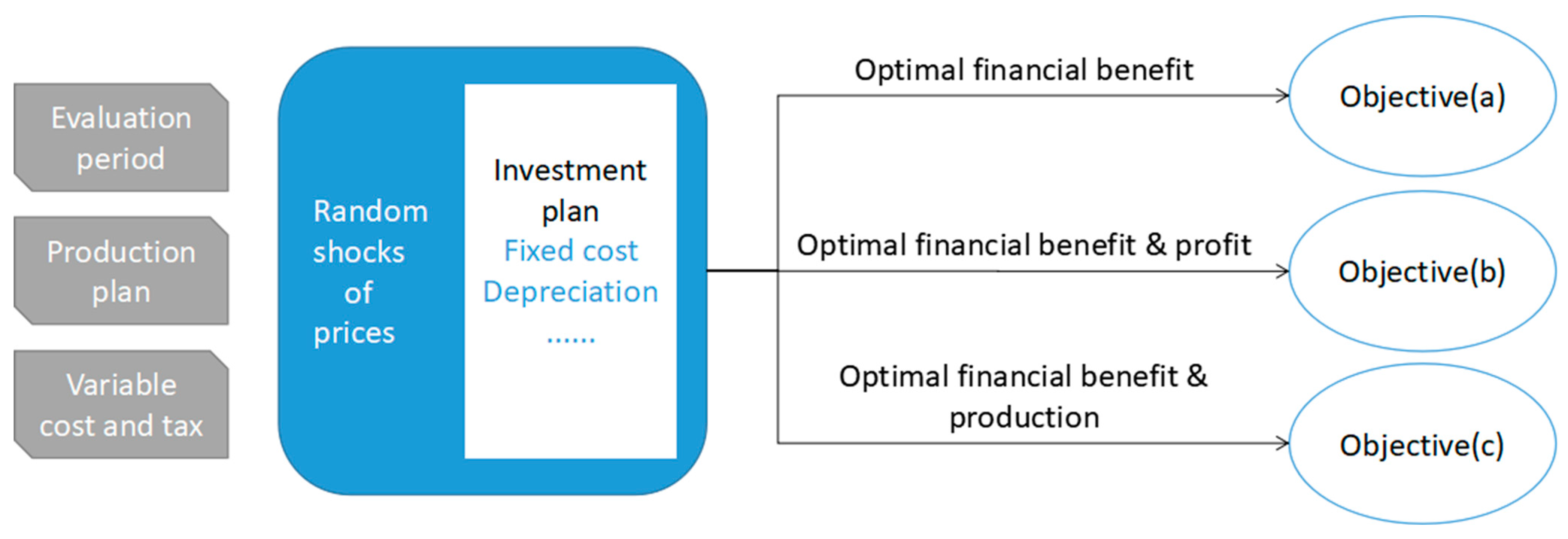
3.1. Environment
- Technical risk shock
- 2.
- Economic risk shock
- 3.
- Enterprise decision optimization
- (a)
- The project will achieve maximum financial gain.
- (b)
- The project will achieve an optimal balance between financial income and net profit.
- (c)
- The project will achieve an optimal balance between financial returns and production.
3.2. Economic Evaluation Model
3.2.1. Economic Evaluation Model of Gas Well
- Economically recoverable reserve of gas well
- 2.
- Production decline model of gas well
- 3.
- Variable cost of gas well
- 4.
- Fixed cost of gas wells
- 5.
- Depreciation of gas well
3.2.2. Natural Gas Price Forecast Model
3.2.3. Economic Evaluation Model of Gas Block
- Production, cost and depreciation
- 2.
- Price and tax
- 3.
- Income and profit
- 4.
- Financial net present value
4. Simulation Result and Discussion
4.1. Setting
4.1.1. Economic Evaluation Model
- Literature Calibration
- 2.
- Parameter setting

| Symbols | Value | Description |
|---|---|---|
| 300 | total months for 25 years, month | |
| 27 | workdays | |
| 30 | total number of gas wells | |
| (1, 8) | the mean economically recoverable reserve of all wells, 104 m3 | |
| (36, 84) | the mean stable production period of all wells, month | |
| (0.005, 0.03) | initial decline rate in Arps model | |
| (0, 1) | decline exponent in Arps model | |
| (0.1, 0.7) | unit variable cost of this block, CNY per m3 | |
| (0.5, 1.2) | mean definite fixed cost for all wells, CNY 108 | |
| 0.17 | composite tax rate of natural gas, % | |
| 0.08 | standard discount rate, % |
| Symbols | Value | Description |
|---|---|---|
| (1, 2) | expected equilibrium price | |
| 1.2 | actual ex-factory price | |
| 0 | Brownian motion | |
| 1/12 | time interval, per month | |
| N (0, 1) | normalization |
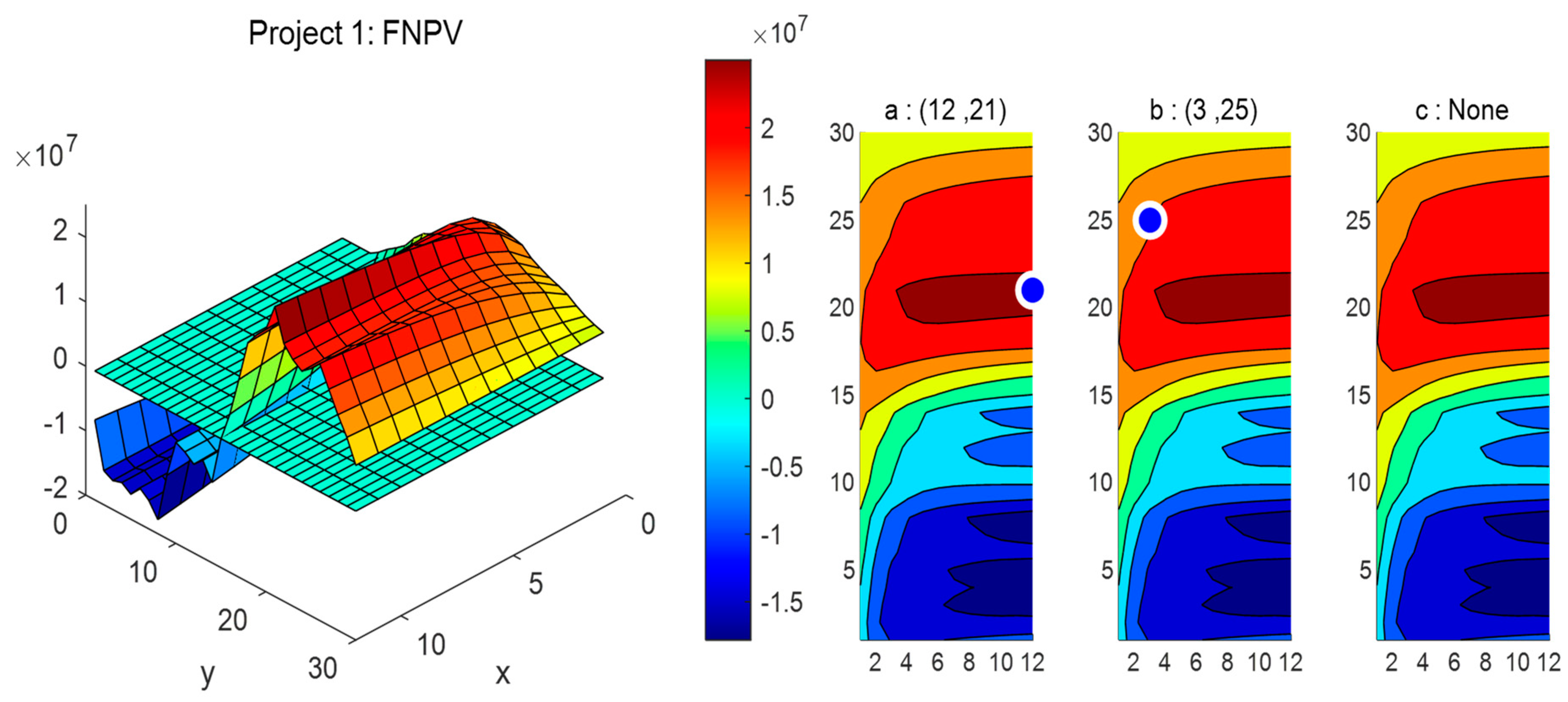
4.1.2. Decision Optimizing
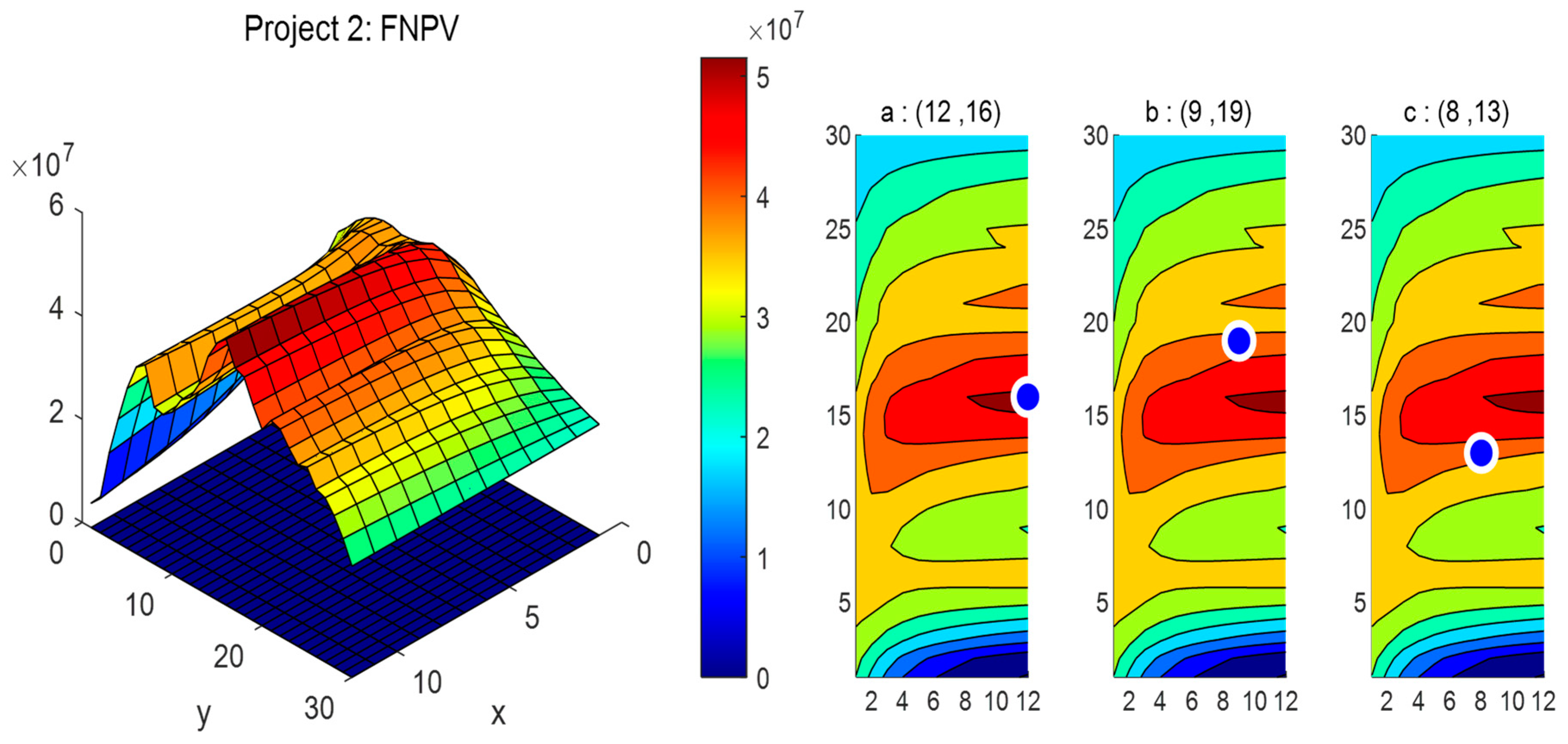
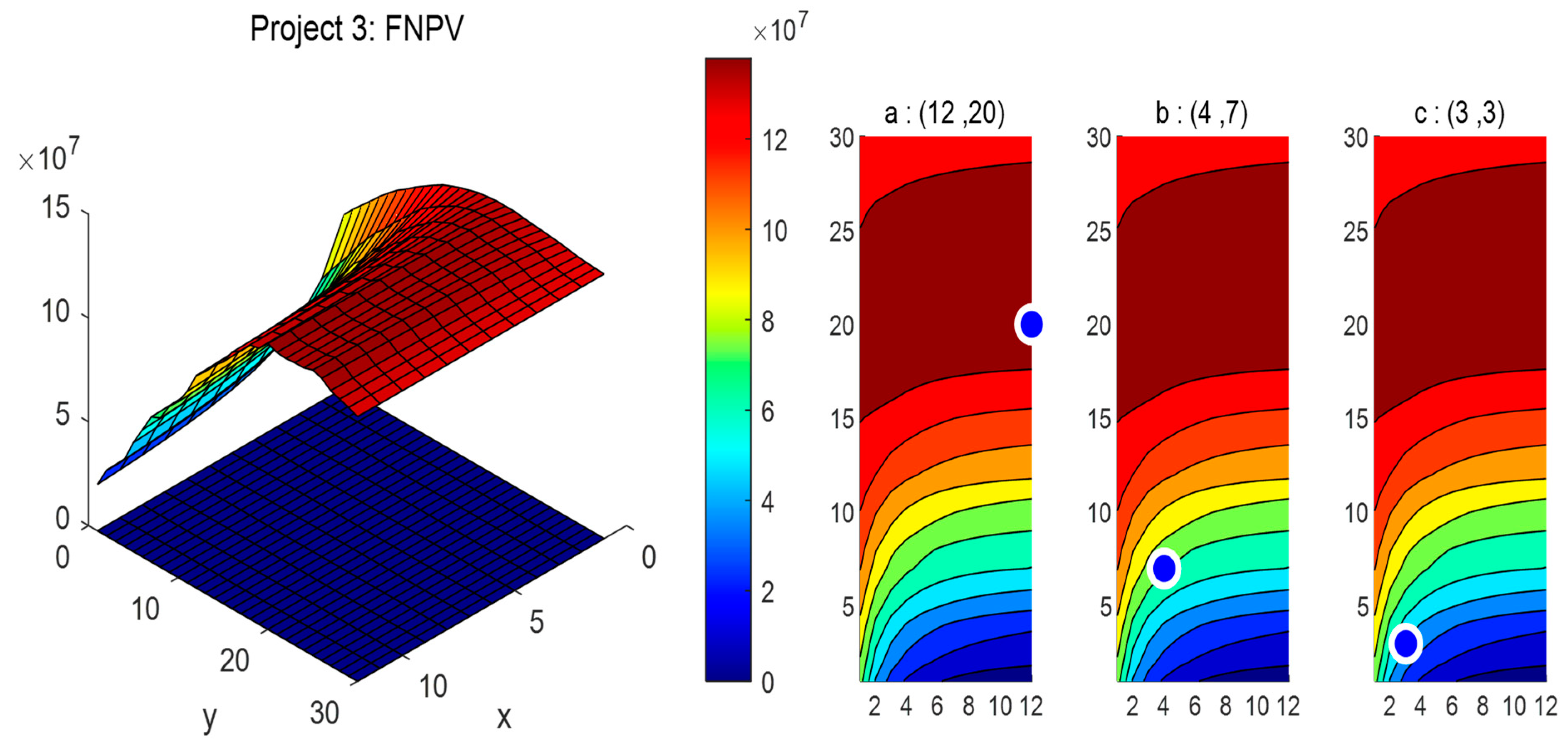
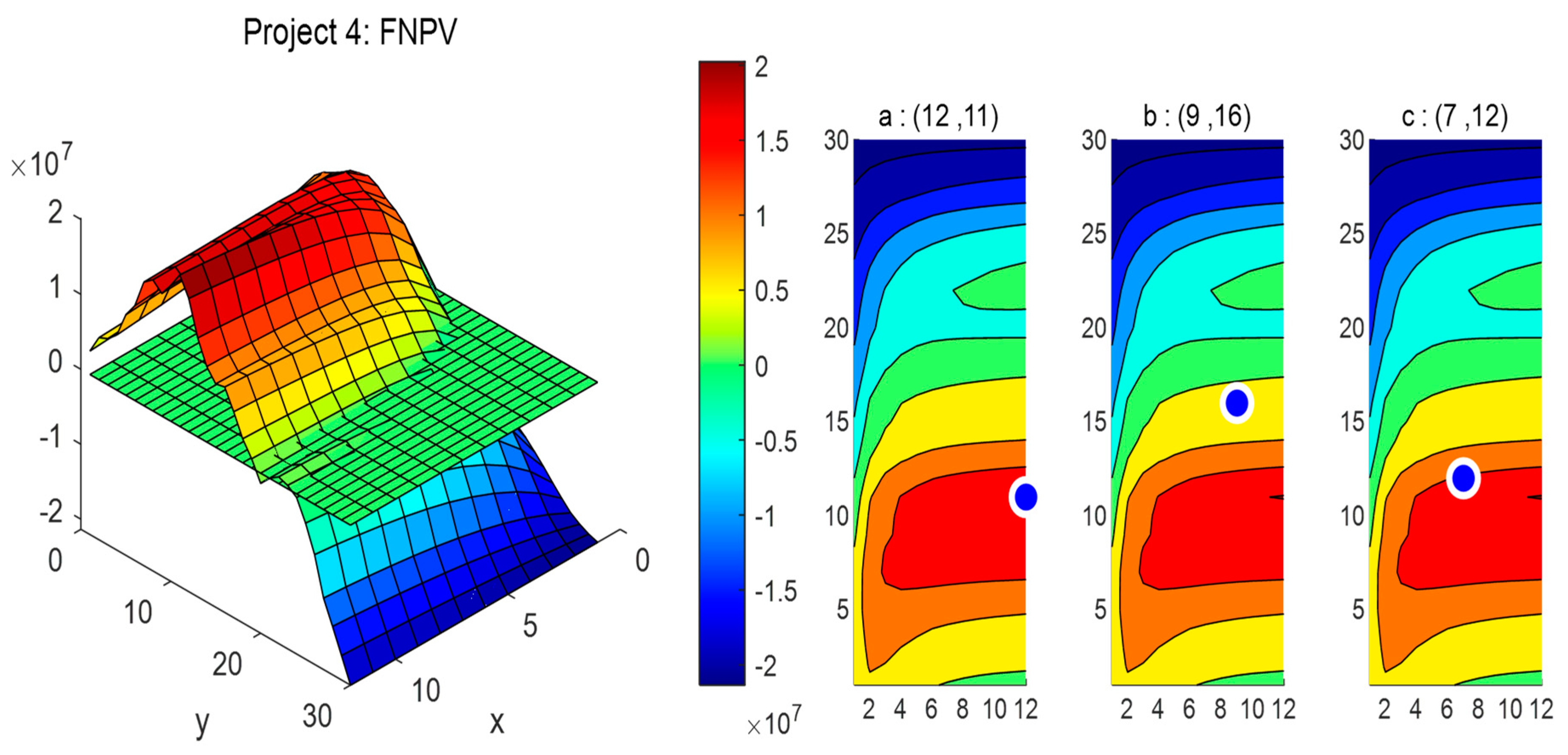
- (a)
- Positive FNPV, which is the largest among all scenarios.
- (b)
- Positive FNPV, and the net profit is greater than and closest to the average of all scenarios.
- (c)
- Positive FNPV, with yield greater than and closest to the average of all scenarios.
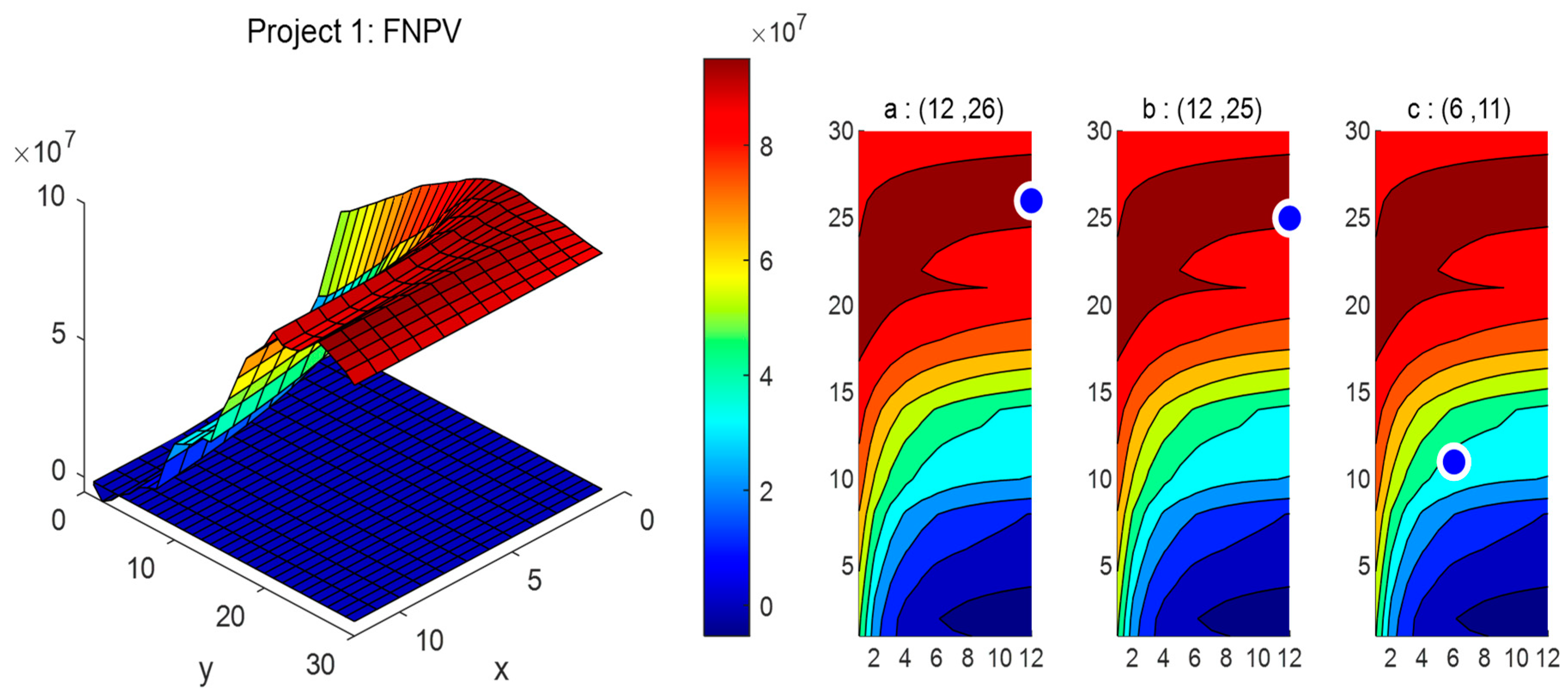
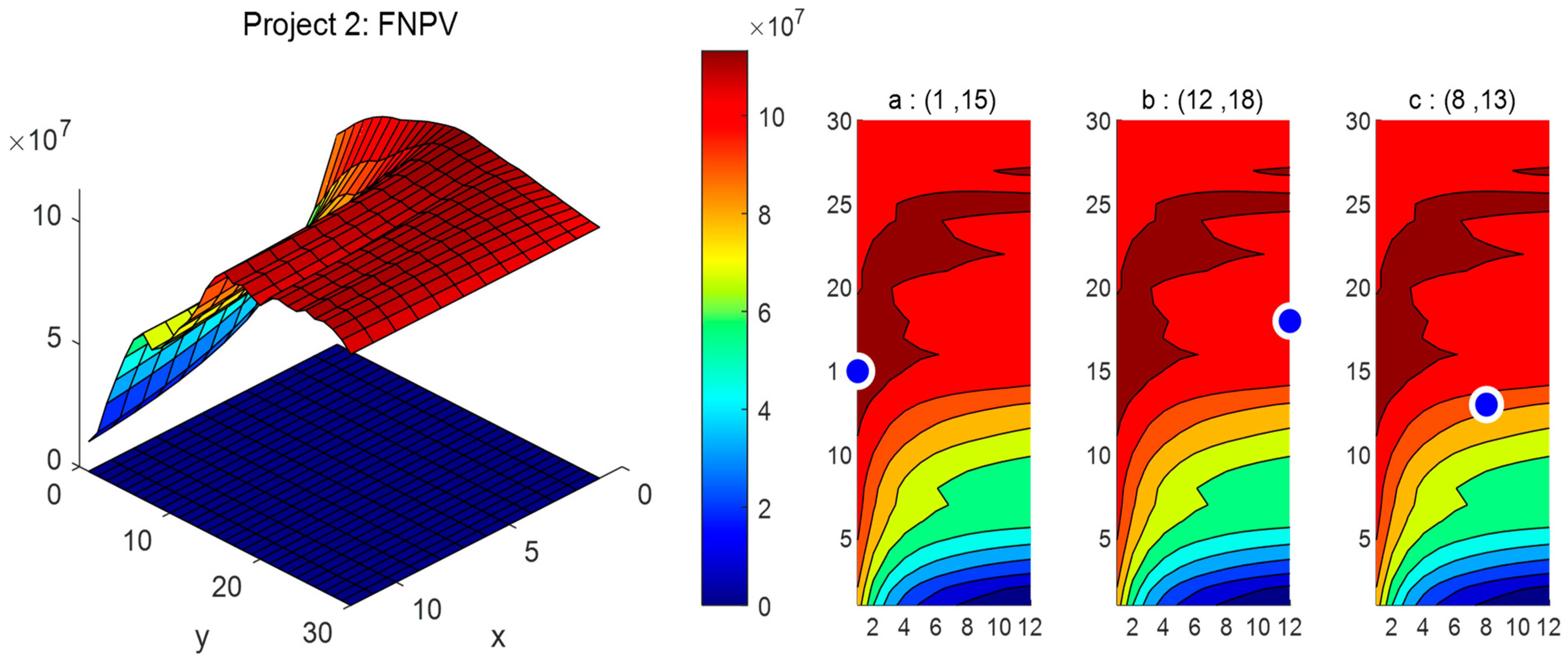
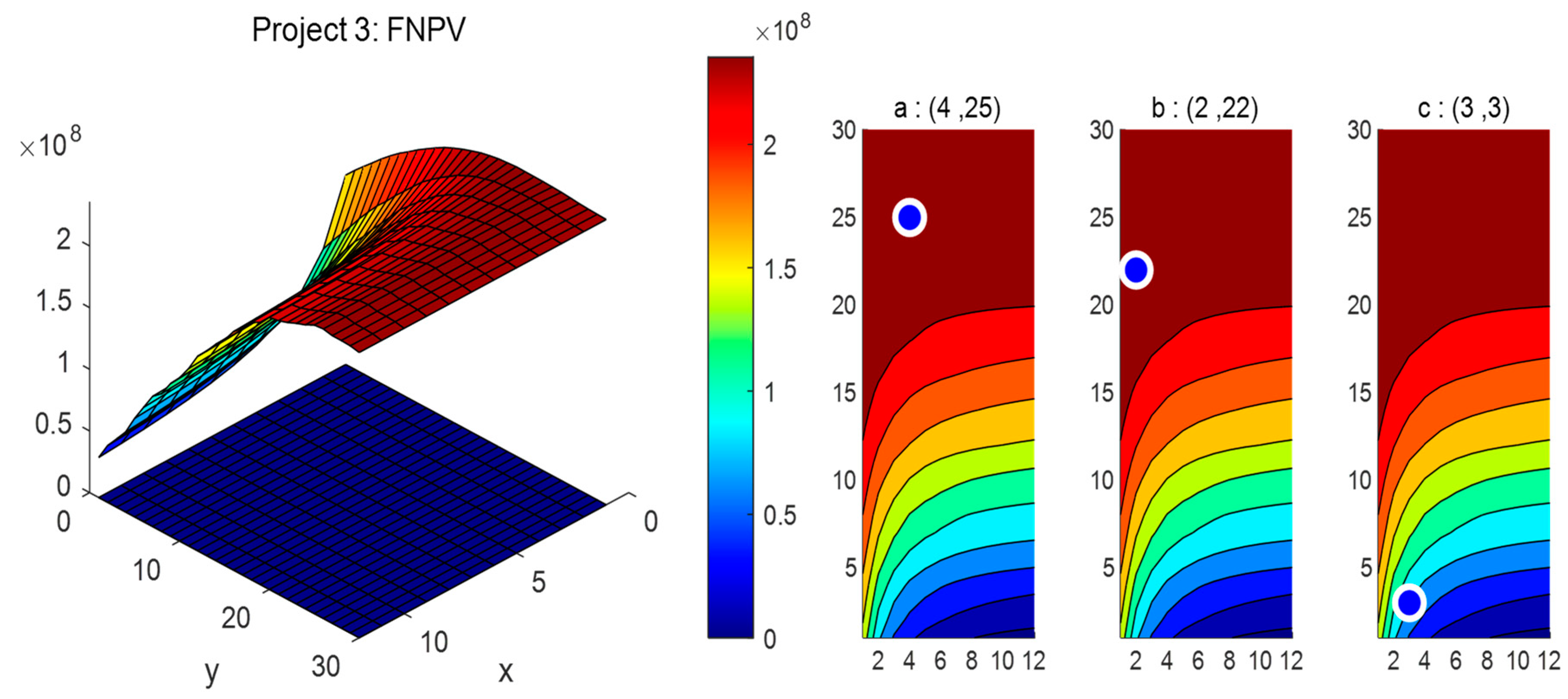
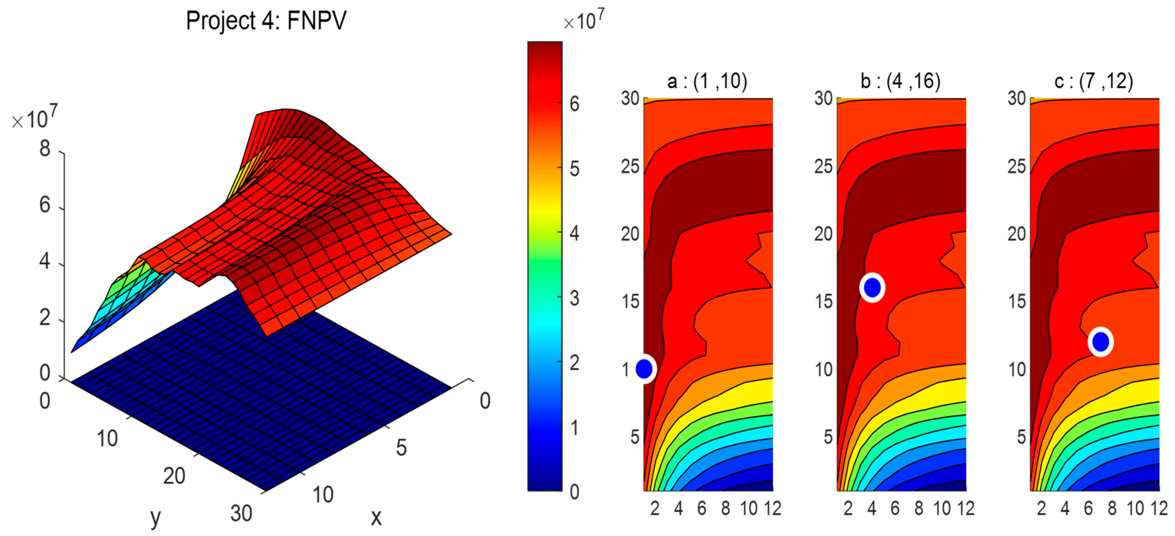
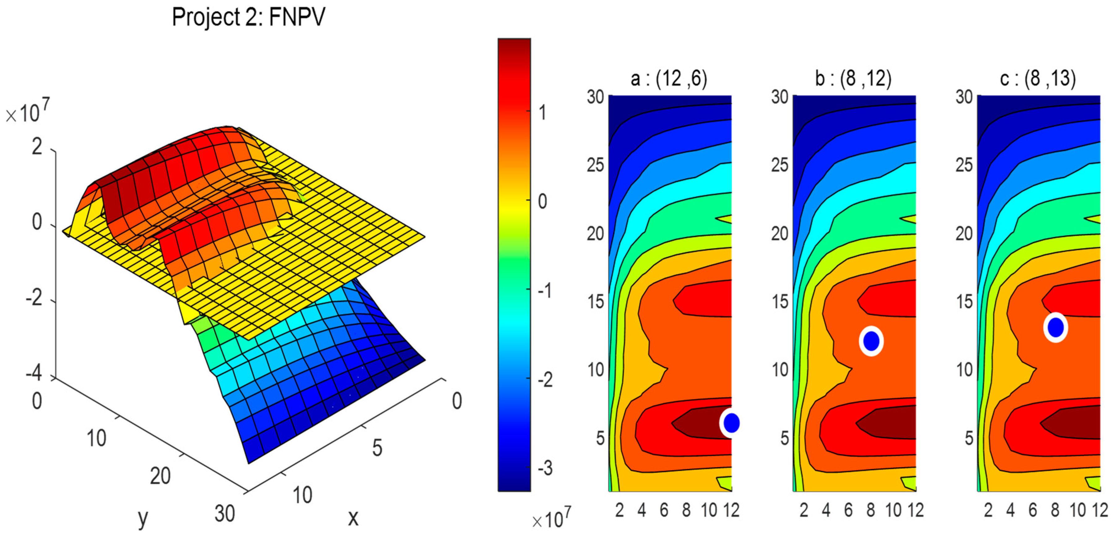
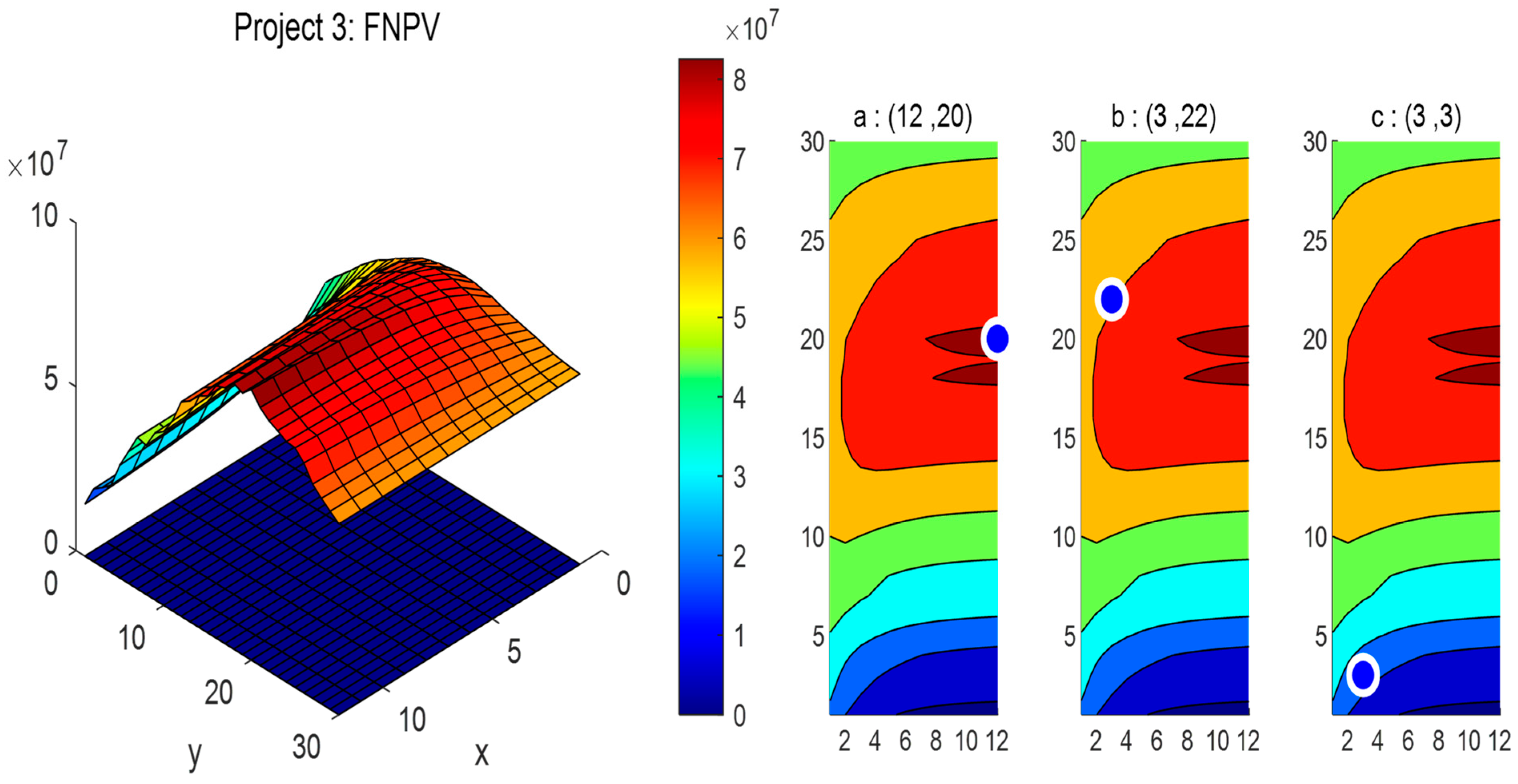
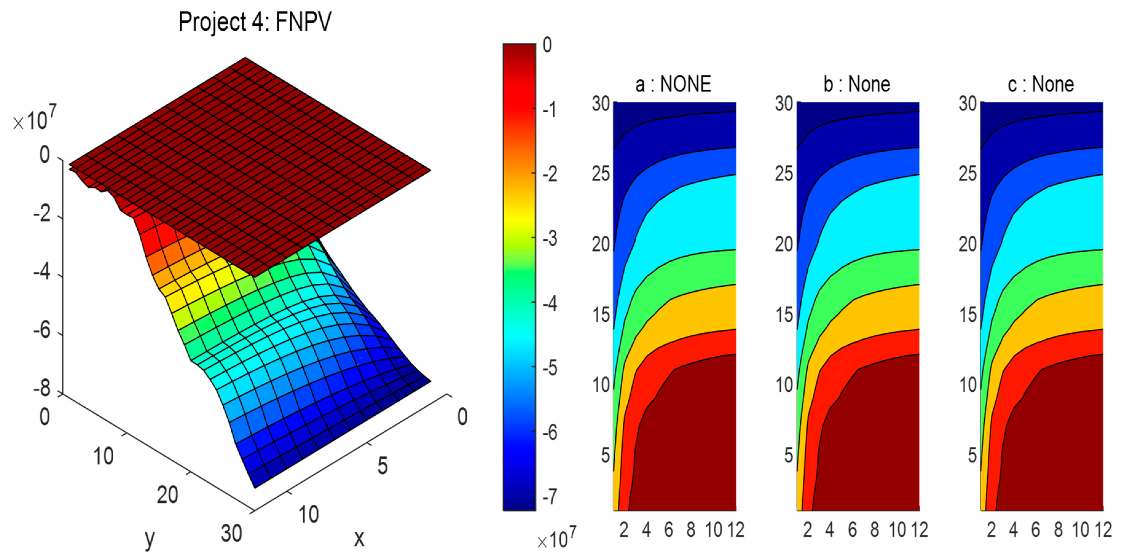
4.2. Result and Disscusion
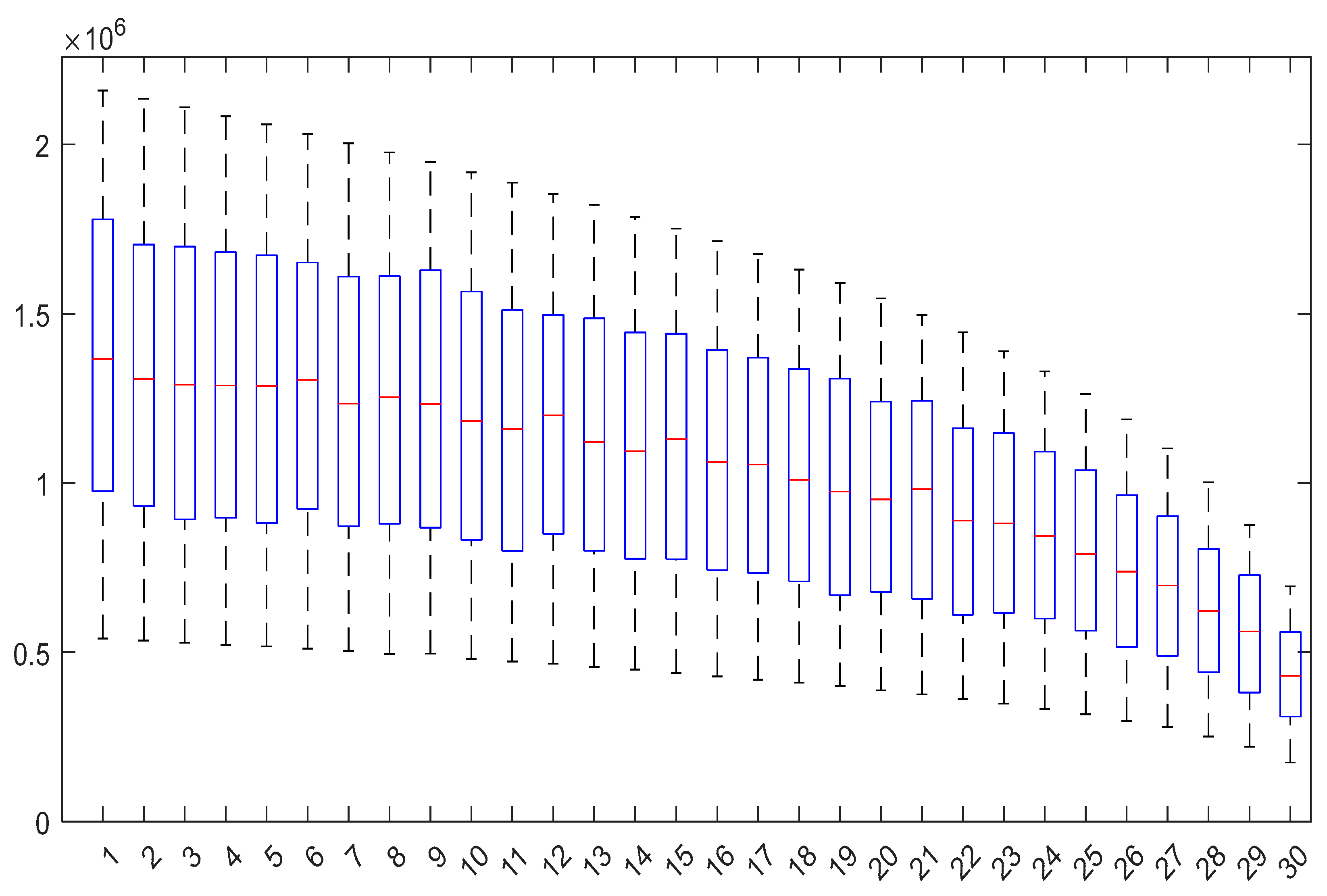
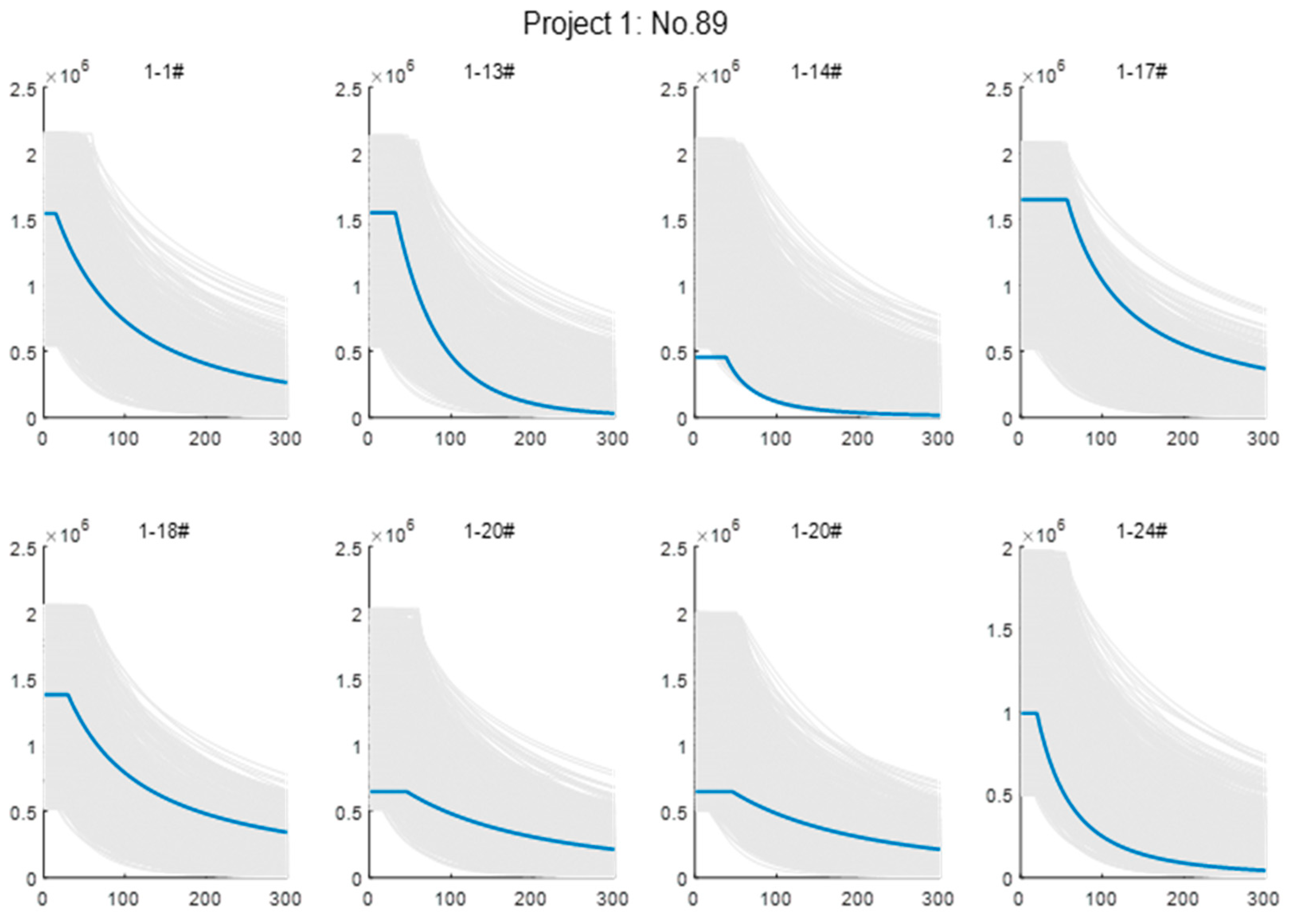
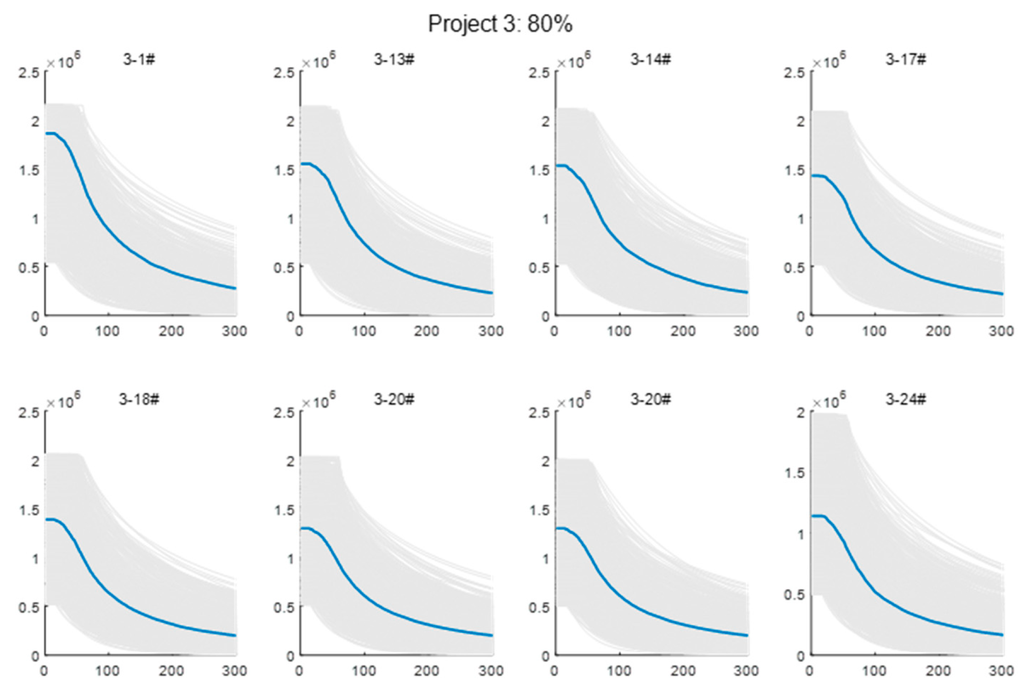
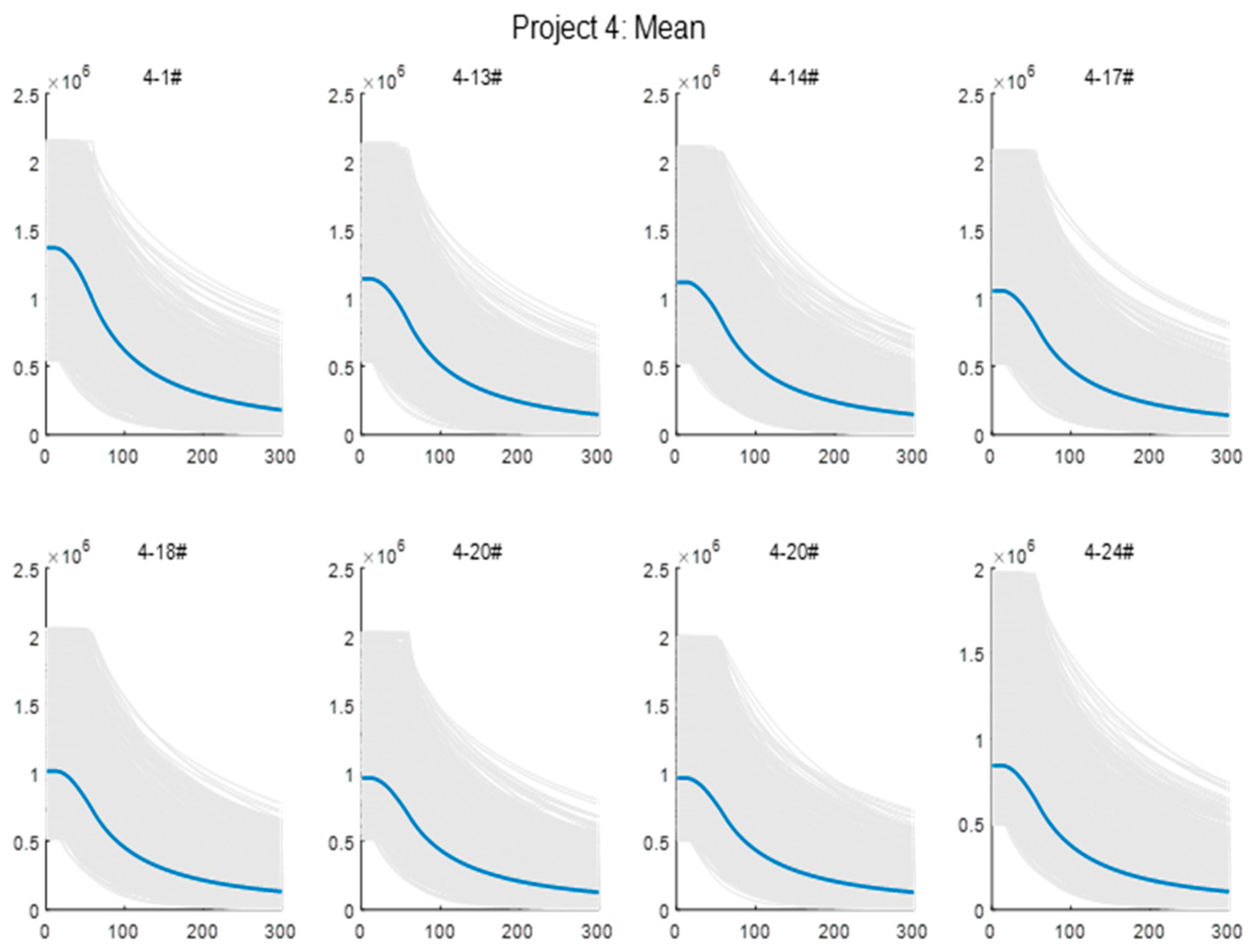
4.2.1. Production Plan
- Initial Production
- 2.
- Single well production decline simulation considering stable production period
4.2.2. The Evaluation of Investment Plan
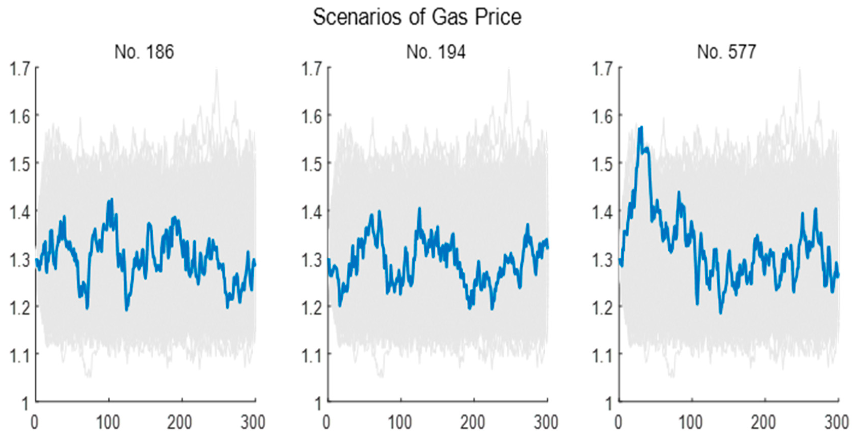
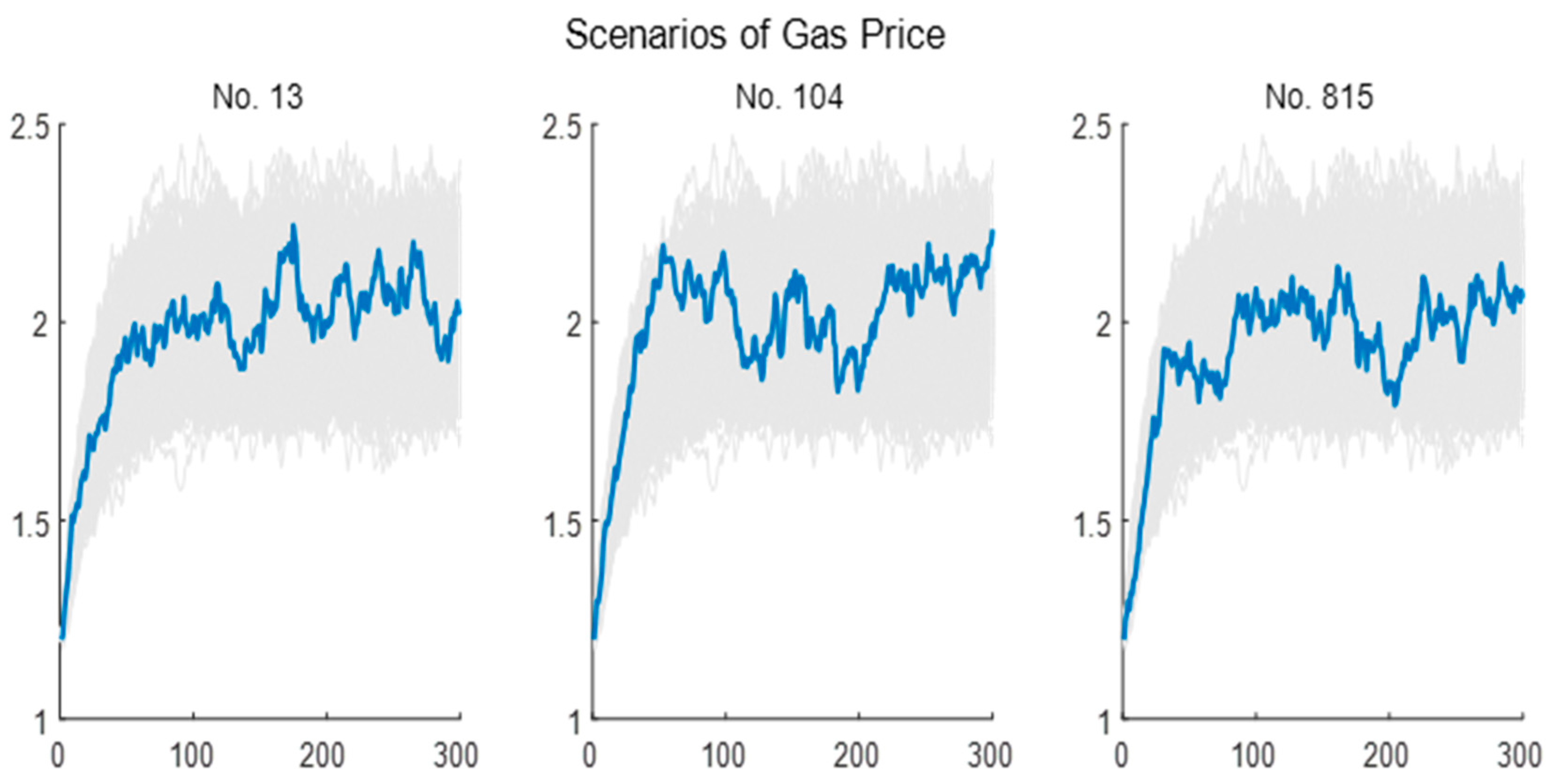
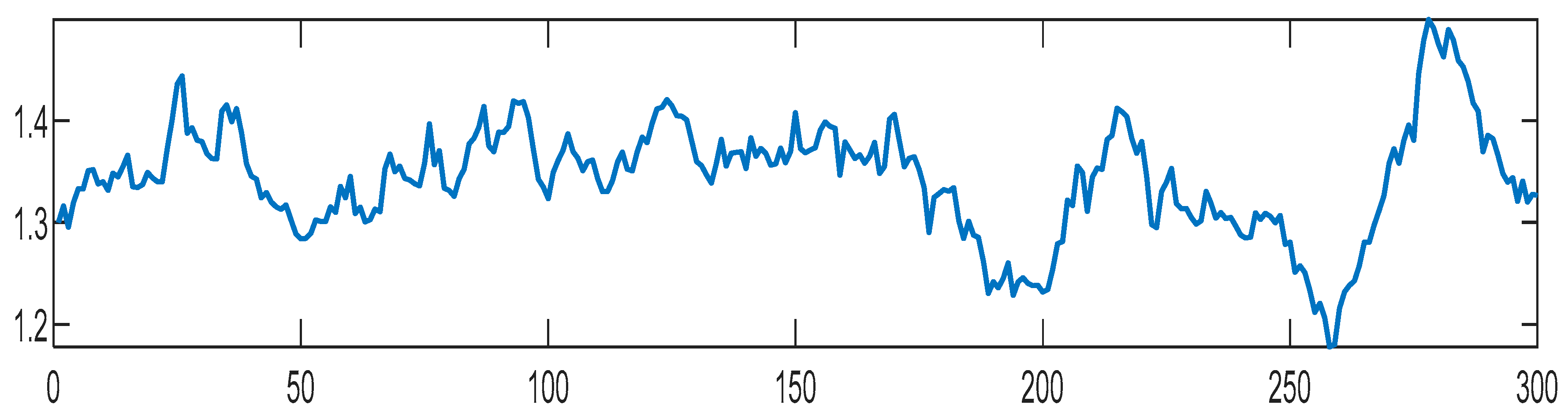
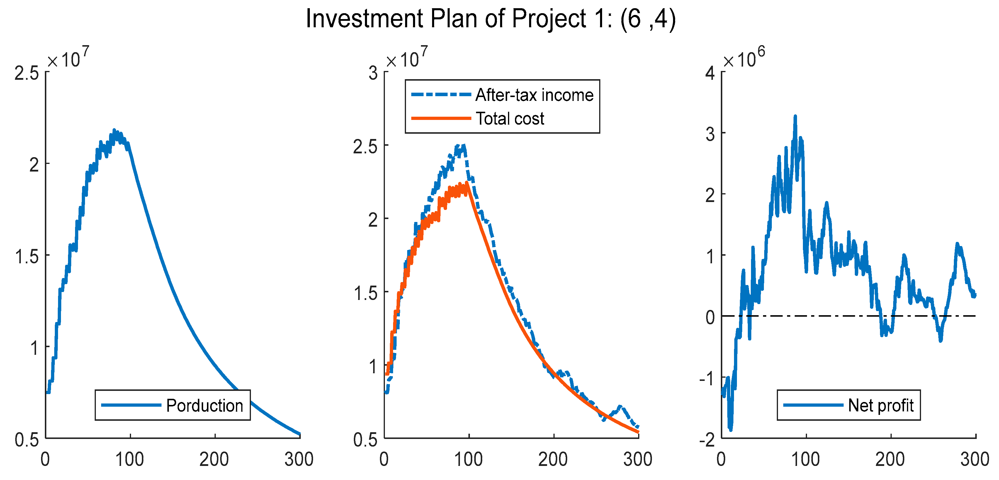
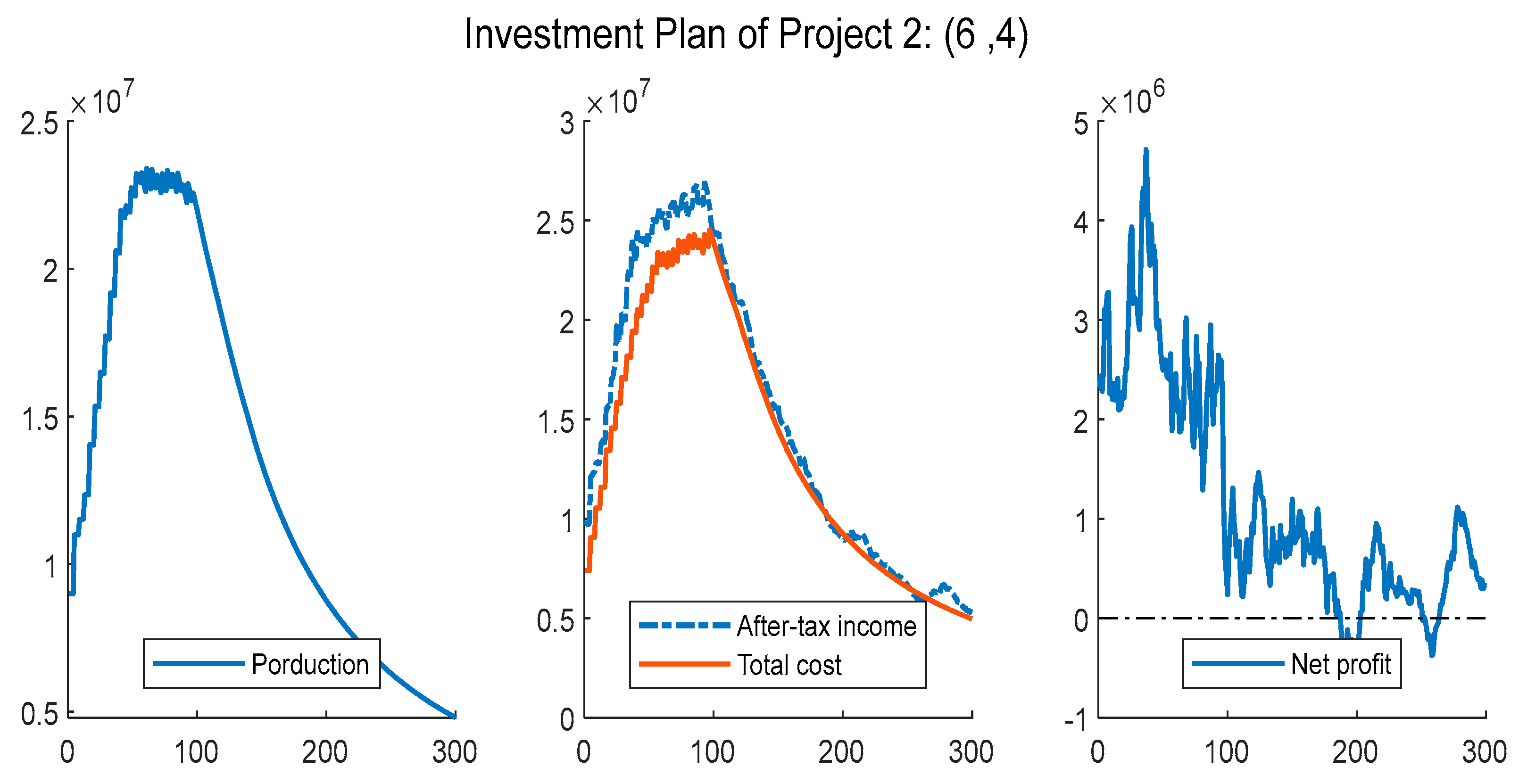
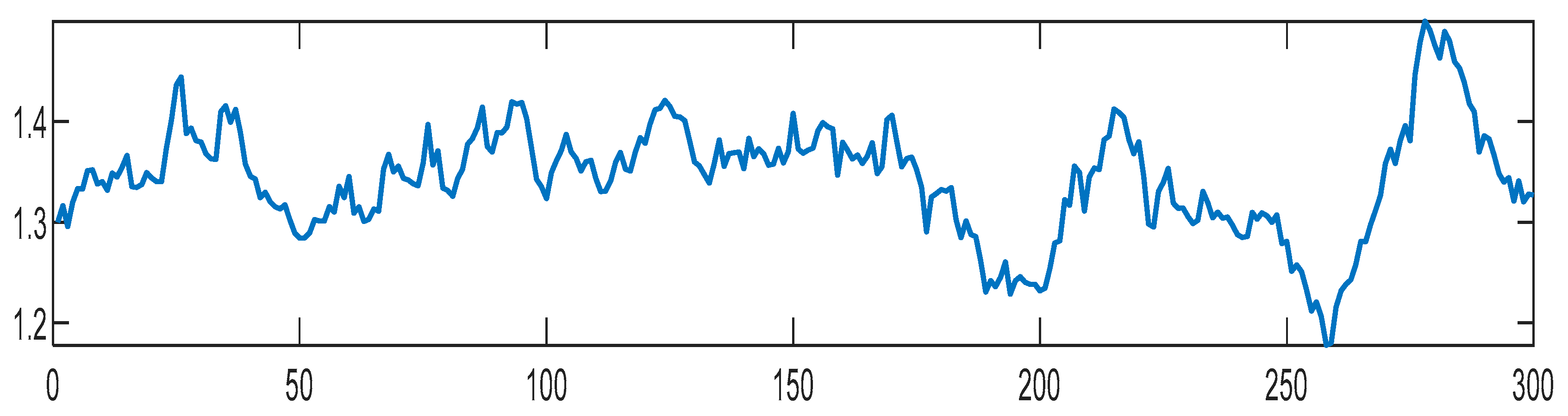
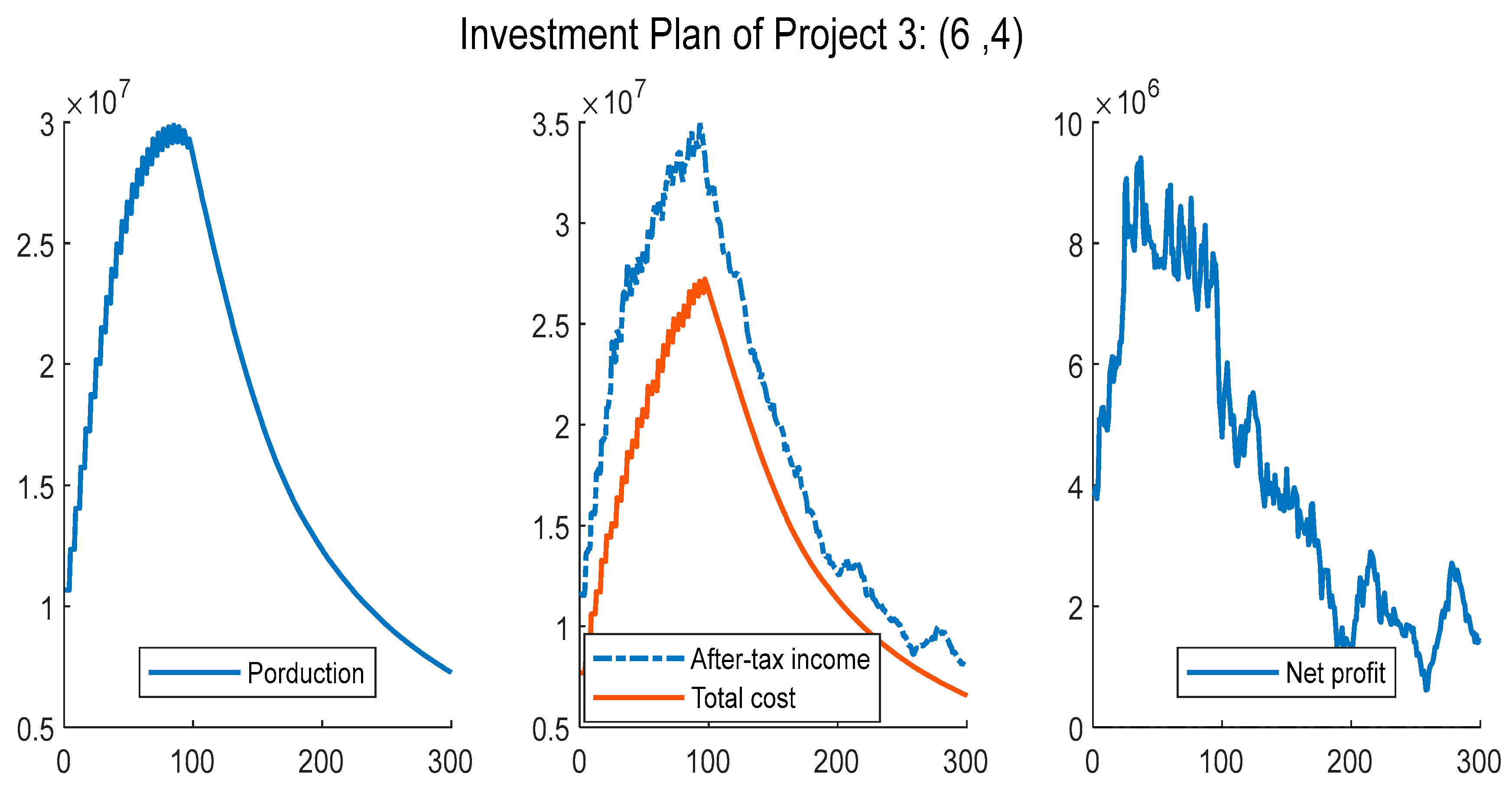
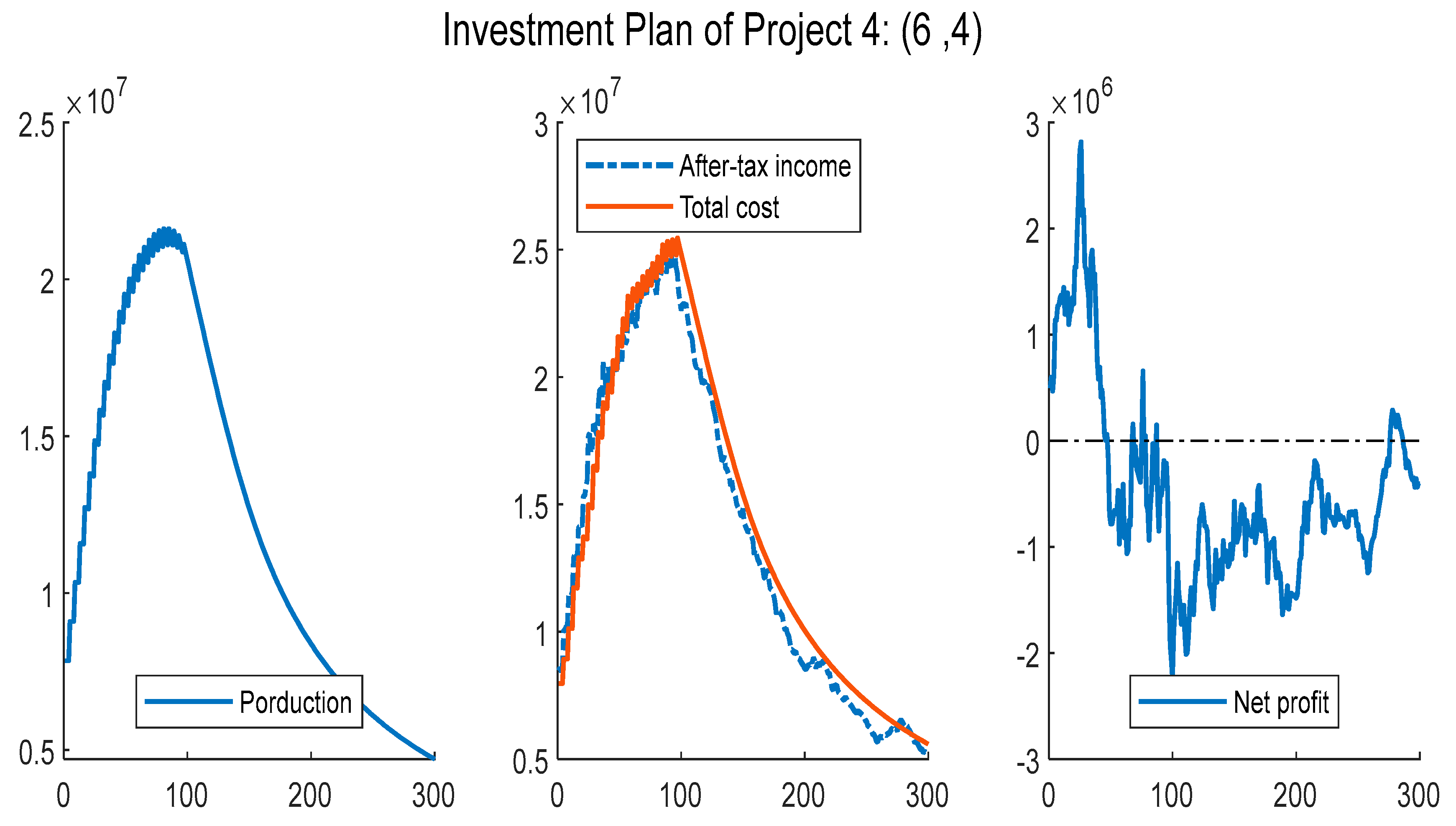
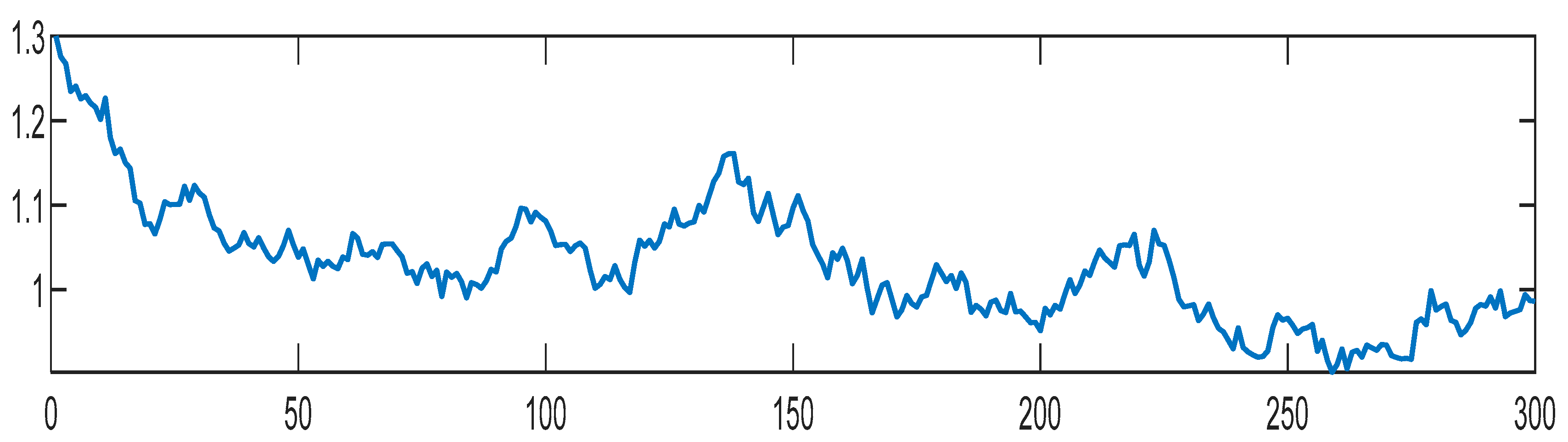
- Scenarios of Gas Prices
- 2.
- Static analysis
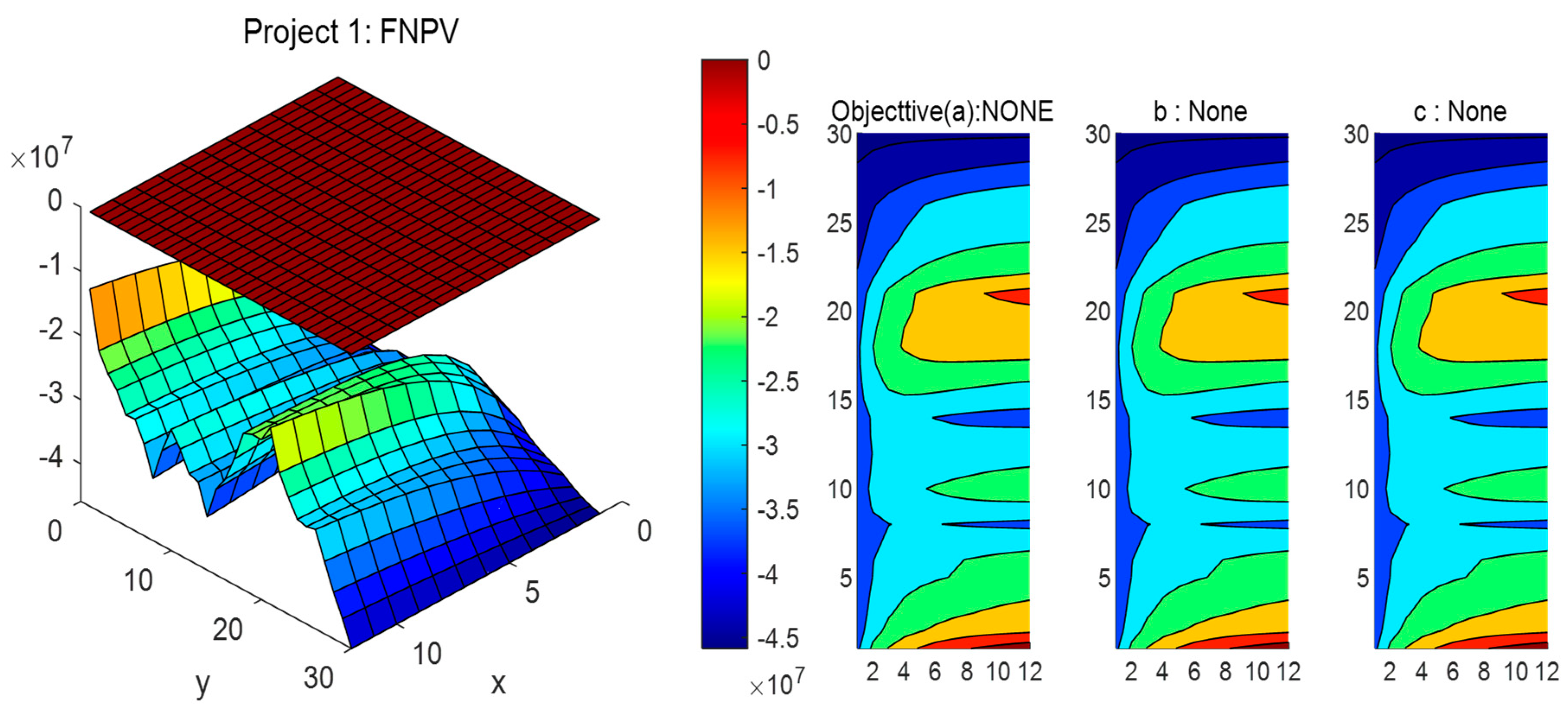
4.2.3. Optimizing
- Constant long-term mean value
- 2.
- Rising long-term mean value
5. Conclusions
Author Contributions
Funding
Data Availability Statement
Conflicts of Interest
Appendix A
- Static analysis for evaluation of investment plan


- 2.
- Decision optimization at long-term mean decline


References
- BP. BP Statistical Review of World Energy 2021 China. Available online: https://www.bp.com.cn/content/dam/bp/country-sites/zh_cn/china/home/reports/statistical-review-of-world-energy/2021/Statistical-Review-of-World-Energy-2021-China.pdf (accessed on 1 February 2023).
- NDRC. China’s Natural Gas Output up 6.7 Pct in First Two Months. Available online: https://www.ndrc.gov.cn/fgsj/tjsj/jjyx/mdyqy/202211/t20221130_1342979.html (accessed on 1 February 2023).
- NDRC. China’s National Natural Gas Operation Express in October 2022. Available online: https://en.ndrc.gov.cn/netcoo/achievements/202203/t20220322_1320514.html (accessed on 1 February 2023).
- Carvalho, A.; Riquito, M.; Ferreira, V. Sociotechnical imaginaries of energy transition: The case of the Portuguese Roadmap for Carbon Neutrality 2050. Energy Rep. 2022, 8, 2413–2423. [Google Scholar] [CrossRef]
- Wang, Z.; Kong, Y.; Li, W. Review on the development of China’s natural gas industry in the background of “carbon neutrality”. Nat. Gas Ind. B 2022, 9, 132–140. [Google Scholar] [CrossRef]
- Bouacida, I.; Wachsmuth, J.; Eichhammer, W. Impacts of greenhouse gas neutrality strategies on gas infrastructure and costs: Implications from case studies based on French and German GHG-neutral scenarios. Energy Strategy Rev. 2022, 44, 100908. [Google Scholar] [CrossRef]
- Xu, G.; Dong, H.; Xu, Z.; Bhattarai, N. China can reach carbon neutrality before 2050 by improving economic development quality. Energy 2022, 243, 123087. [Google Scholar] [CrossRef]
- Hafner, M.; Luciani, G. The Trading and Price Discovery for Natural Gas. In The Palgrave Handbook of International Energy Economics; Hafner, M., Luciani, G., Eds.; Springer International Publishing: Berlin/Heidelberg, Germany, 2022; pp. 377–394. [Google Scholar] [CrossRef]
- Institute of Climate Change and Sustainable Development of Tsinghua University. Investment and Cost Analysis for Implementing a Low Emission Strategy. In China’s Long-Term Low-Carbon Development Strategies and Pathways: Comprehensive Report; Springer: Singapore, 2022; pp. 213–226. [Google Scholar] [CrossRef]
- Xiao, J.; Cheng, J.; Shen, J.; Wang, X. A System Dynamics Analysis of Investment, Technology and Policy that Affect Natural Gas Exploration and Exploitation in China. Energies 2017, 10, 154. [Google Scholar] [CrossRef]
- Salygin, V.; Guliev, I.; Chernysheva, N.; Sokolova, E.; Toropova, N.; Egorova, L. Global Shale Revolution: Successes, Challenges, and Prospects. Sustainability 2019, 11, 1627. [Google Scholar] [CrossRef]
- Ishwaran, M.; King, W.; Haigh, M.; Lee, T.; Nie, S. China’s Natural Gas Resource Potential and Production Trends. In China’s Gas Development Strategies; Springer International Publishing: Berlin/Heidelberg, Germany, 2017; pp. 155–195. [Google Scholar] [CrossRef]
- Ishwaran, M.; King, W.; Haigh, M.; Lee, T.; Nie, S. International Natural Gas Supply and Quantities Available to China. In China’s Gas Development Strategies; Springer International Publishing: Berlin/Heidelberg, Germany, 2017; pp. 197–232. [Google Scholar] [CrossRef]
- Hámor, T.; Bódis, K.; Hámor-Vidó, M. The Legal Governance of Oil and Gas in Europe: An Indicator Analysis of the Implementation of the Hydrocarbons Directive. Energies 2021, 14, 6411. [Google Scholar] [CrossRef]
- McDonald-Buller, E.; McGaughey, G.; Grant, J.; Shah, T.; Kimura, Y.; Yarwood, G. Emissions and Air Quality Implications of Upstream and Midstream Oil and Gas Operations in Mexico. Atmosphere 2021, 12, 1696. [Google Scholar] [CrossRef]
- Arps, J.J. Analysis of Decline Curves. Trans. AIME 1945, 160, 228–247. [Google Scholar] [CrossRef]
- Fetkovich, M.J. Decline Curve Analysis Using Type Curves. J. Pet. Technol. 1980, 32, 1065–1077. [Google Scholar] [CrossRef]
- Kamari, A.; Mohammadi, A.H.; Lee, M.; Bahadori, A. Decline curve based models for predicting natural gas well performance. Petroleum 2017, 3, 242–248. [Google Scholar] [CrossRef]
- Bahadori, A. Analysing gas well production data using a simplified decline curve analysis method. Chem. Eng. Res. Des. 2012, 90, 541–547. [Google Scholar] [CrossRef]
- Xu, B.; Haghighi, M.; Li, X.; Cooke, D. Development of new type curves for production analysis in naturally fractured shale gas/tight gas reservoirs. J. Pet. Sci. Eng. 2013, 105, 107–115. [Google Scholar] [CrossRef]
- Panja, P.; Wood, D.A. Chapter Seven—Production decline curve analysis and reserves forecasting for conventional and unconventional gas reservoirs. In Sustainable Natural Gas Reservoir and Production Engineering; Wood, D.A., Cai, J., Eds.; Gulf Professional Publishing: Houston, TX, USA, 2022; Volume 1, pp. 183–215. [Google Scholar] [CrossRef]
- Cai, W.; Zhang, H.; Huang, Z.; Mo, X.; Zhang, K.; Liu, S. Development and Analysis of Mathematical Plunger Lift Models of the Low-Permeability Sulige Gas Field. Energies 2023, 16, 1359. [Google Scholar] [CrossRef]
- McGlade, C.; Speirs, J.; Sorrell, S. Methods of estimating shale gas resources—Comparison, evaluation and implications. Energy 2013, 59, 116–125. [Google Scholar] [CrossRef]
- Wei, M.-Q.; Duan, Y.-G.; Chen, W.; Fang, Q.-T.; Li, Z.-L.; Guo, X.-R. Blasingame production decline type curves for analysing a multi-fractured horizontal well in tight gas reservoirs. J. Cent. South Univ. 2017, 24, 394–401. [Google Scholar] [CrossRef]
- Wachtmeister, H.; Lund, L.; Aleklett, K.; Höök, M. Production Decline Curves of Tight Oil Wells in Eagle Ford Shale. Nat. Resour. Res. 2017, 26, 356–377. [Google Scholar] [CrossRef]
- Vikara, D.; Khanna, V. Application of a Deep Learning Network for Joint Prediction of Associated Fluid Production in Unconventional Hydrocarbon Development. Processes 2022, 10, 740. [Google Scholar] [CrossRef]
- Wang, S.; Yang, J.; Deng, C.; Tan, J. Discussion on production decline law of gas well in Sichuan gas field. Drill. Prod. Technol. 2001, 24, 27–29,33. [Google Scholar] [CrossRef]
- Wang, Y. Study on the Decline Rules of Gas Wells in Low Permeability Gas Reservoir in Su S Block. Unconv. Oil Gas 2019, 6, 77–80. [Google Scholar] [CrossRef]
- Shu, P.; Yang, X.; Liu, Y.; Zhao, X. Classification and evaluation of gas reservoirs in Daqing oilfield and optimization of development sequence. Pet. Geol. Oilfield Dev. Daqing 2004, 23, 57–58,80. [Google Scholar] [CrossRef]
- Tan, J. Development classification and countermeasures of major gas reservoirs in China. Nat. Gas Ind. 2008, 28, 107–110. [Google Scholar] [CrossRef]
- Gao, Z.; Li, Y.; Hu, Y.; Xiao, Y.; Liu, Y. Evaluation Research on Storage Classification of Natural Gas. Inn. Mong. Petrochem. Ind. 2008, 34, 16–17. [Google Scholar] [CrossRef]
- Zhou, J.; Li, Y.; Zhong, H. Classification and evaluation of water-producing gas Wells in low permeability gas reservoirs based on grey correlation analysis. J. Oil Gas Technol. 2011, 33, 143–145,160. [Google Scholar] [CrossRef]
- Wang, Y.; Hu, X.; Xu, X.; Zhang, J.; Ju, X.; Yuan, Z. Discussion of China’s Economic Recoverable Petroleum Reserves Assessment and Management. Pet. Sci. Technol. Forum 2022, 41, 25–33. [Google Scholar] [CrossRef]
- Guo, R.; Luo, D.; Zhao, X.; Wang, J. Integrated Evaluation Method-Based Technical and Economic Factors for International Oil Exploration Projects. Sustainability 2016, 8, 188. [Google Scholar] [CrossRef]
- Qiyou, R.; Xiangyang, H.; Qingfei, Z.; Kaipu, F.; Shiming, C.; Xiaojun, Z. Calculation of the economic recoverable reserves in the undeveloped area. Pet. Explor. Dev. 2004, 31, 77–80. [Google Scholar] [CrossRef]
- Adams, A.J.J.; Gibson, C.; Smith, R. Probabilistic Well-Time Estimation Revisited. SPE Drill. Complet. 2010, 25, 472–499. [Google Scholar] [CrossRef]
- Welkenhuysen, K.; Rupert, J.; Compernolle, T.; Ramirez, A.; Swennen, R.; Piessens, K. Considering economic and geological uncertainty in the simulation of realistic investment decisions for CO2-EOR projects in the North Sea. Appl. Energy 2017, 185, 745–761. [Google Scholar] [CrossRef]
- Liu, M.; Wang, Z.; Zhao, L.; Pan, Y.; Xiao, F. Production sharing contract: An analysis based on an oil price stochastic process. Pet. Sci. 2012, 9, 408–415. [Google Scholar] [CrossRef]
- Zhu, L.; Zhang, Z.; Fan, Y. Overseas oil investment projects under uncertainty: How to make informed decisions? J. Policy Model. 2015, 37, 742–762. [Google Scholar] [CrossRef]
- Chen, Z.; Wang, H.; Li, T.; Si, I. Demand for Storage and Import of Natural Gas in China until 2060: Simulation with a Dynamic Model. Sustainability 2021, 13, 8674. [Google Scholar] [CrossRef]
- Xiong, W.; Yan, L.; Wang, T.; Gao, Y. Substitution Effect of Natural Gas and the Energy Consumption Structure Transition in China. Sustainability 2020, 12, 7853. [Google Scholar] [CrossRef]
- Kong, Z.-Y.; Dong, X.-C.; Shao, Q.; Wan, X.; Tang, D.-L.; Liu, G.-X. The potential of domestic production and imports of oil and gas in China: An energy return on investment perspective. Pet. Sci. 2016, 13, 788–804. [Google Scholar] [CrossRef]
- Weijermars, R.; Sorek, N.; Sen, D.; Ayers, W.B. Eagle Ford Shale play economics: U.S. versus Mexico. J. Nat. Gas Sci. Eng. 2017, 38, 345–372. [Google Scholar] [CrossRef]
- Méjean, A.; Hope, C. Modelling the costs of non-conventional oil: A case study of Canadian bitumen. Energy Policy 2008, 36, 4205–4216. [Google Scholar] [CrossRef]
- Méjean, A.; Hope, C. Supplying synthetic crude oil from Canadian oil sands: A comparative study of the costs and CO2 emissions of mining and in-situ recovery. Energy Policy 2013, 60, 27–40. [Google Scholar] [CrossRef]
- Wang, D.; Li, X.; Liu, M.; Wang, Z. A simulation analysis on international petroleum contracts based on the stochastic process of oil price. Acta Pet. Sin. 2012, 33, 513–518. [Google Scholar] [CrossRef]
- Goel, V.; Grossmann, I.E. A stochastic programming approach to planning of offshore gas field developments under uncertainty in reserves. Comput. Chem. Eng. 2004, 28, 1409–1429. [Google Scholar] [CrossRef]
- Lin, J.; de Weck, O.; de Neufville, R.; Yue, H.K. Enhancing the value of offshore developments with flexible subsea tiebacks. J. Pet. Sci. Eng. 2013, 102, 73–83. [Google Scholar] [CrossRef]
- McIntosh, J. Probabilistic Modeling for Well-Construction Performance Management. J. Pet. Technol. 2004, 56, 36–39. [Google Scholar] [CrossRef]
- Rivera, N.; Meza, N.; Kim, J.; Clark, P.; Garber, R.; Fajardo, A.; Peña, V. Static and Dynamic Uncertainty Management for Probabilistic Production Forecast in Chuchupa Field, Colombia. SPE Reserv. Eval. Eng. 2007, 10, 433–439. [Google Scholar] [CrossRef]
- Khadem, M.M.R.K.; Piya, S.; Shamsuzzoha, A. Quantitative risk management in gas injection project: A case study from Oman oil and gas industry. J. Ind. Eng. Int. 2018, 14, 637–654. [Google Scholar] [CrossRef]
- Liu, H.-H.; Cui, Y.-H.; Liu, L.-L.; Jiang, Q.-F.; Yang, H. Production Decline Analysis Method for Fractured Gas Well in Sulige Tight Gas Reservoir Based on Arps Decline Model; Springer: Singapore, 2020; pp. 337–349. [Google Scholar]
- Gonzalez-Salazar, M.A.; Kirsten, T.; Prchlik, L. Review of the operational flexibility and emissions of gas- and coal-fired power plants in a future with growing renewables. Renew. Sustain. Energy Rev. 2018, 82, 1497–1513. [Google Scholar] [CrossRef]
- Solibakke, P.B. Forecasting Stochastic Volatility Characteristics for the Financial Fossil Oil Market Densities. J. Risk Financ. Manag. 2021, 14, 510. [Google Scholar] [CrossRef]
- Schmeck, M.D.; Schwerin, S. The Effect of Mean-Reverting Processes in the Pricing of Options in the Energy Market: An Arithmetic Approach. Risks 2021, 9, 100. [Google Scholar] [CrossRef]
- Lu, W.; Arrigoni, A.; Swishchuk, A.; Goutte, S. Modelling of Fuel- and Energy-Switching Prices by Mean-Reverting Processes and Their Applications to Alberta Energy Markets. Mathematics 2021, 9, 709. [Google Scholar] [CrossRef]
- Dong, H.; Liu, C. Study on the Decline Rule of Gas Well Production in Su A Block. Petrochem. Ind. Technol. 2018, 25, 23–24. [Google Scholar] [CrossRef]
- Chaisse, J.; Kirkwood, J. Chinese Puzzle: Anatomy Of The (Invisible) Belt And Road Investment Treaty1. J. Int. Econ. Law 2020, 23, 245–269. [Google Scholar] [CrossRef]
- Chaisse, J.; Olaoye, K.F. The Tired Dragon: Casting Doubts on China’s Investment Treaty Practice. Berkeley Bus. Law J. 2020, 17, 134. [Google Scholar]


Disclaimer/Publisher’s Note: The statements, opinions and data contained in all publications are solely those of the individual author(s) and contributor(s) and not of MDPI and/or the editor(s). MDPI and/or the editor(s) disclaim responsibility for any injury to people or property resulting from any ideas, methods, instructions or products referred to in the content. |
© 2023 by the authors. Licensee MDPI, Basel, Switzerland. This article is an open access article distributed under the terms and conditions of the Creative Commons Attribution (CC BY) license (https://creativecommons.org/licenses/by/4.0/).
Share and Cite
Yong, C.; Tong, M.; Yang, Z.; Zhou, J. Conventional Natural Gas Project Investment and Decision Making under Multiple Uncertainties. Energies 2023, 16, 2342. https://doi.org/10.3390/en16052342
Yong C, Tong M, Yang Z, Zhou J. Conventional Natural Gas Project Investment and Decision Making under Multiple Uncertainties. Energies. 2023; 16(5):2342. https://doi.org/10.3390/en16052342
Chicago/Turabian StyleYong, Chi, Mu Tong, Zhongyi Yang, and Jixian Zhou. 2023. "Conventional Natural Gas Project Investment and Decision Making under Multiple Uncertainties" Energies 16, no. 5: 2342. https://doi.org/10.3390/en16052342
APA StyleYong, C., Tong, M., Yang, Z., & Zhou, J. (2023). Conventional Natural Gas Project Investment and Decision Making under Multiple Uncertainties. Energies, 16(5), 2342. https://doi.org/10.3390/en16052342