Article

A Bayesian Optimization-Based LSTM Model for Wind Power Forecasting in the Adama District, Ethiopia

by
Ejigu Tefera Habtemariam
1,
Kula Kekeba
1,
María Martínez-Ballesteros
2 and
Francisco Martínez-Álvarez
3,*
1
Big Data and HPC Center of Excellence, Department of Software Engineering, Addis Ababa Science & Technology University, Addis Ababa P.O. Box 16417, Ethiopia
2
Department of Computer Science, University of Seville, ES-41012 Seville, Spain
3
Data Science & Big Data Lab, Pablo de Olavide University, ES-41013 Seville, Spain
*
Author to whom correspondence should be addressed.
Energies 2023, 16(5), 2317; https://doi.org/10.3390/en16052317
Submission received: 30 November 2022 / Revised: 8 February 2023 / Accepted: 20 February 2023 / Published: 28 February 2023

Abstract

:
Renewable energies, such as solar and wind power, have become promising sources of energy to address the increase in greenhouse gases caused by the use of fossil fuels and to resolve the current energy crisis. Integrating wind energy into a large-scale electric grid presents a significant challenge due to the high intermittency and nonlinear behavior of wind power. Accurate wind power forecasting is essential for safe and efficient integration into the grid system. Many prediction models have been developed to predict the uncertain and nonlinear time series of wind power, but most neglect the use of Bayesian optimization to optimize the hyperparameters while training deep learning algorithms. The efficiency of grid search strategies decreases as the number of hyperparameters increases, and computation time complexity becomes an issue. This paper presents a robust and optimized long-short term memory network for forecasting wind power generation in the day ahead in the context of Ethiopia’s renewable energy sector. The proposal uses Bayesian optimization to find the best hyperparameter combination in a reasonable computation time. The results indicate that tuning hyperparameters using this metaheuristic prior to building deep learning models significantly improves the predictive performances of the models. The proposed models were evaluated using MAE, RMSE, and MAPE metrics, and outperformed both the baseline models and the optimized gated recurrent unit architecture.

1. Introduction

Nowadays, reliable and sufficient energy is essential for human comfort. With the growing population and increasing energy-intensive industries, the demand for energy continues to rise. Renewable energy sources such as solar, geothermal, and wind energy have gained significant attention globally for their environmental benefits and contributions to the green economy [1].
Generating energy from renewable sources has become a promising solution to support sustainable economic growth and provide a healthier world for future generations [1,2]. Wind energy, in particular, is abundant and renewable, and its growth has the potential to reduce pollutant gas emissions from the use of fossil fuels [3,4]. The number and energy generation capacity of wind generation plants have increased annually as countries place a greater emphasis on renewable energy sources [5]. According to the World Wind Energy Association (WWEA), wind energy generation capacity has reached 650.8 GW globally. Ethiopia, in Eastern Africa, has the largest share of abundant renewable energy resources, including hydroelectric power, but has yet to fully tap into this potential. The potential for wind energy in Ethiopia is estimated to be about 1350 GW, with an annual installed capacity of approximately 1676 GW [6].
However, the integration of wind energy with a large-scale electric grid presents a major challenge due to the highly intermittent and nonlinear nature of wind power. Additionally, wind power generation is greatly impacted by complex atmospheric factors such as wind speed, temperature, and air pressure, which can affect wind power generation and grid operation.
To address this, accurate wind power forecasting is crucial for safely connecting wind power to the grid system and ensuring efficient grid operation [7]. Accurate forecasting of wind power generation helps keep the energy supply and demand in the grid system stable and is useful for appropriate wind farm site selection and making informed investment decisions [8]. However, the highly variable and intermittent behavior of wind power due to complex atmospheric variables makes wind power forecasting a difficult task.
In recent years, the generation of time series data from sources such as sensors and smart meters has led to the availability of large volumes of data. Time series is a sequence of observations taken at defined time intervals, which could be hourly, daily, weekly, monthly, or yearly. Time series forecasting has been widely studied in many application areas, including finance, environment, energy, and climatology. Similarly, wind power forecasting depends on uncertain wind power time series data, and accurate wind power forecasting is essential for the planning and reliable execution of power systems to ensure a continuous supply [9].
Deep learning algorithms have become popular in various research fields, such as health care, natural language processing, time series forecasting [10,11], computer vision, and image recognition [12], due to their flexible structure and effective feature learning abilities.
In the energy sector, deep learning algorithms have demonstrated exceptional performance in energy consumption and wind power forecasting. They effectively capture nonlinear time series and high-variation data, resulting in higher prediction accuracy for solar and wind energy compared to conventional methods [13,14,15]. Long short-term memory (LSTM) and gated recurrent unit (GRU) are two widely used deep learning algorithms in the field of wind power forecasting, energy consumption forecasting [16], peak load forecasting, and fault identification [13].
Hyperparameter tuning is a critical aspect of deep learning and machine learning algorithms. Hyperparameters are configurable parameters that can be adjusted to achieve optimal model performance [17]. They determine the parameters of the model during training and have a significant impact on its predictive performance [18,19]. However, manual hyperparameter tuning can be difficult and the results may not be consistent [12,20]. Automatic optimization techniques, such as grid and random search, have drawbacks, including time-consuming for larger parameter sets and a lack of optimal discovery, respectively [21]. On the other hand, Bayesian optimization (BO) is an informed approach that uses a surrogate model to evaluate only the most promising models [12,22]. It computes the posterior distribution of the objective function using the Bayes theorem, allowing for fewer sampling points and faster computation time.
Furthermore, optimizing hyperparameters while training deep learning algorithms, such as LSTM and GRU significantly improves their predictive performance [19,23]. Although numerous wind power forecasting models have been proposed [24,25,26], most of them have not utilized optimization strategies to reach desired performance levels. In other words, the use of BO in combination with LSTM models (BO-LSTM) is limited in enhancing wind power forecasting. Additionally, wind power forecasts are often specific to a single location, and the complexity and variability of wind power cannot be generalized across all sites. Thus, the aim of this paper is to apply BO to develop a robust wind power prediction model using LSTM.
BO is a global optimization technique that can be used to optimize the hyperparameters of machine learning models. It uses a probabilistic model to guide the search for the global minimum by constructing a model of the objective function being optimized.
Using BO with LSTM networks offers several benefits, including more efficient discovery of the optimal hyperparameter values compared to other optimization methods, such as grid search or random search. This is particularly useful when training deep learning models, which can be expensive optimization problems.
Another advantage of BO is its ability to handle complex and multimodal objective functions, which can arise when training LSTM networks. Unlike fixed search strategies such as grid search, Bayesian optimization uses a probabilistic model to guide the search, enabling it to handle complex optimization problems.
In conclusion, the advantages of using BO with LSTM networks include increased efficiency in finding optimal hyperparameters, the ability to handle complex and multimodal objective functions, and applicability to expensive optimization problems, such as deep learning model training.
In light of the information presented, the contribution of this paper can be summarized as follows:
  • Bayesian optimization (BO) was employed to identify optimal hyperparameters, such as the number of neurons and activation function, for the purpose of enhancing wind power forecasting.
  • The BO-LSTM model proposed in this paper was evaluated using real wind power data and found to outperform baseline methods in terms of statistical error metrics.
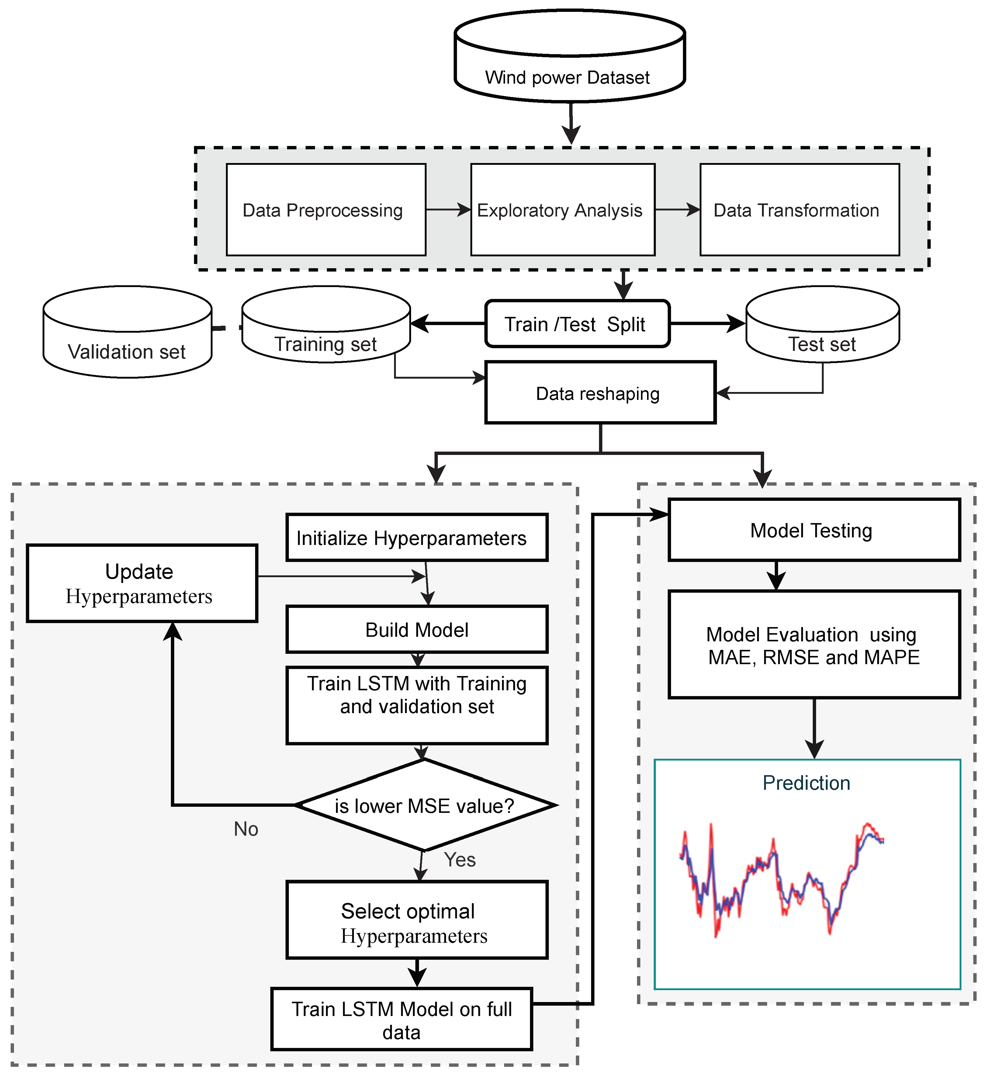
  • The paper presents a robust BO-LSTM model for day-ahead wind power forecasting, utilizing actual wind power data.
  • A wind power dataset was created for the first time in the Adama district of Ethiopia, following a comprehensive and arduous data collection process.
The rest of this paper is organized as follows. Section 2 provides a comprehensive overview of related works in the field. The methodology, including its theoretical foundations, the steps taken in data preparation, and exploratory analysis, is described in detail in Section 3. In Section 4, we present the results of our hyperparameter tuning efforts and engage in an in-depth discussion of the findings. Finally, the conclusion and suggestions for future work are presented in Section 5.

2. Related Works

This section aims to review previous studies on wind power generation forecasting that employed machine learning and deep learning models. Various methods have been utilized to predict wind power production for the purpose of making the integration of wind power with the grid system easier and more effective [27,28]. These methods can be broadly categorized into:
  • Physics-based methods: This approach predicts desired variables using real-time atmospheric variables, such as temperature, pressure, surface roughness, and obstacles. However, it is computationally intensive and may not be suitable for short-term forecasting tasks due to the high computation time and computing resources required [29,30].
  • Traditional statistical methods: Autoregressive (AR), autoregressive moving average (ARMA), and autoregressive integrated moving average (ARIMA) models are conventional statistical methods for time series forecasting, and they are effective in capturing linear mathematical relationships in time series data. However, their prediction accuracy decreases for longer forecast horizons, and they struggle to model complex seasonal patterns and exogenous variables [31,32,33]. Nevertheless, the combination of ARIMA and LSTM techniques has resulted in successful approaches in recent years [34].
  • Machine learning methods: Machine learning is a data-driven approach that maps between dependent and independent variables and is widely used for classification and prediction tasks [29]. This category includes feed-forward neural networks, support vector regression (SVR), k-nearest neighbor, fuzzy neural networks, extreme learning machines, and others. For example, Ahmed et al. [35] proposed using gradient boosting machines (GBMs) and support vector machines (SVMs) to predict wind power over medium to long-term time frames and found that the SVM model performed better with some computational run-time concerns. Another study proposed a wind turbine power generation prediction model using linear regression, k-nearest neighbor regression, and decision tree regression algorithms to predict one-minute time resolution data [36]. Shabbir et al. [37] used an SVM-based algorithm to predict wind energy production one day ahead, and they found that the proposed algorithms had better forecasting results with the lowest root mean square error (RMSE) values. However, conventional machine learning algorithms may struggle to capture temporal information effectively and produce more accurate forecasts for complex and nonlinear wind power data [38]. In [39], a method was proposed to predict power generation by exploiting wind speed data from different heights in the same area and achieved a 3.1% improvement in accuracy compared to the traditional support vector machine method. Gao proposed an approach based on grey models and machine learning for monthly wind power forecasting using data from China [40]. A hybrid model based on Laguerre polynomials and the multi-objective Runge-Kutta algorithm was proposed in [41] for wind power forecasting, and the effectiveness of the method was demonstrated using wind power data from a Chinese wind farm.
Due to the focus of this paper, this section only reviews deep learning-based strategies for wind power forecasting. Wind power is a promising energy source that can help address current environmental issues. Accurate wind power prediction is critical for the stable and optimal operation of the electric grid in power systems. Many novel models have been proposed, such as [42,43,44]. Reference [45] proposes an efficient wind power forecasting model using an LSTM network. A hybrid model of a convolutional neural network and multilayer perceptron network was developed for day-ahead wind power generation forecasting in [46]. Reference [47] introduces a hybrid method for ultra-short-term wind power prediction, taking into consideration wind power, wind direction variables, and factors from the environment and turbine disturbance. Reference [48] proposes a hybrid of convolutional neural network and informer model to predict average wind power over a period of time, effectively extracting time series features and trend information using a 2-D convolutional neural network. Reference [49] uses a sparse machine learning technique to predict next-hour wind power by combining real-time observation data with data from physical model forecast results. Reference [50] proposes a new model to forecast the electricity production of wind farms in Manisa, Turkey, using a univariate sequence-to-sequence learning model, with promising results.
The accurate prediction of wind power is important for stable and reliable power grid operation and effective integration of wind power into the electricity grid. A wavelet decomposition-based method was developed to improve the accuracy of wind power forecasting [51]. The role of wind speed forecasting in wind power generation is critical, and a hybrid model based on a GRU neural network and variation mode decomposition has been shown to effectively capture the intermittent and fluctuating behaviors of wind power [24]. LSTM is capable of accurately learning data patterns and providing results for longer temporal dependency data, such as monthly predictions [25]. A novel method based on an improved stacked GRU-RNN and multiple monitoring parameters has been used to reduce the complexity of the model, saving computational costs and requiring fewer training data [52].
RNN, a class of deep learning, is composed of sequence-based architectures that model the temporal correlation between past and current information [26]. LSTM networks, an improvement of RNN, have an internal state that can propagate data through multiple time steps, allowing them to effectively process time series data.
Putz et al. introduced a novel model based on neural expansion analysis for time series wind power forecasting in [53]. This model outperforms other statistical and classical machine learning methods and requires little to no data preprocessing. Yu et al. proposed an improved LSTM forget-gate network in [45] that uses Spectral Clustering to enhance the model’s training speed and accuracy. Mishra et al. studied a comparative analysis of five deep learning models including Deep Feed Forward, Deep Convolutional Network, RNN, Attention mechanism, and LSTM in [4]. Lin et al. used Temporal Convolutional (TCN) Network for wind power prediction in [54] and found that TCN outperforms LSTM, RNN, and GRU in terms of the data input volume, stability of error reduction, and forecast accuracy.
Prema et al. proposed a wavelet decomposition-based prediction model with LSTM learning in [55] and found that wavelet decomposition improved the capture of the intermittent variations in wind data. Duan et al. developed a hybrid forecasting model using decomposition and two deep learning models in [29] and employed variational mode decomposition to extract local features of the data. A wind power prediction model based on deep learning feature extraction and genetic algorithms was proposed in [56]. A novel genetic LSTM framework was presented in [9] to predict short-term wind power and the LSTM structure’s window size and the number of neurons were determined by genetic algorithms. In [57], a deep learning-based approach was developed for modeling and prediction of wind turbine output power and was found to be more stable and robust compared to genetic algorithms and particle swarm optimization algorithms.
Akash et al. conducted a study on long-term wind speed forecasting using machine learning and time series analysis, as reported in [58]. The results, based on evaluations of MAE and RMSE, indicated that LSTM outperformed ARIMA and the artificial neural network (ANN). In [59], a Bayesian-optimized artificial neural network was proposed to forecast hourly wind speed, with improved results over the ANN and SVM models as a result of the optimization strategy. Saini et al. in [60] proposed various machine learning algorithms to enhance wind speed forecasting and energy generation estimation. GRU performed exceptionally well compared to other machine learning approaches for the given dataset. In [28], Lin and Zhang presented a novel hybrid model for accurate wind speed prediction.

3. Materials and Methods

This section discusses the theoretical framework, exploratory analysis, and data pre-processing approaches for the proposed study. In addition, model training along with hyperparameter tuning have been addressed in this section.
After data refinement as discussed in Section 3.4, the data set was partitioned into a training set and a test set in which the training data contains the first three years (70%) and the test set contains the last year ( 30 % ) wind power data in order to keep the importance time order. As the main part of the methodology of this paper, building the LSTM model on the training set by defining hyperparameter space and fine-tuning the model is implemented by using Bayesian optimization to search for the best hyperparameters combination with minimum loss values. Based on the optimal hyperparameter configuration, the proposed wind power forecasting model was trained on the wind power dataset of the three sites (groups) and the performance of each model was evaluated on the test dataset. Meanwhile, to ensure whether the proposed BO-LSTM outperforms other algorithms or not, different baseline models were studied with each dataset. The methodology of this paper is detailed in Figure 1.

3.1. Deep Learning Architectures

RNN is a type of deep learning algorithm commonly utilized in speech recognition, emotional analysis, and text analysis. Unlike deep feed-forward neural networks (DFFNNs), RNNs incorporate feedback loops and internal connections between hidden units. These internal connections enable RNNs to effectively use past data to predict future data [61]. As a result, RNN is capable of processing sequential data and identifying both short-term and long-term dependencies. It is particularly useful for time series modeling and forecasting of data with temporal correlations. Training of RNNs typically involves back-propagation through time to learn the temporal correlations in sequence data. However, RNNs can suffer from the vanishing gradient problem, where the stability of gradient propagation across time steps decreases, leading to an inability to learn long-term dependencies between inputs and predictions [62]. This occurs when the weight updates are proportional to the gradient, but small or vanishing gradients result in minimal changes to the weight values. LSTM and GRU were developed to address the limitations of RNNs by allowing for the learning and storage of longer sequence data, and effectively handling high volatility and seasonal variation in time series data.

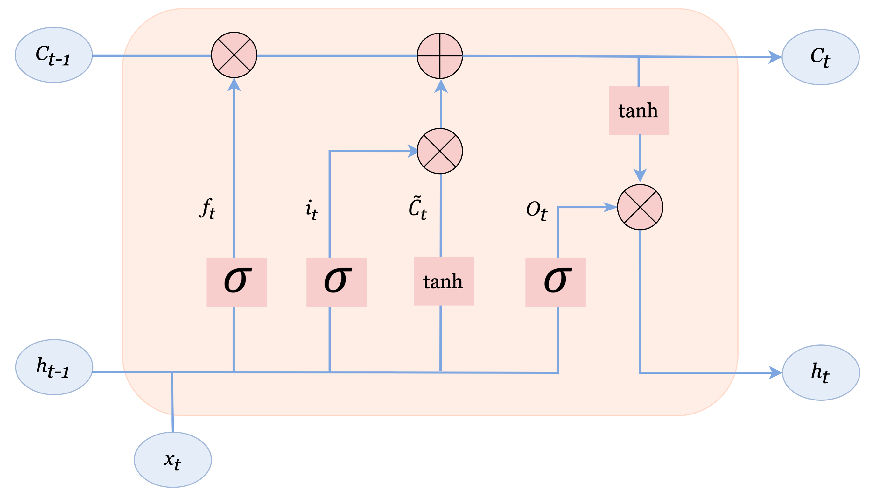
3.1.1. Long-Short Term Memory Network

LSTMs are better equipped to handle information with longer temporal dependencies and lag features in sequence data processing [63]. Unlike standard DFFNNs, which operate in a forward learning style, LSTMs have a specialized memory unit [64] to store previous operation values for use in dealing with temporally dependent data. LSTMs consist of a cell unit and gate modules, as illustrated in Figure 2 [65]. The gates include a forget gate, an input gate, and an output gate, which regulate the flow of data into and out of the cell state during processing [66]. The input gate controls updates to the memory cell from the input and the forget gate decides which information to keep and which to discard [64], while the output gate determines the information to pass to the next state. LSTMs have been widely used in time series forecasting and have achieved remarkable performance [67,68]. Their main advantage lies in their memory cell, which serves as a specialized neuron structure for storing information over long time gaps [15]. The mathematical representation of the LSTM cell can be defined in Equations (2)–(6).
f t = σ ( w f × [ h t 1 , x t ] + b f )
i t = σ ( w i × [ h t 1 , x t ] + b i )
C ˜ t = t a n h ( w c × [ h t 1 , x t ] + b c )
C t = f t C t 1 + i t C ˜ t
O t = σ ( w o × [ h t 1 , x t ] + b o )
h t = O t t a n h ( c t )
where f t , i t , and C ˜ t denote the forget gate, the input gate, and the candidate cell state, respectively; O t represents the output gate; C t and h t are the cell output at the current time t; C t 1 and h t 1 are the cell outputs at the previous time x t 1 , and x t is the input to the LSTM cell. w is the weight of neurons, and b is the bias for each weight.
The LSTM network’s ability to learn more complex tasks is due to the use of nonlinear activation functions, namely the sigmoid function σ and the hyperbolic tangent function t a n h . The sigmoid function is a nonlinear activation function that maps data to values between 0 and 1, while the hyperbolic tangent function maps data to values between −1 and 1. The sigmoid and hyperbolic tangent activation functions can be expressed mathematically in Equation (7) and Equation (8), respectively.
σ ( x ) = 1 1 + e x
t a n h ( x ) = e x e x e x + e x = 1 e 2 x 1 + e 2 x
There are several advantages of using LSTM networks for wind energy forecasting compared to other methods:
  • Handling long-term dependencies: One of the main challenges in wind energy forecasting is capturing long-term dependencies in the data. LSTMs are particularly well suited for this task because they are designed to handle long-term dependencies by selectively forgetting or retaining information from previous time steps.
  • Handling non-linear relationships: Wind energy is affected by many non-linear factors, such as temperature, humidity, and pressure. LSTMs are capable of capturing non-linear relationships in the data, making them a good choice for wind energy forecasting.
  • Handling multivariate time series: LSTMs can handle multiple inputs, making them well suited for multivariate time series data, such as wind energy data, which often includes multiple sources of information.
  • Good performance: LSTMs have shown good performance in wind energy forecasting tasks, outperforming traditional time series forecasting methods, such as ARIMA and SARIMA.
  • Robustness to noise: LSTMs are less sensitive to noise in the data compared to traditional time series methods, making them a good choice for wind energy forecasting where data quality can be a challenge.
Overall, LSTMs offer several advantages in wind energy forecasting, making them a popular choice among researchers and practitioners in the field.

3.1.2. Gated Recurrent Unit Neural Network

GRU is a newer version of LSTM and is capable of learning temporal dependencies in data to avoid the long-term dependency-learning problems of RNN [69]. Compared to LSTM, GRU has a simpler architecture with two gates, the update gate and the reset gate, as illustrated in Figure 3. In GRU, there is no cell state and the update gate combines the input and forget gates. The update gate determines what information from the previous hidden state to bring into the current state [70] and decides the amount of previous information to be memorized in the current state. The reset gate determines the aggregation of the previous information with the current input [71]. The reset gate also decides which information to discard from the previous states. The reset gate controls the capture of short-term dependencies in the sequence data, while the update gate is responsible for activating and filtering the long-term sequence data. GRU has a faster training time due to its fewer parameters compared to LSTM.
The mathematical representation of GRU operations can be defined as in Equations (9)–(12):
r t = σ W r h t 1 , x t
z t = σ W z h t 1 , x t
h t ˜ = t a n h W h r t h t 1 , x t
h t = 1 z t r t h t 1 , x t
where r t and z t are the reset and update gates, respectively, in a GRU operation. Additionally, x is the input vector, while h ˜ t and h t denote the candidate output and the output vector, respectively.

3.2. Bayesian Optimization

The performance of machine learning algorithms, especially deep learning-based predictive models, can be improved through hyperparameter optimization. Grid search and random search are the most commonly used methods for finding the optimal combination of hyperparameters to produce more accurate models. However, the efficiency of grid search decreases with the increasing size of the number of hyperparameters, and its computational time complexity is high due to the exponential increase in the number of evaluations required with each additional parameter [19]. On the other hand, random search uses a combination of randomly sampled parameters based on a statistical distribution, which can be ineffective in finding optimal hyperparameter points for some complex models [72].
Bayesian optimization (BO) is an efficient strategy for solving computationally expensive functions without a closed-form expression [73]. It builds a probability model of the objective function to determine the optimal hyperparameters in an informed manner, reducing the number of times the objective function needs to be run by choosing only the most promising set of hyperparameters. The BO approach consists of two basic components:
  • Surrogate (probabilistic) model: BO is guided by Bayes’ theorem, and in each iteration, it uses a surrogate model to approximate the objective function, which can be sampled efficiently. A Gaussian process is the most effective surrogate model for selecting the promising set of hyperparameters to be evaluated in the true objective function [74]. The surrogate model estimates the objective function, which is used to guide future sampling.
  • Acquisition function: BO uses an acquisition function [75] to determine which points in the search space should be evaluated and to provide information on the optimal value of f. The purpose of the acquisition function is to use posterior information to find the best sample point in each iteration and to propose a new sampling point to identify the most promising set of hyperparameters to be evaluated next. The acquisition function balances exploitation and exploration. Exploitation involves focusing on the search space with a higher likelihood of improving the current solution based on the current surrogate model, while exploration is the strategy of moving towards less explored regions of the search space.
BO solves problems by finding the parameters that minimize the objective function in a finite domain, with lower and upper bounds on every variable, as given by Equation (13).
x = arg min x X f ( x )
where f ( x ) represents a score that should be minimized, X is the domain of the hyperparameter values, and x is a combination of hyperparameters that produces the lowest value of the score f ( x ) .
Finally, BO can be used in conjunction with LSTMs to achieve improved performance in wind energy forecasting. Such a combination can bring several benefits, including:
  • Efficient hyperparameter tuning: BO provides a more efficient and effective way of tuning the hyperparameters of an LSTM model than traditional grid search or random search methods. It does this by intelligently selecting the next set of hyperparameters to evaluate based on the results of previous evaluations, leading to faster convergence and better results.
  • Improved model performance: By tuning the hyperparameters of an LSTM model using BO, the model can be improved to better fit the wind energy data and achieve higher accuracy in its predictions.
  • Better understanding of the model: BO can provide insights into the impact of different hyperparameters on the performance of the LSTM model, allowing for better understanding of the model and its behavior.
  • Robustness to hyperparameter selection: By using BO to select the hyperparameters, the model can be made more robust to the choice of hyperparameters, reducing the risk of poor performance due to poor hyperparameter selection.

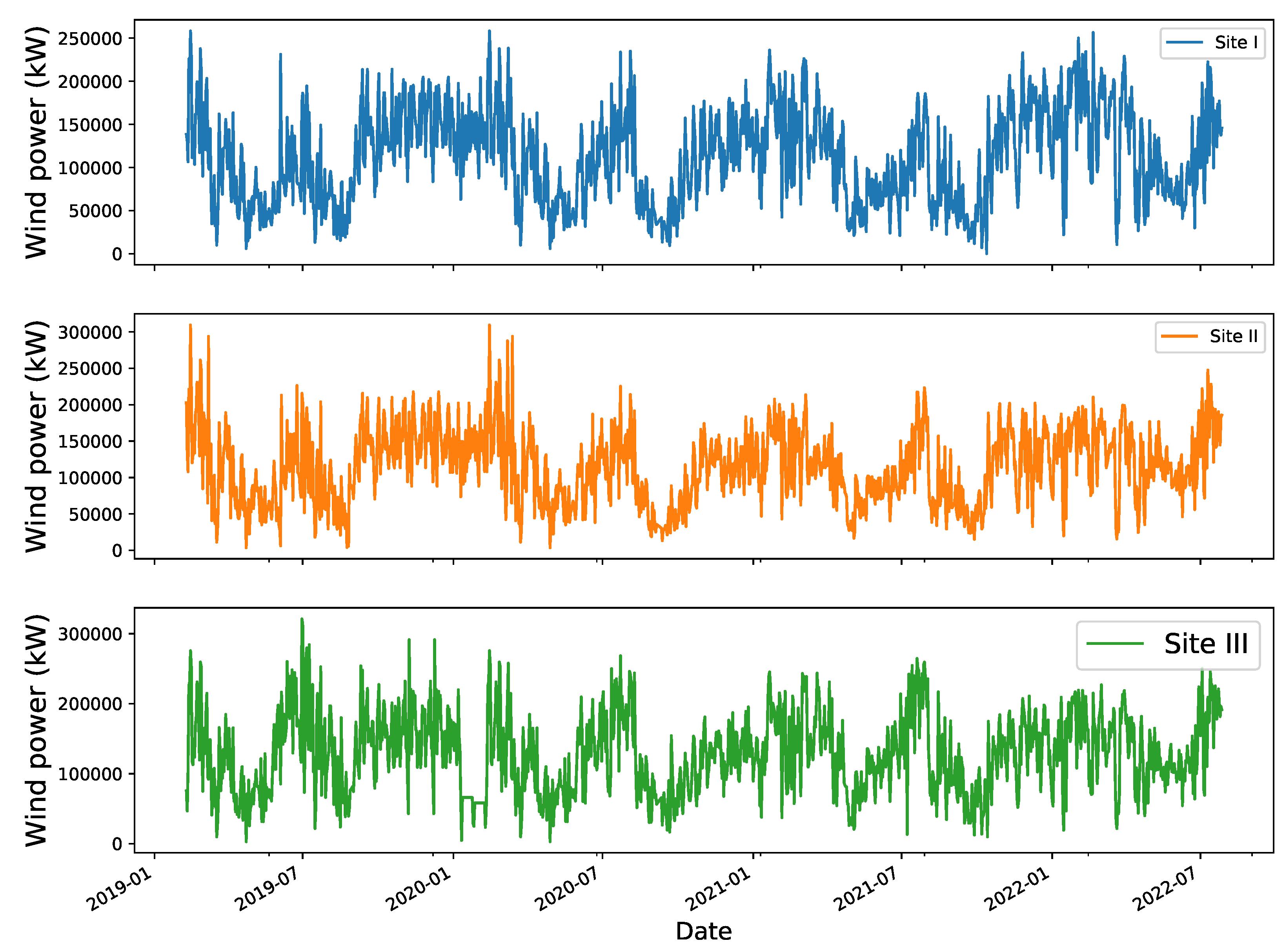
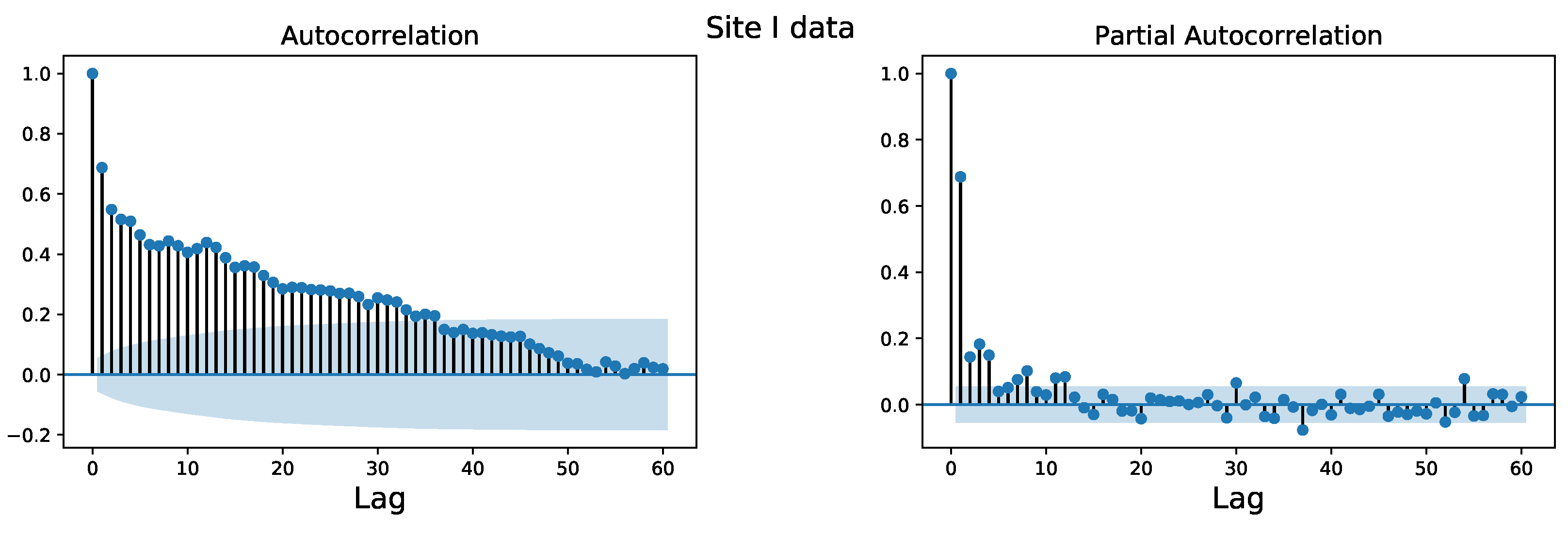
3.3. Data Description

For this study, we obtained real wind power data from three groups of wind farm sites located in the Adama district, Ethiopia. The data covers a four-year period, from 9 February 2019 to 25 July 2022, with the daily resolution for each wind farm (Site I, Site II, and Site III). To obtain the data, we sent an official letter to the Ethiopian electric power company and received approvals. The collected data were in their original format and the author took measures to maintain confidentiality and validity while processing the data. The wind farm is located in the Oromia Regional State and has a geographical location of 39 13 48 E latitude and 8 32 41 N longitude. It spans an area of 400–600 m wide and 5 km long, and is 95 km from the capital city of Ethiopia, Addis Ababa. To better understand the patterns in the data, we conducted an exploratory data analysis, including visualizing the time-based wind power generation trend. Figure 4 shows the daily wind energy generation capacity for each of the selected wind farms.
As depicted in Figure 4, the daily wind power output varies at each site, primarily due to the intermittency of wind speeds at each wind farm location. It can be noted that Site II and Site III often have even higher daily wind power generation, reaching up to 300,000 kW on certain days. In comparison, Site I has the highest wind generation capacity of 250,000 kW on some days, which is slightly lower than that of Sites II and III.
When forecasting time series problems, such as wind power, autocorrelation analysis is utilized to identify patterns and assess the randomness, stationarity, and other characteristics of the data. Moreover, the autocorrelation function (ACF) quantifies the linear relationship between the time series data and its lagged values, as outlined in Equation (14).
r k = t = k + 1 n ( y t y ¯ ) ( y t k y ¯ ) t = 1 n ( y t y ¯ ) 2
where r k represents the autocorrelation with a lag of k, and n represents the number of observations in the time series. Furthermore, y t refers to the actual data point at time t, and y ¯ denotes the sample average.
The autocorrelation value for wind power generation at Site I (as shown in Figure 5) exhibits high peaks at lag 1 and lag 2, then decreases gradually as the lag value increases up to 33 days. The autocorrelation plot confirms that the previous 30 lags of wind power values are highly correlated with each other and the trend is statistically significant in the subsequent series.
The autocorrelation plot for daily wind power production shown in Figure 6 reveals that most of the spikes are statistically significant, except for lag 29. This confirms that the time series data of wind power production are strongly correlated with its lag values, as depicted in Figure 6.
As illustrated in Figure 7, the wind power production data for Site III indicate that there are only strong correlations up to lag 19. Beyond that, as the lags increase, the statistical significance of the data decreases.

3.4. Data Pre-Processing

In our dataset, some of the wind power variables have missing values which need to be properly addressed to enhance the statistical power of the proposed model. To address this issue, the missing values were replaced using the K-nearest neighbor (KNN) imputation technique. KNN is a suitable imputation method that replaces missing observations for a given variable with the average of the values of its neighboring observations. The missing values were determined by calculating the distance between the missing observation on the variable and other observed values using the Euclidean distance formula, as expressed by Equation (15).
D ( x m , x o ) = i = 1 n x m i x o i
where x m i is the value of variable i in the target observation x m , x o i is the value of variable i in the other observed value x o , and D ( x m , x o ) is the distance between the target observation and the observed value.
The dataset was transferred from the Supervisory Control and Data Acquisition (SCADA) system to the report database through manual processing, which led to the discovery of numerous duplicate records in the dataset. These duplicate data values were then identified and removed using filtering techniques.
During the training of a deep learning model, some variables may have large numeric values which dominate the values of other variables, causing instability in the model training and leading to a large error gradient. To avoid this, it is important to perform feature scaling, which transforms the data into a normal or similar range, e.g., (0, 1), to ensure that the values of the dominating attributes do not overpower the values of smaller attributes. This also helps the gradient descent to converge more easily [47] and improves the model’s prediction performance. To achieve this, the min-max normalization method was employed in this paper to transform the data into the range (0, 1), as expressed by Equation (16).
X n = X 0 X m i n X m a x X m i n
where X n are the values of X after normalization, X 0 is a current value for variable X. X m i n and X m a x are the minimum and maximum data points in the variable X of the input dataset.

3.5. Problem Formulation

If we have real wind power data measured every day to forecast wind power for the next days, we use n different time steps with different data points at each time step. In our case, let X be the time series wind power data generated at time stamps X t = x 1 , x 2 , , x t . The one-step-ahead forecasting can incorporate the input features of the previous wind power and the prediction model can be expressed as shown in Equation (17).
x ^ t + 1 = f ( x t , x t 1 , , x t d + 1 )
where f is the model to be found and d is the number of lags considered for predicting x ^ t + 1 .

3.6. Performance Evaluation

The accuracy of the proposed model can be evaluated by comparing its predictions with real data using regression metrics. The statistical metrics used in this study are mean absolute error (MAE), root mean square error (RMSE), and mean absolute percentage error (MAPE), defined in Equations (18)–(20), respectively. MAE measures the difference between the predicted and actual values and is less sensitive to noisy data compared to RMSE. RMSE is the square root of the mean of the squared deviation between the predicted and actual values. However, RMSE is sensitive to the size of squared error outliers [35] and, therefore, may be negatively impacted by noisy data.
M A E = 1 n i = 1 n y y ^
R M S E = 1 n i = 1 n y y ^ 2
M A P E = 1 n i = 1 n | y y ^ | y 100
where y and y ^ represent the actual and predicted values, respectively. In addition, n represents the total number of observations used to train the model.

4. Results Discussion

In this paper, a set of hyperparameters used to tune the proposed models is defined with a range of values or categorical values. The LSTM model is built using these hyperparameters, and the optimal values are searched from the hyperparameter space using the Bayesian optimization algorithm. The hyperparameters for epochs and batch size were selected as 80 and 32, respectively, with a greater emphasis on improving the model. The model was constructed with two LSTM hidden layers, and the optimal number of neurons in the first and second hidden layers were 120 and 20, respectively. The optimal activation function selected in each hidden layer is the tangent function, named t a n h , while the activation function in the output layer is a linear function that sums up the weighted total of the inputs and returns the result. The best optimizer, RMSprop, was selected from the given hyperparameter spaces with a learning rate of 0.01 (Table 1).
The selection of hyperparameters for BO-LSTM and BO-GRU is done by defining the same hyperparameter space with the range values as presented in Table 1. The optimal parameters for each deep learning algorithm are different, except for the same epoch and batch size values of 80 and 32, respectively, which were optimally selected for both algorithms. For example, the best activation function selected by Bayesian optimization for BO-GRU is ReLu, whereas the t a n h function was selected as the optimal activation function for BO-LSTM. The parameters for the rest of the benchmark models were chosen manually, as shown in Table 2.
Overfitting is a common problem in machine learning where a model performs well on the training data, but poorly on new, unseen data. This can occur when the model is too complex and has too many parameters relative to the size of the training data. The model ends up learning the noise in the training data rather than the underlying relationship. To prevent such an undesirable effect, two main actions have been taken. First, L1 regularization technique has been used to reduce the complexity of the model. Second, the model has been run for only 80 epochs, stopping the training process before the model becomes too complex.
Figure 8 displays the training and validation loss for the BO-LSTM model. Figure 8a,b demonstrate the model’s ability to learn the wind power data from Site I and Site II, respectively. As the number of epochs increases, it can be seen that the training and validation loss decrease and converge well. However, the convergence is better for Site I data in Figure 8a compared to Site II data in Figure 8b. This indicates that the model learns from Site I data more effectively than from Site II data. In contrast, the training curve in Figure 8b appears correct, but the validation curve becomes noisy, especially up to 45 iterations, potentially due to the validation data not being representative of the training data.
As depicted in Figure 9a,b, the training curve and the validation curve diverge. Specifically, in Figure 9b, the divergence is significant starting from the first epoch, whereas in Figure 9a, the training and validation curves bear some resemblance.
Table 3 summarizes the forecast results achieved by the proposed method in terms of the evaluation metrics introduced in Section 3.6. In order to assess its effectiveness, results for other well-established methods were selected: standard neural networks (ANN), other deep learning models (GRU), ensemble learning (XGBoost) or standard statistical methods (ARIMA). From Table 3, it can be observed that all the nonlinear models (ANN, LSTM, GRU, BO-LSTM, and BO-GRU) outperform the linear ones i.e ARIMA and XGBoost in terms of all three metrics in all cases data. This is due to the fact that wind power time series data show non-linearity and non-stationarity properties (see Figure 5, Figure 6 and Figure 7) and these conventional machine learning models are incapable of handling the nonlinear relation of the time series data. On the other hand, the fitting ability of deep learning methods is superior for complex time series forecasting tasks [33].
Moreover, hyperparameter tuning has a significant effect on the performance of these nonlinear models and BO-LSTM and BO-GRU outperform the standard LSTM and GRU. It can be observed that the performance of BO-LSTM is better than all benchmark algorithms such ANN, XGBoost, ARIMA, standard LSTM, and BO-GRU according to all error indices and for the three wind farm sites dataset, except the slightly lower MAE error value of the competitive BO-GRU for Site II. Specifically, while comparing with standard LSTM and BO-GRU in all three cases, BO-LSTM obtained lower MAE, RMSE, and MAPE error with values of 0.0621, 0.0793, and 1.1353, respectively, for Site I. However, the differences in prediction accuracy between BO-LSTM and BO-GRU are not very large. Hence, Table 3 shows the viability of a Bayesian Optimization algorithm in tuning the LSTM model by searching for the best hyperparameter combination which significantly improves the proposed BO-LSTM performance.
Table 4 shows the error indices of the optimized deep learning frameworks, namely BO-LSTM and BO-GRU models, and the standard LSTM and GRU on both the training and test data. The MAE and RMSE error values for all three cases are very much closer and lower than that of the use of untuned deep learning models. It can be observed that by applying the hyperparameter tuning prior to building deep learning models, they learn nonlinear features from wind power and reduces the overfitting problems that have been experienced with the use of standard LSTM and GRU implementation. Moreover, from the analysis of Table 4, it is worth mentioning that BO-LSTM achieves superior performance than that of the standard LSTM and BO-GRU models, both on training and test MAE and RMSE metrics for all three cases.
As shown, the BO-LSTM model outperforms the BO-GRU model. Both BO-LSTM and BO-GRU models were applied to the data from the three wind farm sites or groups, as indicated in Table 3. It can be concluded that Bayesian optimization is a suitable strategy for this context, as both deep learning models show competitive results when optimized in this way. Despite using the same optimization strategy to search for optimal parameters in the same hyperparameter spaces, as shown in Table 1 and Table 2, the prediction errors still varied, which could be due to the variability of the data recorded at each wind generation plant. The BO-LSTM-based prediction results are presented in Figure 10, Figure 11 and Figure 12 for the actual and predicted data of Site I, Site II, and Site III, respectively. These figures show a good resemblance between the actual and predicted data, as confirmed in Table 4. The Supplementary Material, including the actual and predicted values for these figures, can be found at https://github.com/DataLabUPO/AdamaWindPowerResults, accessed on 19 February 2023.

5. Conclusions

In this paper, we use the Bayesian optimization algorithm to find the optimal hyperparameter values that result in a higher level of model accuracy. We search for impactful hyperparameter values and use them to develop deep LSTM and deep GRU models on a real wind power dataset. For each selected wind farm site, we propose and test wind power forecasting models. Our experimental results and comparative analysis show that the proposed model, which combines Bayesian Optimization and deep LSTM, outperforms the benchmark models in terms of error metrics. Hyperparameter tuning with Bayesian Optimization is a feasible method that finds the optimal combination of parameters within a reasonable computation time. It also helps to minimize model overfitting issues. The results in Table 4 show that the training and test error variance for the BO-LSTM model is much lower than for the standard LSTM network. Additionally, conventional machine learning models and ANNs cannot discover the temporal information hidden in wind power time series data, leading to inaccurate estimations. However, despite the difficulty and time consumption of training deep learning models, the combination of Bayesian Optimization and deep LSTM is found to be efficient and effective in learning nonlinear time series data. In comparison to the baseline ANN, XGBoost, and ARIMA models, the BO-LSTM model achieves better results. Additionally, it outperforms tuned GRU models in terms of performance on training and test data with good learning convergence. In wind power forecasting, time is an important feature to predict future sequence values and future work should address this parameter through automatic hyperparameter tuning, which is not covered in this work. The proposed BO-LSTM model can also be tested with a particular location’s exogenous variables, such as temperature, wind speed, and wind direction in addition to the wind power variable in future work.

Supplementary Materials

The following supporting information can be downloaded at: https://github.com/DataLabUPO/AdamaWindPowerResults, accessed on 19 February 2023.

Author Contributions

E.T.H. designed the methodology, wrote the article, and conducted the experimentation. F.M.-Á. supervised and was involved in writing and editing the article. K.K. supervised the topic selection and conceptual development. M.M.-B. wrote the literature, designed the models, and edited the methodology. All authors have read and agreed to the published version of the manuscript.

Funding

The authors would like to express their gratitude to the Spanish Ministry of Science and Innovation for their support through projects PID2020-117954RB and TED2021-131311B-C22. They would also like to thank the European Regional Development Fund and Junta de Andalucía for their support through projects PY20-00870 and UPO-138516.

Data Availability Statement

Data are available upon request to the Ethiopian Electric Utility company.

Conflicts of Interest

The authors declare no conflict of interest regarding the publication of this paper.

Acronym

ANNartificial neural network
ARIMAautoregressive integrative moving average
BO-LSTMBayesian optimized long short-term memory
GRUgated recurrent unit
KNNK-nearest neighbor
LSTMLong-short term memory
MAEmean absolute error
MAPEmean absolute percentage error
RNNrecurrent neural network
RMSEroot mean square error
SCADAsupervisory control and data acquisition
SVMsupport vector machine

References

  1. Yürek, Ö.; Birant, D.; Yürek, İ. Wind Power Generation Prediction Using Machine Learning Algorithms. Dokuz Eylül Üniversitesi Mühendislik Fakültesi Fen Mühendislik Derg. 2021, 23, 107–119. [Google Scholar]
  2. Khan, N.; Ullah, F.U.M.; Haq, I.U.; Khan, S.U.; Lee, M.Y.; Baik, S.W. AB-net: A novel deep learning assisted framework for renewable energy generation forecasting. Mathematics 2021, 9, 2456. [Google Scholar] [CrossRef]
  3. Shahiduzzaman, K.M.; Jamal, M.N.; Nawab, M.R.I. Renewable Energy Production Forecasting: A Comparative Machine Learning Analysis. Int. J. Eng. Adv. Technol. 2021, 10, 11–18. [Google Scholar] [CrossRef]
  4. Mishra, S.; Bordin, C.; Taharaguchi, K.; Palu, I. Comparison of deep learning models for multivariate prediction of time series wind power generation and temperature. Energy Rep. 2020, 6, 273–286. [Google Scholar] [CrossRef]
  5. Delgado, I.; Fahim, M. Wind turbine data analysis and LSTM-based prediction in SCADA system. Energies 2020, 14, 125. [Google Scholar] [CrossRef]
  6. Tiruye, G.A.; Besha, A.T.; Mekonnen, Y.S.; Benti, N.E.; Gebreslase, G.A.; Tufa, R.A. Opportunities and Challenges of Renewable Energy Production in Ethiopia. Sustainability 2021, 13, 10381. [Google Scholar] [CrossRef]
  7. Zhang, P.; Wang, Y.; Liang, L.; Li, X.; Duan, Q. Short-term wind power prediction using GA-BP neural network based on DBSCAN algorithm outlier identification. Processes 2020, 8, 157. [Google Scholar] [CrossRef] [Green Version]
  8. Prema, V.; Bhaskar, M.S.; Almakhles, D.; Gowtham, N.; Rao, K.U. Critical Review of Data, Models and Performance Metrics for Wind and Solar Power Forecast. IEEE Access 2021, 10, 667–688. [Google Scholar] [CrossRef]
  9. Shahid, F.; Zameer, A.; Muneeb, M. A novel genetic LSTM model for wind power forecast. Energy 2021, 223, 120069. [Google Scholar] [CrossRef]
  10. Alkhayat, G.; Mehmood, R. A review and taxonomy of wind and solar energy forecasting methods based on deep learning. Energy AI 2021, 4, 100060. [Google Scholar] [CrossRef]
  11. Torres, J.F.; Hadjout, D.; Sebaa, A.; Martínez-Álvarez, F.; Troncoso, A. Deep learning for time series forecasting: A survey. Big Data 2021, 9, 3–21. [Google Scholar] [CrossRef]
  12. Victoria, A.H.; Maragatham, G. Automatic tuning of hyperparameters using Bayesian optimization. Evol. Syst. 2021, 12, 217–223. [Google Scholar] [CrossRef]
  13. Paramasivan, S.K. Deep Learning Based Recurrent Neural Networks to Enhance the Performance of Wind Energy Forecasting: A Review. Rev. d’Intelligence Artif. 2021, 35, 1–10. [Google Scholar] [CrossRef]
  14. Hossain, M.A.; Chakrabortty, R.K.; Elsawah, S.; Gray, E.M.; Ryan, M.J. Predicting wind power generation using hybrid deep learning with optimization. IEEE Trans. Appl. Supercond. 2021, 31, 0601305. [Google Scholar] [CrossRef]
  15. Shamshirband, S.; Rabczuk, T.; Chau, K.W. A survey of deep learning techniques: Application in wind and solar energy resources. IEEE Access 2019, 7, 164650–164666. [Google Scholar] [CrossRef]
  16. Peng, L.; Wang, L.; Xia, D.; Gao, Q. Effective energy consumption forecasting using empirical Wavelet transform and Long Short-Term Memory. Energy 2022, 238, 121756. [Google Scholar] [CrossRef]
  17. Khalid, R.; Javaid, N. A survey on hyperparameters optimization algorithms of forecasting models in smart grid. Sustain. Cities Soc. 2020, 61, 102275. [Google Scholar] [CrossRef]
  18. Perrone, V.; Shen, H.; Seeger, M.W.; Archambeau, C.; Jenatton, R. Learning search spaces for bayesian optimization: Another view of hyperparameter transfer learning. Adv. Neural Inf. Process. Syst. 2019, 32, 1–11. [Google Scholar]
  19. Yue, W.; Liu, Q.; Ruan, Y.; Qian, F.; Meng, H. A prediction approach with mode decomposition-recombination technique for short-term load forecasting. Sustain. Cities Soc. 2022, 85, 104034. [Google Scholar] [CrossRef]
  20. Wu, J.; Chen, X.Y.; Zhang, H.; Xiong, L.D.; Lei, H.; Deng, S.H. Hyperparameter optimization for machine learning models based on Bayesian optimization. J. Electron. Sci. Technol. 2019, 17, 26–40. [Google Scholar]
  21. Shekhar, S.; Bansode, A.; Salim, A. A Comparative study of Hyper-Parameter Optimization Tools. In Proceedings of the 2021 IEEE Asia-Pacific Conference on Computer Science and Data Engineering (CSDE), Brisbane, Australia, 8–10 December 2021; pp. 1–6. [Google Scholar]
  22. Blanchard, A.; Sapsis, T. Bayesian optimization with output-weighted optimal sampling. J. Comput. Phys. 2021, 425, 109901. [Google Scholar] [CrossRef]
  23. Yang, Y.; Haq, E.U.; Jia, Y. A Novel Deep Learning Approach for Short and Medium-Term Electrical Load Forecasting Based on Pooling LSTM-CNN Model. In Proceedings of the 2020 IEEE/IAS Industrial and Commercial Power System Asia (I&CPS Asia), Weihai, China, 13–15 July 2020; pp. 26–34. [Google Scholar]
  24. Li, C.; Tang, G.; Xue, X.; Saeed, A.; Hu, X. Short-term wind speed interval prediction based on ensemble GRU model. IEEE Trans. Sustain. Energy 2019, 11, 1370–1380. [Google Scholar] [CrossRef]
  25. Kedia, A.; Sanyal, A.; Gogoi, A.; Kumar, A.; Goswani, A.K.; Tiwari, P.K.; Choudhury, N.B.D. Wind Power Uncertainties Forecasting based on Long Short Term Memory Model for Short-Term Power Market. In Proceedings of the 2020 IEEE First International Conference on Smart Technologies for Power, Energy and Control (STPEC), Bilaspur, India, 19–22 December 2020; pp. 1–6. [Google Scholar] [CrossRef]
  26. Dolatabadi, A.; Abdeltawab, H.; Mohamed, Y.A.R.I. Hybrid deep learning-based model for wind speed forecasting based on DWPT and bidirectional LSTM network. IEEE Access 2020, 8, 229219–229232. [Google Scholar] [CrossRef]
  27. Hossain, M.A.; Chakrabortty, R.K.; Elsawah, S.; Ryan, M.J. Very short-term forecasting of wind power generation using hybrid deep learning model. J. Clean. Prod. 2021, 296, 126564. [Google Scholar] [CrossRef]
  28. Chen, H.; Birkelund, Y.; Zhang, Q. Data-augmented sequential deep learning for wind power forecasting. Energy Convers. Manag. 2021, 248, 114790. [Google Scholar] [CrossRef]
  29. Duan, J.; Wang, P.; Ma, W.; Fang, S.; Hou, Z. A novel hybrid model based on nonlinear weighted combination for short-term wind power forecasting. Int. J. Electr. Power Energy Syst. 2022, 134, 107452. [Google Scholar] [CrossRef]
  30. Wang, Z.; Zhang, J.; Zhang, Y.; Huang, C.; Wang, L. Short-term wind speed forecasting based on information of neighboring wind farms. IEEE Access 2020, 8, 16760–16770. [Google Scholar] [CrossRef]
  31. Khodayar, M.; Wang, J. Spatio-Temporal Graph Deep Neural Network for Short-Term Wind Speed Forecasting. IEEE Trans. Sustain. Energy 2019, 10, 670–681. [Google Scholar] [CrossRef]
  32. Optis, M.; Perr-Sauer, J. The importance of atmospheric turbulence and stability in machine-learning models of wind farm power production. Renew. Sustain. Energy Rev. 2019, 112, 27–41. [Google Scholar] [CrossRef]
  33. Wang, Y.; Zou, R.; Liu, F.; Zhang, L.; Liu, Q. A review of wind speed and wind power forecasting with deep neural networks. Appl. Energy 2021, 304, 117766. [Google Scholar] [CrossRef]
  34. Ju, J.; Liu, K.; Liu, F. Prediction of SO2 Concentration Based on AR-LSTM Neural Network. Neural Process. Lett. 2022. [Google Scholar] [CrossRef]
  35. Ahmed, S.I.; Ranganathan, P.; Salehfar, H. Forecasting of Mid-and Long-Term Wind Power Using Machine Learning and Regression Models. In Proceedings of the 2021 IEEE Kansas Power and Energy Conference (KPEC), Manhattan, KS, USA, 19–20 April 2021; pp. 1–6. [Google Scholar]
  36. Eyecioglu, O.; Hangun, B.; Kayisli, K.; Yesilbudak, M. Performance comparison of different machine learning algorithms on the prediction of wind turbine power generation. In Proceedings of the 2019 8th IEEE International Conference on Renewable Energy Research and Applications (ICRERA), Brasov, Romania, 3–6 November 2019; pp. 922–926. [Google Scholar]
  37. Shabbir, N.; AhmadiAhangar, R.; Kütt, L.; Iqbal, M.N.; Rosin, A. Forecasting short term wind energy generation using machine learning. In Proceedings of the 2019 IEEE 60th International Scientific Conference on Power and Electrical Engineering of Riga Technical University (RTUCON), Riga, Latvia, 7–9 October 2019; pp. 1–4. [Google Scholar]
  38. Wei, D.; Wang, J.; Niu, X.; Li, Z. Wind speed forecasting system based on gated recurrent units and convolutional spiking neural networks. Appl. Energy 2021, 292, 116842. [Google Scholar] [CrossRef]
  39. Qiao, L.; Chen, S.; Bo, J.; Liu, S.; Ma, G.; Wang, H.; Yang, J. Wind power generation forecasting and data quality improvement based on big data with multiple temporal-spatial scale. In Proceedings of the IEEE International Conference on Energy Internet, Nanjing, China, 27–31 May 2019; pp. 554–559. [Google Scholar]
  40. Gao, X. Monthly Wind Power Forecasting: Integrated Model Based on Grey Model and Machine Learning. Sustainability 2022, 14, 15403. [Google Scholar] [CrossRef]
  41. Ye, J.; Xie, L.; Ma, L.; Bian, Y.; Xu, X. A novel hybrid model based on Laguerre polynomial and multi-objective Runge–Kutta algorithm for wind power forecasting. Int. J. Electr. Power Energy Syst. 2023, 146, 108726. [Google Scholar] [CrossRef]
  42. Peng, X.; Wang, H.; Lang, J.; Li, W.; Xu, Q.; Zhang, Z.; Cai, T.; Duan, S.; Liu, F.; Li, C. EALSTM-QR: Interval wind-power prediction model based on numerical weather prediction and deep learning. Energy 2021, 220, 119692. [Google Scholar] [CrossRef]
  43. Wang, R.; Li, C.; Fu, W.; Tang, G. Deep learning method based on gated recurrent unit and variational mode decomposition for short-term wind power interval prediction. IEEE Trans. Neural Netw. Learn. Syst. 2019, 31, 3814–3827. [Google Scholar] [CrossRef]
  44. Afrasiabi, M.; Mohammadi, M.; Rastegar, M.; Afrasiabi, S. Advanced deep learning approach for probabilistic wind speed forecasting. IEEE Trans. Ind. Inform. 2020, 17, 720–727. [Google Scholar] [CrossRef]
  45. Yu, R.; Gao, J.; Yu, M.; Lu, W.; Xu, T.; Zhao, M.; Zhang, J.; Zhang, R.; Zhang, Z. LSTM-EFG for wind power forecasting based on sequential correlation features. Future Gener. Comput. Syst. 2019, 93, 33–42. [Google Scholar] [CrossRef]
  46. Basu, S.; Watson, S.J.; Arends, E.L.; Cheneka, B. Day-ahead Wind Power Predictions at Regional Scales: Post-processing Operational Weather Forecasts with a Hybrid Neural Network. In Proceedings of the 2020 17th IEEE International Conference on the European Energy Market (EEM), Stockholm, Sweden, 16–18 September 2020; pp. 1–6. [Google Scholar]
  47. Meng, X.; Wang, R.; Zhang, X.; Wang, M.; Ma, H.; Wang, Z. Hybrid Neural Network Based on GRU with Uncertain Factors for Forecasting Ultra-short-term Wind Power. In Proceedings of the 2020 IEEE 2nd International Conference on Industrial Artificial Intelligence (IAI), Shenyang, China, 23–25 October 2020; pp. 1–6. [Google Scholar]
  48. Wang, H.K.; Song, K.; Cheng, Y. A Hybrid Forecasting Model Based on CNN and Informer for Short-Term Wind Power. Front. Energy Res. 2022, 9, 1041. [Google Scholar] [CrossRef]
  49. Lv, J.; Zheng, X.; Pawlak, M.; Mo, W.; Miśkowicz, M. Very short-term probabilistic wind power prediction using sparse machine learning and nonparametric density estimation algorithms. Renew. Energy 2021, 177, 181–192. [Google Scholar] [CrossRef]
  50. Akbal, Y.; Ünlü, K.D. A univariate time series methodology based on sequence-to-sequence learning for short to midterm wind power production. Renew. Energy 2022, 200, 832–844. [Google Scholar] [CrossRef]
  51. Liu, Z.; Li, Y.; Yao, J.; Cai, Z.; Han, G.; Xie, X. Ultra-short-term Forecasting Method of Wind Power Based on W-BiLSTM. In Proceedings of the 2021 IEEE 4th International Electrical and Energy Conference (CIEEC), Wuhan, China, 28–30 May 2021; pp. 1–6. [Google Scholar] [CrossRef]
  52. Xia, M.; Shao, H.; Ma, X.; de Silva, C.W. A Stacked GRU-RNN-Based Approach for Predicting Renewable Energy and Electricity Load for Smart Grid Operation. IEEE Trans. Ind. Inform. 2021, 17, 7050–7059. [Google Scholar] [CrossRef]
  53. Putz, D.; Gumhalter, M.; Auer, H. A novel approach to multi-horizon wind power forecasting based on deep neural architecture. Renew. Energy 2021, 178, 494–505. [Google Scholar] [CrossRef]
  54. Lin, W.H.; Wang, P.; Chao, K.M.; Lin, H.C.; Yang, Z.Y.; Lai, Y.H. Wind power forecasting with deep learning networks: Time-series forecasting. Appl. Sci. 2021, 11, 10335. [Google Scholar] [CrossRef]
  55. Prema, V.; Sarkar, S.; Rao, K.U.; Umesh, A. LSTM based Deep Learning model for accurate wind speed prediction. Data Sci. Mach. Learn 2019, 1, 6–11. [Google Scholar]
  56. Yi, L.; Sun, H.; Qiu, D.; Chen, Z.; Chang, F.; Zhao, J. Short-term Wind Power Forecasting with Evolutionary Deep Learning. In Proceedings of the 2019 IEEE 3rd Conference on Energy Internet and Energy System Integration (EI2), Beijing, China, 20–22 October 2019; pp. 1508–1513. [Google Scholar]
  57. Dehnavi, S.D.; Shirani, A.; Mehrjerdi, H.; Baziar, M.; Chen, L. New Deep Learning-Based Approach for Wind Turbine Output Power Modeling and Forecasting. IEEE Trans. Ind. Appl. 2020. [Google Scholar] [CrossRef]
  58. Akash, R.; Rangaraj, A.; Meenal, R.; Lydia, M. Machine learning based univariate models for long term wind speed forecasting. In Proceedings of the 2020 IEEE International Conference on Inventive Computation Technologies (ICICT), Coimbatore, India, 26–28 February 2020; pp. 779–784. [Google Scholar]
  59. Rahaman, H.; Bashar, T.R.; Munem, M.; Hasib, M.H.H.; Mahmud, H.; Alif, A.N. Bayesian Optimization Based ANN Model for Short Term Wind Speed Forecasting in Newfoundland, Canada. In Proceedings of the 2020 IEEE Electric Power and Energy Conference (EPEC), Virtual, 22–31 October 2020; pp. 1–5. [Google Scholar]
  60. Saini, V.K.; Bhardwaj, B.; Gupta, V.; Kumar, R.; Mathur, A. Gated Recurrent Unit (GRU) Based Short Term Forecasting for Wind Energy Estimation. In Proceedings of the 2020 IEEE International Conference on Power, Energy, Control and Transmission Systems (ICPECTS), Chennai, India, 10–11 December 2020; pp. 1–6. [Google Scholar]
  61. Wu, L.; Kong, C.; Hao, X.; Chen, W. A short-term load forecasting method based on GRU-CNN hybrid neural network model. Math. Probl. Eng. 2020, 2020, 1428104. [Google Scholar] [CrossRef] [Green Version]
  62. Yang, J.; Tan, K.K.; Santamouris, M.; Lee, S.E. Building energy consumption raw data forecasting using data cleaning and deep recurrent neural networks. Buildings 2019, 9, 204. [Google Scholar] [CrossRef] [Green Version]
  63. Hadjout, D.; Torres, J.F.; Troncoso, A.; Sebaa, A.; Martínez-Álvarez, F. Electricity consumption forecasting based on ensemble deep learning with application to the Algerian market. Energy 2022, 243, 123060. [Google Scholar] [CrossRef]
  64. Saini, V.K.; Kumar, R.; Mathur, A.; Saxena, A. Short term forecasting based on hourly wind speed data using deep learning algorithms. In Proceedings of the 2020 3rd IEEE International Conference on Emerging Technologies in Computer Engineering: Machine Learning and Internet of Things (ICETCE), Jaipur, India, 7–8 February 2020; pp. 1–6. [Google Scholar]
  65. Rafi, S.H.; Deeba, S.R.; Hossain, E. A short-term load forecasting method using integrated CNN and LSTM network. IEEE Access 2021, 9, 32436–32448. [Google Scholar] [CrossRef]
  66. Rafi, S.H. Highly Efficient Short Term Load Forecasting Scheme Using Long Short Term Memory Network. In Proceedings of the 2020 8th IEEE International Electrical Engineering Congress (iEECON), Chiang Mai, Thailand, 4–6 March 2020; pp. 1–4. [Google Scholar]
  67. Bui, K.T.T.; Torres, J.F.; Gutiérrez-Avilés, D.; Nhu, V.H.; Martínez-Álvarez, F.; Bui, D.T. Deformation forecasting of a hydropower dam by hybridizing a Long Short-Term Memory deep learning network with the Coronavirus Optimization Algorithm. Comput.-Aided Civ. Infrastruct. Eng. 2021, 37, 1368–1386. [Google Scholar] [CrossRef]
  68. Torres, J.F.; Martínez-Álvarez, F.; Troncoso, A. A deep LSTM network for the Spanish electricity consumption forecasting. Neural Comput. Appl. 2022, 34, 10533–10545. [Google Scholar] [CrossRef]
  69. Rahman, M.O.; Hossain, M.S.; Junaid, T.S.; Forhad, M.S.A.; Hossen, M.K. Predicting prices of stock market using gated recurrent units (GRUs) neural networks. Int. J. Comput. Sci. Netw. Secur 2019, 19, 213–222. [Google Scholar]
  70. Zhou, X.; Xu, J.; Zeng, P.; Meng, X. Air pollutant concentration prediction based on GRU method. J. Phys. Conf. Ser. 2019, 1168, 032058. [Google Scholar]
  71. Liu, H.; Shen, L. Forecasting carbon price using empirical wavelet transform and gated recurrent unit neural network. Carbon Manag. 2020, 11, 25–37. [Google Scholar] [CrossRef]
  72. Yang, T.; Li, B.; Xun, Q. LSTM-attention-embedding model-based day-ahead prediction of photovoltaic power output using Bayesian optimization. IEEE Access 2019, 7, 171471–171484. [Google Scholar] [CrossRef]
  73. Jiménez-Navarro, M.J.; Martínez-Álvarez, F.; Troncoso, A.; Asencio-Cortés, G. HLNet: A Novel Hierarchical Deep Neural Network for Time Series Forecasting. Adv. Intell. Syst. Comput. 2021, 1401, 717–727. [Google Scholar]
  74. Abdalla, E.M.H.; Pons, V.; Stovin, V.; De-Ville, S.; Fassman-Beck, E.; Alfredsen, K.; Muthanna, T.M. Evaluating different machine learning methods to simulate runoff from extensive green roofs. Hydrol. Earth Syst. Sci. 2021, 25, 5917–5935. [Google Scholar] [CrossRef]
  75. Sultana, N.; Hossain, S.; Almuhaini, S.H.; Düştegör, D. Bayesian Optimization Algorithm-Based Statistical and Machine Learning Approaches for Forecasting Short-Term Electricity Demand. Energies 2022, 15, 3425. [Google Scholar] [CrossRef]
Figure 1. Proposed methodology for wind power forecasting.
Energies 16 02317 g001
Figure 2. LSTM architecture.
Energies 16 02317 g002
Figure 3. GRU architecture.
Energies 16 02317 g003
Figure 4. Daily wind generation capacity by three wind farms Sites.
Energies 16 02317 g004
Figure 5. Autocorrelation (left) and Partial Autocorrelation (right) for Site I.
Energies 16 02317 g005
Figure 6. Autocorrelation (left) and partial autocorrelation (right) for Site II.
Energies 16 02317 g006
Figure 7. Autocorrelation (left) and partial autocorrelation (right) for Site III.
Energies 16 02317 g007
Figure 8. Training vs. validation loss based on BO-LSTM. (a) Training vs. validation loss for Site I. (b) Training vs. validation loss for Site II.
Energies 16 02317 g008
Figure 9. Training vs. validation loss without LSTM Model tuning. (a) Training vs. validation loss for Site I. (b) Training vs. validation loss for Site II.
Energies 16 02317 g009
Figure 10. Prediction vs. actual plot for Site I.
Energies 16 02317 g010
Figure 11. Prediction vs. actual plot for Site II.
Energies 16 02317 g011
Figure 12. Prediction vs. actual plot for Site III.
Energies 16 02317 g012
Table 1. Set of hyperparameters spaces for LSTM and GRU Models.
HyperparametersRange ValuesOptimal Parameters Selected by Bayesian Optimization
Learning rate 0.0001 , 0.001 , 0.01 , 0.1 , 0.2 0.01
Epochs 40 , 60 , 80 , 100 , 120 80
Batch size 8 , 16 , 32 , 64 32
Dropout 0.1 , 0.2 , 0.4 , 0.6 0.2
Activation function R e L u , t a n h , l i n e a r tanh
Optimizer A d a m , R M S p r o p , A d a d e l t a RMSprop
Neurons 40 , 60 , 80 , 100 , 120 , 20 , 40 , 60 , 80 , 100 120 , 20
Table 2. Hyperparameters for the baseline models.
ModelsParametersValues/Type
ANNEpoch4
Learning rate0.001
Batch size32
Neuron at hidden layer20
OptimizerAdam
Activation functionReLu
XGBoostn_estimators116
Learning rate0.3
max_depth3
gamma5
min_child_weight6
colsample_bytree0.6
ARIMAP4
d0
q1
GRULearning _rate0.0001
Batch size32
Epoch80
Neuron at hidden layers100, 20
Dropout_rate0.1
Activation functionReLu
OptimizerAdam
LSTMLearning_rate0.001
Batch size32
Neuron at hidden layer20
Activation functionReLu
OptimizerAdam
Table 3. Comparison of six forecasting models on three Sites data.
DataModelsMAERMSEMAPE (%)
Site IANN0.10090.13100.916
XGBoost0.13120.16641.3737
ARIMA0.19390.22771.8680
LSTM0.10700.12642.0642
BO-GRU0.06510.08261.1470
BO-LSTM0.06210.07931.1353
Site IIANN0.10240.13072.4062
XGBoost0.14890.19261.7796
ARIMA0.18440.22142.2057
LSTM0.11370.13991.1725
BO-GRU0.07070.09101.1621
BO-LSTM0.07080.08931.2275
Site IIIANN0.14400.17911.9741
XGBoost0.14520.18781.6768
ARIMA0.17480.21062.1963
LSTM0.11370.14011.1903
BO-GRU0.09720.12471.0896
BO-LSTM0.09480.12201.0674
Table 4. Forecasting performances of competitive deep learning models on training and test data.
DatasetModelsTrainingTesting
MAERMSEMAERMSE
Site ILSTM0.09090.11670.11180.1371
GRU0.08250.10460.10040.1205
BO-GRU0.06110.08070.06930.0881
BO-LSTM0.05900.07820.06270.0800
Site IILSTM0.08480.11040.09500.1146
GRU0.08750.11420.09700.1163
BO-GRU0.07140.09670.07750.0989
BO-LSTM0.06890.09560.07410.0930
Site IIILSTM0.11670.14610.10950.1386
GRU0.12190.15050.10880.1363
BO-GRU0.10630.13770.09930.1274
BO-LSTM0.10320.13520.09860.1258
Disclaimer/Publisher’s Note: The statements, opinions and data contained in all publications are solely those of the individual author(s) and contributor(s) and not of MDPI and/or the editor(s). MDPI and/or the editor(s) disclaim responsibility for any injury to people or property resulting from any ideas, methods, instructions or products referred to in the content.

