Abstract
Short-term hydrothermal scheduling problem plays an important role in maintaining a high degree of economy and reliability in power system operational planning. Since electric power generation from fossil fired plants forms a major part of hydrothermal generation mix, therefore their emission contributions cannot be neglected. Hence, multi-objective short term hydrothermal scheduling is formulated as a bi-objective optimization problem by considering (a) minimizing economical power generation cost, (b) minimizing environmental emission pollution, and (c) simultaneously minimizing both the conflicting objective functions. This paper presents a non-dominated sorting disruption-based oppositional gravitational search algorithm (NSDOGSA) to solve multi-objective short-term hydrothermal scheduling (MSHTS) problems and reveals that (i) the short-term hydrothermal scheduling problem is extended to a multi-objective short-term hydrothermal scheduling problem by considering economical production cost (EPC) and environmental pollution (EEP) simultaneously while satisfying various diverse constraints; (ii) by introducing the concept of non-dominated sorting (NS) in gravitational search algorithm (GSA), it can optimize two considered objectives such as EPC and EEP simultaneously and can also obtain a group of conflicting solutions in one trial simulation; (iii) in NSDOGSA, the objective function in terms fitness for mass calculation has been represented by its rank instead of its EPC & EEP values by using the NS approach; (iv) an elite external archive set is defined to keep the NS solutions with the idea of spread indicator; (v) the optimal schedule value is extracted by using fuzzy decision approach; (vi) a consistent handling strategy has been adopted to handle effectively the system constraints; (vii) finally, the NSDOGSA approach is verified on two test systems with valve point loading effects and transmission loss, and (viii) computational discussion show that the NSDOGSA gives improved optimal results in comparison to other existing methods, which qualifies that the NSDOGSA is an effective and competitive optimization approach for solving complex MSHTS problems.
1. Introduction
In modern power systems, the efficient dispatch of available power resources for satisfying the increased load has become an important aspect of economic operation of the power system. In this respect, hydro energy sources are considered to be promising alternative energy sources integrated with thermal plants to provide a clean, smooth, environment-friendly energy operation and also meet other requirements such as flood control and irrigation. Usually, the operation of a hydrothermal integrated system is more complex than the scheduling of an all-thermal generation system as the hydroelectric plants are coupled both electrically and hydraulically. Therefore, the optimum scheduling of hydrothermal generation plants is of utmost importance in the current scenario due to its economical aspect linked with the power system operation.
In the process of power system operation and planning, hydrothermal scheduling (HTS) is of a vital role to maintain a high degree of economy and reliability. The storage capacity of the reservoir is the deciding factor in whether long-term or short-term scheduling is desired for the operation planning of a hydrothermal power system. In long-term scheduling, the discharge rates at hydro stations and generation of thermal stations are determined on monthly intervals for an optimization period of several years so that the economical production cost of thermal generation is minimum. Such type of problem is a stochastic one because the load demand and inflows at various reservoirs over the period are not known exactly. On the other hand, the short-term scheduling problem is concerned with an available water allocation over a shorter period such as an hourly period that minimizes the overall thermal generation cost. The inclusion of time delays for water travel time between cascaded reservoirs is usually not necessary for the long-term problem; however, it is mandatory to consider them for short-term hydrothermal scheduling (SHTS) problems. SHTS issues are divided into fixed-head and variable-head problems. The SHTS issue may be divided into two categories based on the head of the reservoir: fixed head and variable head. Fixed head reservoirs have a big capacity, but variable head reservoirs have a restricted quantity of water. Reservoir head is almost constant for high-capacity reservoirs in SHTS problems due to low fluctuation of inflows. Even so, because of the considerable effect of inflows, head variation cannot be overlooked in small scale reservoirs. The hydro generation is assumed to be a function of water discharge quantities in fixed head SHTS formulation. The variable head scheduling issue, on the other hand, is concerned with the nonlinear function of hydropower in terms of reservoir storage and water discharge. Moreover, reservoir volume restrictions like as maximum and minimum limits are generally taken into account in variable head formulation. Variable head plant models also incorporate flow balance equations that influence reservoir dynamics. Therefore, the problem of SHTS scheduling generation with adjustable head hydro plants is relatively a more complicated problem and requires special attention. In addition to the low operating cost of power generation, emission pollution must be lowered for eco-friendly power generation. Both these factors, i.e., cost and emission pollution are conflicting in nature. Therefore, the SHTS problem is reframed to the multi-objective short-term hydrothermal scheduling (MSHTS) subject to satisfy all constraints.
Many investigators have suggested different multi-objective procedures to solve the MSHTS problem over the past decades such as a simulated annealing-based goal-attainment approach [1], a fuzzy satisfying method based on evolutionary programming [2], differential evolution [3,4], particle swarm optimization [5], quantum-behaved particle swarm optimization [6,7], a quadratic approximation-based differential evolution with valuable trade-off [8], predator–prey optimization [9,10], self-organizing hierarchical particle swarm optimization technique with time-varying acceleration coefficients [11], hybrid chemical reaction optimization [12], surrogate differential evolution [13], cuckoo bird-inspired meta-heuristic algorithm [14], etc. These entire methods convert the multi-objective optimization problem into a single objective problem by using weights, price penalty factors, or trade-offs. Although these approaches can obtain compromise solutions for the MSHTS problem, some drawbacks of these are (i) there is only one solution produced at each simulation run and the whole optimization process has to be repeated when the weights are changed; (ii) these methods may fail in yielding a uniformly distributed non-dominated front when objective functions are non-convex. To overwhelm these difficulties, recently, trade-off approaches have been established such as multi-objective differential evolution algorithm [15,16,17], multi-objective cultural algorithm based on particle swarm optimization [18], hybrid multi-objective cultural algorithm [19], multi-objective artificial bee colony [20], normal boundary intersection method [21], multi-objective quantum-behaved particle swarm optimization [22], parallel multi-objective differential evolution [23], etc. However, these methods are having one other disadvantage premature convergence, more execution time weakly obtained non-dominated solutions, and greater effort is required from decision-makers to find compromise solutions.
Over past few years, the competency of gravitational search algorithm has been proved for solving single- and multi-objective problems [24,25,26,27,28,29,30,31,32,33,34,35,36,37,38,39,40,41,42,43,44]. This research article presents a non-dominated sorting disruption-based oppositional gravitational search algorithm (NSDOGSA) for solving single/multi-objective hydrothermal scheduling problems and differs from existing literature based on following points:
- Initially, an initialization process is escalated over complete search space using the concept of oppositional-based learning.
- Then, an integrated non-dominated sorting procedure deals with conflicting objective functions and attains a set of non-dominated solutions in a single run.
- The NS solutions are then stored in a limited length external archive, and a spread indicator metric is incorporated to update the archive. Once more, a disruption operator is used to update each agent’s position in order to prevent premature convergence.
- A fuzzy decision approach is also utilized to select better option from agent set. In addition, an effective constraint handling technique for dealing with load balancing limitations and end reservoir storage volumes in a hydrothermal scheduling problem is described.
- Finally, NSDOGGSA is carried out on two MSHTS test systems and results are compared with other existing techniques. Thus, the proposed approach attains feasible solutions effectively in terms of compromise solutions with less computational time for solving SHTS/MSHTS problems.
The structure of the paper is arranged as follows: Section 2 presents the problem statement of MSHTS mathematical formulations. Section 3 provides the proposed NSDOGSA methodology for solving MSHTS benchmark problems. Section 4 explains the computational discussion on MSHTS problems trailed by conclusions & future work in Section 5.
2. Problem Statement
Multi-objective short-term hydrothermal scheduling problem has been formulated to minimize both the power generation cost and emission pollution concurrently, simultaneously apart from fulfilling equality and inequality constraints. The mathematical expressions of objective functions and constraints are mentioned below:
2.1. Objective Functions
Traditionally, thermal plants consume fuel for electricity generation, which invites a cost per unit of power generated. Further, the total generation costs for power plants include fuel, labor, and maintenance costs. Unlike capital costs, which are “fixed” (do not vary with the level of output), a plant’s total power generation cost depends on how much electricity in that plant produces. In practice, whenever the steam admission valve of the thermal unit starts to open, the economical production cost increases sharply. This phenomenon is called a valve point loading effect which can be represented by the non-smooth generation cost function. The valve point loading effects can be modeled by adding a sinusoidal function to the generation cost function. Consequently, the economical production cost function of thermal power plants with the consideration of valve point loading effects can be described as a quadratic function along with a sinusoidal function, which is represented as follows [2]:
where EPC represents cost of economic power generation, indicate thermal plants, indicates scheduled periods, indicates thermal generation at a scheduled period, indicates minimum generation limit of plant, and are thermal plant cost coefficients [33].
Moreover, the majority of air pollution is caused by thermal generating units, which are mostly composed of nitrogen oxides NOx, sulphur oxides SO2, and carbon dioxide CO2, resulting in environmental degradation due to the high concentration of pollutants that they create. The emission pollution functions for a thermal plant can be directly related to the environmental production cost function via the emission pollution rate per megajoule (1 Btu = 1055.06 J), that acts as a constant factor for a given type or grade of fuel, yielding quadratic NOx, SO2, and CO2 emission pollution functions in terms of active power generation. Thermal power stations emit the most pollutants into the atmosphere when compared to hydropower plants. As a result, the total environmental emission pollution (EEP) is the mixture of a quadratic and an exponential function, as shown below. [2]:
where indicates coefficients thermal unit.
2.2. Constraints
The MSHTS is constrained by several hydraulic and thermal factors, such as a load balance constraint, generation boundaries, water discharge boundaries, variable reservoir boundaries, the cascading of the hydraulic system with time delays effect, and starting and ending water storage volumes. All of these constraints have detailed mathematical expressions, which are discussed in [33].
3. Proposed Methodology for Solving Multi-Objective Short-Term Hydrothermal Scheduling
The gravitational search algorithm (GSA) is receiving more attention and applies to any single objective optimization problem regardless of the linearity, nonlinearity, or non-convexity of its objective function and constraints. However, the GSA has lack of global optimality, as it can often get stuck in local optima. It also tends to be computationally expensive and sensitive to parameter selection. To overcome this inadequacy, the authors have demonstrated different conceptual methods such as oppositional GSA (OGSA), disruption-based GSA (DGSA), and disruption in OGSA (DOGSA) to enhance the performance of GSA convergence for solving single objective SHTS problems [25,26]. However, GSA can be used for multi-objective optimization by assigning each agent a different objective function and allowing them to interact with each other. The agents’ masses can be used as a measure of the importance of their respective objective functions, and the goal of the optimization would be to find the set of solutions that provides the best trade-off between the conflicting objectives. As a result, attempts were made in the current work towards the creation of a multiobjective approach by considering the fitness value for mass calculation of each particle defined by its nondomination rank rather than the objective function value. The non-dominated sorting procedure yields the non-domination rank. The different steps and mathematical expressions of the proposed technique are mentioned in the subsequent sections.
3.1. Population Initialization
In the initialization process of the proposed methodology, the decision variables called as agents are representing the water discharge rates of the hydro plants and power generations of thermal plants at each time interval. Hence, every initial individual is obtained by creating all the decision variables randomly in feasible range with the hydro and thermal power generation outputs, which represents the agents of the population.
Additionally, opposite number may be described as the mirror position of agent from the centre of the search area. Tizhoosh invented opposition-based learning, which is mentioned in [26], opposition-based learning is a novel concept in computer-based techniques, which considers the present agent along with its opposite agent to achieve a better optimal solution. It has been proved in the literature that an opposite candidate solution has a better chance to be closer to the global optimum solution than a random agent solution. Therefore, the random population of agents and opposition-based agents & are designated as follows:
where indicates random and opposite agents, are a random and opposite location at dimension, indicates the overall defined space, and are lower and upper bounds. In MSHTS problems, over the scheduled time horizon, the water discharge and thermal generation are regarded as separate quantities.
Hence, an initialization structure of MSHTS problem is represented as:
A collective population is established by randomly generated agents along with opposite position. After the initialization process, the constraint handling strategies are adopted from [26,29] to satisfy the system balance and end storage volume restrictions for MSHTS issues.
3.2. Update External Archive and Calculate Fitness and Mass
The population comprising of the initial and opposite populations is formed and categorized into various non-domination layers using the NS procedure as presented in [32] and the current population is ranked on the fitness value. The agent of a lesser rank is selected and the agents having more crowding distance remain in the current population. This iteration process of the proposed NSDOGSA is carried out for several agents. The elite external archive is updated using the Pareto dominance concept [32] and the length of the external archive is controlled using the spread indicator metric [27]. Further, the NS rank obtained by the non-dominated sorting operation is used to determine the fitness for mass calculation. Figure 1 displays the link between all of the agents’ fitness and rank.
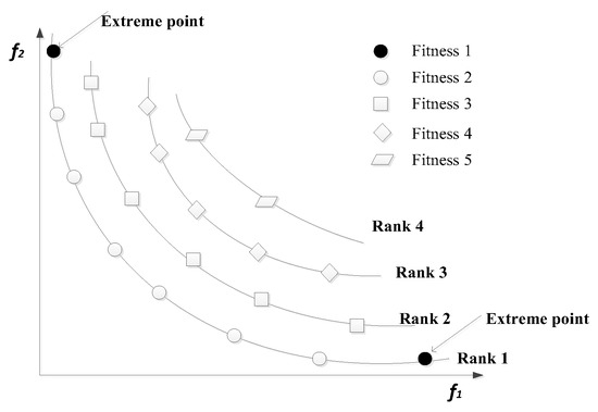
Figure 1.
Relationship between the non-domination rank and fitness.
Fitness value is calculated based on NS rank and their corresponding agent’s masses are determined given as below [26]:
where signifies the normalized mass, fitness value, worst fitness and best of agent at iteration.
3.3. Update the Agent’s Acceleration, Velocity, and Position
The agent’s acceleration in every repetition is computed as:
where, the constant of gravitational is at iteration, the gravitational constant is represented as , is specified constant, represents maximum iterations, is constant, indicates a Euclidean distance between two agents and at genearion, and is the best fitness value. The agent’s velocity and the position for the generation are calculated as below:
where indicates a random number between intervals [0–1], represent the velocity and position [33].
3.4. Moving Agents with Disruption Operator
The disruption operator is employed in the oppositional gravitational search algorithm (DOGSA) to avoid the algorithm from becoming locked in local optima and to improve local search [25]. The following criterion must be satisfied for disruption of the solutions:
The position of the solution satisfying the disruption criterion is updated as follows:
where is Euclidean distance between agents and is constant, is threshold value, indicates a random number among the intervals and is constant value.
Thereafter, the NS method in addition to the elite agent’s preservation is used for solving the multi-objective problems and fuzzy decision strategy implemented to obtain an optimal compromised result [32,33].
3.5. NSDOGSA Procedure for MSHTS Problem
The computational framework of the proposed NSDOGSA method for solving the MSHTS problem is shown in Figure 2 and described as follows:
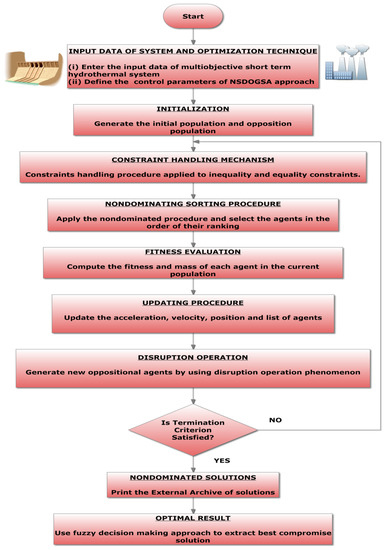
Figure 2.
Flowchart of NSDOGSA approach for MSHTS problems.
- Step 1:
- Enter the data from the hydrothermal test system and define the NSDOGSA’s settings. Create an opposition-based population by randomly initializing the water discharges and thermal power generation outputs for each agent in the population.
- Step 2:
- Constraint handling procedure is performed to satisfy end reservoir volumes and system load balance constraints.
- Step 3:
- Apply the NS strategy and update an external archive group.
- Step 4:
- Update the agent’s acceleration, velocity, and position.
- Step 5:
- Moving agent’s updating using disruption operator.
- Step 6:
- When prescribed iteration number is reached, stop the operation and store the trade-off solutions in an external archive; otherwise, go to Step 2.
- Step 7:
- Identify the non-dominated solution from the trade-off solutions by using a fuzzy decision strategy.
4. Discussion and Simulation Studies
NSDOGSA technique as well as other versions have been successfully used to address MSHTS issues on MATLAB 8.5 platform and prepared in PC (core i7-3rd Gen, 2.67 GHz, 8GB RAM). The suggested NSDOGSA approach is demonstrated on two MSHTS problems. The first one consists of 4 hydro and 3 thermal plants without considering transmission losses and another with the same system by including transmission losses. In order to study the feasibility and robust analysis of NSDOGSA, there are two standard test systems with different complex properties adopted from [22]. The complete hydraulic network and the complete hydrothermal information given in Appendix A. EPC and EEP functions are optimized separately by using DOGSA to enlighten the conflicting relation between these objective functions for MSHTS problems.
4.1. Test System-I
The parameters of the suggested approach have been obtained after fifty simulation runs. After fifty simulation runs, the parameters for NSDOGSA are given below: = 100, = 2000, = 20, = 0.5, = 150, = 15, and = 150. Additionally, the competency of the suggested methods are compared with the existing methods such as non-dominated sorting genetic algorithm (NSGA-II) in [19] multi-objective particle swarm optimization (MOPSO) in [22]. The size of the population, utmost generations, crossover and mutation probability of NSGA-II are 100, 2000, 0.45, and 0.2, respectively. MOPSO’s chosen parameters are as follows: swarm size = 100, maximum iterations = 2000, cognitive parameter = 4, social parameter = 3, and weight factor upper and lower values are 0.7 and 0.1, respectively.
The computational outcomes found by NSDOGSA for individual EPC, EEP, and MSHTS are mentioned in Table 1 and outperformed with other techniques such as SAGA [1], Fuzzy EP [2], MDE [3], DE [4], PSO [5], IQPSO [6], QPSO [7], QPSO-DM [7], QADEVT [8], PSO [9], PPO [9], PSO [10], PPO [10], PSO with PPS [10], PPO with PPS [10], SOHPSO-TVAC [11], HCRO-DE [12], CBIA [13], NPdynejDE [14], MODE-ACM [15], MODE [16], LM-MODE [16], CM-MODE [16], TM-MODE [16], MODE [17], CB-MOHDE [17], MOCA-PSO [18], NSGA-II [19], HMOCA [19], MOABC [20], NBIM [21], MODE-ACM [22], NSGA-II [22], MOQPSO [22], MODE [23], PMODE [23], NSPSO [28], NSPSO-CM [28], NSGSA [28], NSGSA-CM [28], GSA [29], IGSA [29], and IMOGSA [30].

Table 1.
Performance evaluation of different methods for MSHTS of Test system-I.
Table 2 and Table 3 show the rate of water discharges hourly and hydrothermal generation production values for the individual minimization of EPC and EEP using the DOGSA technique. Figure 3 depicts the graphical characteristics of EPC and EEP using the DOGSA method.
Table 2.
EPC minimization schedule results with DOGSA of Test System-I.
Table 3.
EEP minimization schedule results with DOGSA of Test system-I.
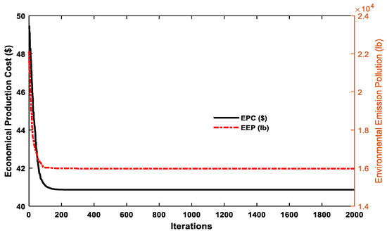
Figure 3.
Performance characteristics of EPC and EEP with DOGSA for MSHTS of Test System-I.
In MSHTS, the proposed NSDOGSA approach is optimized for both the EPC and EEP simultaneously, and obtained non-dominated solutions are shown in Table 4. The selection of feasible solutions among trade-off solutions is obtained with the help of a fuzzy decision-making approach. Figure 4 and Table 5 show the complete MSHTS schedule for the selected feasible solution.
Table 4.
Non-dominated solutions for MSHTS of Test System-I achieved using various methods.
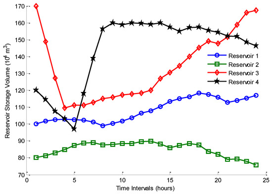
Figure 4.
Storage volume of reservoir with NSDOGSA for MSHTS of Test System-I.
Table 5.
Schedule results for the MSHTS of Test System-I should be compromised with NSDOGSA.
4.2. Test System-II
Test system-I with the transmission losses is considered to be Test system-II to impose more complexity, and also justify the robustness of the proposed NSDOGSA approach. To tune the parameters of NSDOGSA, 50 trial runs are performed, and thereafter the selected prime parameters for NSDOGSA are as follows: =100, =2000, =20, =0.5, =150, =15, and =150. The size of chromosomes, termination criteria, selection tournament, crossover parameter, and mutation value of probability for NSGA-II have all been set to 100, 2000, 0.7, and 0.4, respectively. MOPSO parameters are chosen as follows: swarm size = 100, maximum number of evolutions = 2000, cognitive constant = 7, social constant = 1.5, and maximum and minimum parameters of weight= 0.8 and 0.3. The computational outcomes found by NSDOGSA for separate EPC, EEP, and MSHTS are obtainable in Table 6 and analyzed with published techniques includes MDE [3], MODE [16], LM-MODE [16], CM-MODE [16], TM-MODE [16], MODE [17], CB-MOHDE [17], NSGA-II [18], MOCA-PSO [18], NSGA-II [19], HMOCA [19], MOABC [20], MODE-ACM [22], NSGA-II [22], MOQPSO [22], MODE [23], PMODE [23], HMOCA [30], NSGA-II [30], and IMOGSA [30] published in the literature.
Table 6.
Performance evaluation of Test System-II’s multiple approaches.
It is understood from Table 6 that the single EPC optimization: EPC is 42,738.57$ and EEP is 20,617.73 lb; for single EEP optimization: EPC is enlarged to 49,472.11$ and EEP is declined to 16,939.41 lb, and for MSHTS problem compromised with EPC is 43,664.12$ and 18,211.05 lb. Table 7 and Table 8 shows the optimal hydro water discharges and hydrothermal power outputs attained using DOGSA for separate optimization of EPC and EEP. The convergence characteristics for individual minimization of EPC and EEP with DOGSA approach are revealed in Figure 5.
Table 7.
EPC minimization schedule results with DOGSA for Test system-II.
Table 8.
EEP minimization schedule results of DOGSA for Test system-II.
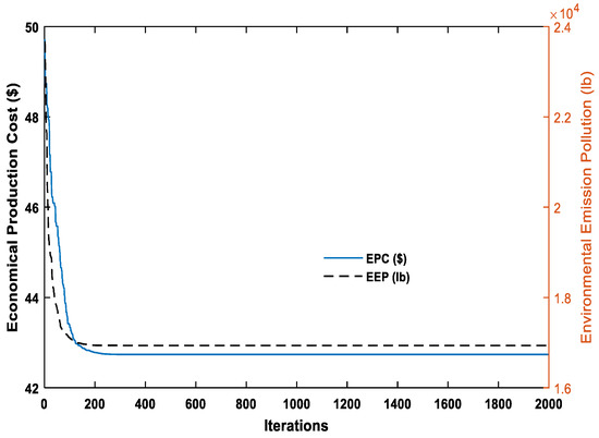
Figure 5.
Performance of convergence in EPC and EEP with DOGSA for MSHTS of Test system-II.
For MSHTS problem, the detailed objective function values of non-dominated solutions obtained with NSDOGSA approach are listed in Table 9. A fuzzy strategy is used to identify viable result from tradeoff solutions and corresponding optimal hydrothermal schedules are presented in Table 10 and Figure 6, which indicates the satisfaction of all kinds of constraints by using the constraints handling method.
Table 9.
NS results attained with various techniques for MSHTS of Test system-II.
Table 10.
Optimal MSHTS results with NSDOGSA for Test system-II.
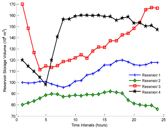
Figure 6.
Hydro reservoir storage volumes with NSDOGSA for MSHTS of Test system-II.
4.3. Statistical and Non-Parametric Analysis
Further, the statistical analysis is conducted to show the robustness of the proposed approach for separate minimization of EPC and EEP in terms of the best, average, worst, and standard deviation values, and for MSHTS problem with the highest cardinal priority ranking value which are presented in Table 11 and Table 12, for Test system-I and II.
Table 11.
Test System-I Statistical analysis with various approaches.
Table 12.
Test system-II Statistical analysis with various techniques.
From statistical analysis, it is clear that the superlative, middling, and wickedest objective values and standard deviation obtained with DOGSA after 50 runs are better than that obtained with GSA and its variants, which depicts the robustness of the solutions found with DOGSA approach. For MSHTS problem, the highest membership value obtained with the fuzzy decision approach is compared with NSGSA, NSOGSA, NSDGSA, and it is concluded that the NSDOGSA approach attains a greater satisfaction in terms of the quality of the solution. It can also be mentioned that the results obtained with the proposed approach show minimum standard deviation in values, which ensures the precision of the obtained results. To observe the robustness of the proposed algorithm for solving MSHTS problems, a well-known Kruskal–Wallis non-parametric test is conducted for all the test systems. It is a non-parametric method to test the null hypothesis that all the populations have the same median. This test can be used to compare three or more samples and assumed that the populations under comparison need not be normally distributed. Simulation results are obtained from 50 trial runs of the proposed algorithm and compared with the other methods for all the cases mentioned in box plots of Figure 7 for Test system-I and Figure 8 for Test system-II. It is observed that the probability of rejection of the null hypothesis is very low and variation is very small for the proposed method.
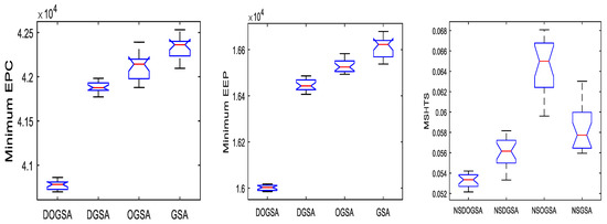
Figure 7.
Box-type plots of Kruskal–Wallis test for Test System-I.
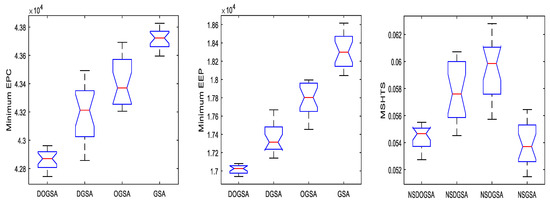
Figure 8.
Box-type plots of Kruskal-Wallis test for Test system-II.
5. Conclusions
In this paper, the hydrothermal scheduling problem is formulated in three different scenarios, namely: (a) minimizing economical production cost, (b) minimizing environmental emission pollution, and (c) minimizing both the objective functions while considering the water transport delay between hydraulic connected reservoirs, valve point loading effect of thermal units, and transmission line losses among generation units. The major contribution of the proposed work concludes that (i) an oppositional-based learning concept during the initiation phase and a disruption operator during the updating phase to achieve diversity and prevent premature convergence; (ii) the concept of a non-dominated sorting procedure has been presented to optimize both objective functions simultaneously to achieve a conflicting solutions in same computational run; (iii) an archive has been formed to store trade-off and a spread metric utilized to update the archive; (iv) a fuzzy strategy is adopted to select the best feasible solution; (v) an effective constraint approach has been formulated to satisfy the load balance and end reservoir storages; (vi) carried out on two MSHTS problems, the first one consisting of four hydro and three thermal plants without considering transmission losses, and another with including transmission losses results have been compared with the other existing approaches, and (vii) statistical analysis has been conducted to show the robustness of the proposed approach for separate minimization of EPC and EEP in terms of the best, average, worst, and standard deviation values, and for MSHTS problems with the highest ranking value, (viii) the simulation results with the proposed NSDOGSA revealed that it is an effective and competitive solution approach for solving complex MSHTS problems.
Further, the areas of the research and the solution techniques presented so far can be further extended to wider regions. In spite of all the above-mentioned contributions, much more intensive work still needs to be carried out, which can be broadly suggested for the following aspects such as (i) the work can be extended to consider the hydro and thermal unit commitment, which involves the optimization of continuous as well as discrete variables during the analysis, (ii) by considering additional complex constraints such as minimum up and down times of generating units, spinning reserve, ramp rates of thermal plants and prohibited zones of hydro plants, (iii) the scheduling problems can be further extended to consider the renewable energy such as tidal energy, wind energy, solar energy, etc., (iv) the present research work can be extended to include pumped storage plants for all scheduling problems, (v) the multi-objective optimization problems can also be handled using other aggregation methods such as ε-constraint method, normal boundary intersection method, lexicographic approach, etc., to generate non-dominated solutions.
Author Contributions
All of the authors contributed equally to this work such as conceptualization, G.N.; methodology, G.N.; software, H.P. and P.D.; validation, K.S.R.M.; formal analysis, P.S.V.; investigation, M.B.; resources, T.A.; data curation, W.E.-S.; writing—original draft preparation, M.M.F.; writing—review and editing, M.B. and T.A.; visualization, W.E.-S.; supervision, M.M.F.; project administration, M.B.; funding acquisition, P.S.V., M.B., T.A., W.E.-S. and M.M.F. All authors have read and agreed to the published version of the manuscript.
Funding
This work is funded by Researchers Supporting Project number (RSP2023R503), King Saud University, Riyadh, Saudi Arabia.
Acknowledgments
The authors appreciate Researchers Supporting Project number (RSP2023R503), King Saud University, Riyadh, Saudi Arabia.
Conflicts of Interest
The authors declare no conflict of interest.
Appendix A
Table A1.
Water discharge rate limits, reservoir storage volume limits, reservoir end storage conditions number of upstream plants, water transportation delays, and hydro plant generation limits (MW) for MSHTS of Test System-I and II.
Table A2.
Hydropower generation coefficients for Test System-I and II.
Table A3.
Reservoir inflows of Test System-I and II.
Table A4.
MSHTS problem Test System-I and II load demands.
Table A5.
Thermal generator data of Test System-I and II.

Figure A1.
Hydraulic network configuration for cascaded MSHTS of Test system-I and II.

References
- Basu, M. Goal-attainment method based on simulated annealing technique for economic-environmental dispatch of hydrothermal power systems with cascaded reservoirs. Electr. Power Compon. Syst. 2004, 32, 1269–1286. [Google Scholar] [CrossRef]
- Basu, M. An interactive fuzzy satisfying method based on evolutionary programming technique for multi-objective short-term hydrothermal scheduling. Electr. Power Syst. Res. 2004, 69, 277–285. [Google Scholar] [CrossRef]
- Lakshminarasimman, L.; Subramanian, S. Short-term scheduling of hydrothermal power system with cascaded reservoirs by using modified differential evolution. IET Gener. Transm. Distrib. 2006, 53, 693–700. [Google Scholar] [CrossRef]
- Mandal, K.K.; Chakraborty, N. Short-term combined economic emission scheduling of hydrothermal power systems with cascaded reservoirs using differential evolution. Energy Convers. Manag. 2009, 50, 97–104. [Google Scholar] [CrossRef]
- Mandal, K.K.; Chakraborty, N. Short-term combined economic emission scheduling of hydrothermal systems with cascaded reservoirs using particle swarm optimization technique. Appl. Soft Comput. 2011, 11, 1295–1302. [Google Scholar] [CrossRef]
- Sun, C.; Lu, S. Short-term combined economic emission hydrothermal scheduling using improved quantum-behaved particle swarm optimization. Expert Syst. Appl. 2010, 37, 4232–4241. [Google Scholar] [CrossRef]
- Lu, S.; Sun, C.; Lu, Z. An improved quantum-behaved particle swarm optimization method for short-term combined economic emission hydrothermal scheduling. Energy Convers. Manag. 2010, 51, 561–571. [Google Scholar] [CrossRef]
- Lu, S.; Sun, C. Quadratic approximation based differential evolution with valuable trade off approach for bi-objective short-term hydrothermal scheduling. Expert Syst. Appl. 2011, 38, 13950–13960. [Google Scholar] [CrossRef]
- Narang, N.; Dhillon, J.S.; Kothari, D.P. Multi-objective short-term hydrothermal generation scheduling using predator–prey optimization. Electr. Power Compon. Syst. 2012, 40, 1708–1730. [Google Scholar] [CrossRef]
- Narang, N.; Dhillon, J.S.; Kothari, D.P. Weight pattern evaluation for multiobjective hydrothermal generation scheduling using hybrid search technique. Electr. Power Energy Syst. 2014, 62, 665–678. [Google Scholar] [CrossRef]
- Mandal, K.K.; Chakraborty, N. Daily combined economic emission scheduling of hydrothermal systems with cascaded reservoirs using self-organizing hierarchical particle swarm optimization technique. Expert Syst. Appl. 2012, 39, 3438–3445. [Google Scholar] [CrossRef]
- Roy, P.K. Hybrid chemical reaction optimization approach for combined economic emission short-term hydrothermal scheduling. Electr. Power Compon. Syst. 2014, 42, 1647–1660. [Google Scholar] [CrossRef]
- Nguyena, T.T.; Dieu, V.N. An efficient cuckoo bird inspired meta-heuristic algorithm for short-term combined economic emission hydrothermal scheduling. Ain Shams Eng. Journal 2018, 9, 483–497. [Google Scholar] [CrossRef]
- Arnel, G.; Ales, Z. Short-term combined economic and emission hydrothermal optimization by surrogate differential evolution. Appl. Energy 2015, 141, 42–56. [Google Scholar]
- Qin, H.; Zhou, J.; Lu, Y.; Wang, Y.; Zhang, Y. Multi-objective differential evolution with adaptive Cauchy mutation for short-term multi-objective optimal hydro-thermal scheduling. Energy Convers. Manag. 2010, 51, 788–794. [Google Scholar] [CrossRef]
- Zhang, H.; Zhou, J.; Zhang, Y.; Fang, N.; Zhang, R. Short term hydrothermal scheduling using multi-objective differential evolution with three chaotic sequences. Electr. Power Energy Syst. 2013, 47, 85–99. [Google Scholar] [CrossRef]
- Zhang, H.; Zhou, J.; Zhang, Y.; Lu, Y.; Wang, Y. Culture belief based multi-objective hybrid differential evolutionary algorithm in short term hydrothermal scheduling. Energy Convers. Manag. 2013, 65, 173–184. [Google Scholar] [CrossRef]
- Rui, Z.; Zhou, J.; Wang, Y. Multi-objective optimization of hydrothermal energy system considering economic and environmental aspects. Electr. Power Energy Syst. 2012, 42, 384–395. [Google Scholar]
- Lu, Y.; Zhou, J.; Qin, H.; Wang, Y.; Zhang, Y. A hybrid multi-objective cultural algorithm for short-term environmental/economic hydrothermal scheduling. Energy Convers. Manag. 2011, 52, 2121–2134. [Google Scholar] [CrossRef]
- Zhou, J.; Liao, X.; Ouyang, S.; Zhang, R.; Zhang, Y. Multi-objective artificial bee colony algorithm for short-term scheduling of hydrothermal system. Electr. Power Energy Syst. 2014, 55, 542–553. [Google Scholar] [CrossRef]
- Ahmadi, A.; Kaymanesh, A.; Siano, P.; Janghorbani, M.; Nezhade, A.E.; Sarno, D. Evaluating the effectiveness of normal boundary intersection method for short-term environmental/economic hydrothermal self-scheduling. Electr. Power Syst. Res. 2015, 123, 192–204. [Google Scholar] [CrossRef]
- Zhong-kai, F.; Wen-jing, N.; Chun-tian, C. Multi-objective quantum-behaved particle swarm optimization for economic environmental hydrothermal energy system scheduling. Energy 2017, 131, 165–178. [Google Scholar] [CrossRef]
- Feng, Z.K.; Niu, W.J.; Zhou, J.Z.; Cheng, C.T.; Zhang, Y.C. Scheduling of short-term hydrothermal energy system by parallel multi-objective differential evolution. Appl. Soft Comput. 2017, 61, 58–71. [Google Scholar] [CrossRef]
- Rashedi, E.; Nezamabadi-pour, H.; Saryazdi, S. GSA: A gravitational search algorithm. Inf. Sci. 2009, 179, 2232–2248. [Google Scholar] [CrossRef]
- Gouthamkumar, N.; Sharma, V.; Naresh, R. Disruption based gravitational search algorithm for short term hydrothermal scheduling. Expert Syst. Appl. 2015, 42, 7000–7011. [Google Scholar] [CrossRef]
- Gouthamkumar, N.; Sharma, V.; Naresh, R. Hybridized gravitational search algorithm for short term hydrothermal scheduling. IETE J. Res. 2015, 62, 1–11. [Google Scholar] [CrossRef]
- Nobahari, H.; Nikusokhan, M.; Siarry, P.A. Multi objective gravitational search algorithm based on nondominated sorting. Int. J. Swarm Intell. Res. 2012, 3, 32–49. [Google Scholar] [CrossRef]
- Tian, H.; Yuan, X.; Ji, B.; Chen, Z. Multi-objective optimization of short-term hydrothermal scheduling using nondominated sorting gravitational search algorithm with chaotic mutation. Energy Convers. Manag. 2014, 81, 504–519. [Google Scholar] [CrossRef]
- Tian, H.; Yuan, X.; Huang, Y.; Wu, X. An improved gravitational search algorithm for solving short-term economic/environmental hydrothermal scheduling. Soft Comput. 2015, 19, 2783–2797. [Google Scholar] [CrossRef]
- Li, C.; Zhou, J.; Lu, P.; Wang, C. Short-term economic environmental hydrothermal scheduling using improved multi-objective gravitational search algorithm. Energy Convers. Manag. 2015, 89, 1227–1236. [Google Scholar] [CrossRef]
- Gouthamkumar, N.; Sharma, V.; Naresh, R. Nondominated sorting disruption based gravitational search algorithm with mutation scheme for multiobjective short term hydrothermal scheduling. Electr. Power Compon. Syst. 2016, 52, 1–15. [Google Scholar]
- Gouthamkumar, N.; Sharma, V.; Naresh, R. Application of nondominated sorting gravitational search algorithm with disruption operator for stochastic multiobjective short term hydrothermal scheduling. IET Gener. Transm. Distrib. 2016, 10, 862–872. [Google Scholar]
- Gouthamkumar, N.; Balusu, S.; Bathina, V. Nondominated sorting-based disruption in oppositional gravitational search algorithm for stochastic multiobjective short-term hydrothermal scheduling. Soft Comput. 2019, 23, 7229–7248. [Google Scholar]
- Coello, C.A.C.; Pulido, G.T.; Lechuga, M.S. Handling multiple objectives with particle swarm optimization. IEEE Trans. Evol. Comput. 2004, 8, 256–279. [Google Scholar] [CrossRef]
- Deb, K.; Amrit, P.; Sameer, A.; Meyarivan, T. A fast and elitist multi-objective genetic algorithm: NSGA-II. IEEE Trans. Evol. Comput. 2002, 6, 182–197. [Google Scholar] [CrossRef]
- Tizhoosh, H.R. Opposition-based learning: A new scheme for machine intelligence. In Proceedings of the International Conference on Computational Intelligence for Modelling, Control and Automation and International Conference on Intelligent Agents, Web Technologies and Internet Commerce, Vienna, Austria, 28–30 November 2005; pp. 695–701. [Google Scholar]
- Liu, H.; Ding, G.; Sun, H. An improved opposition-based disruption operator in gravitational search algorithm. In Proceedings of the 2012 Fifth International Symposium on Computational Intelligence and Design, Vienna, Austria, 28–29 October 2012; pp. 123–126. [Google Scholar]
- Marcel, F.; Lorca, Á.; Matías, N.P. Multistage adaptive robust optimization for the hydrothermal scheduling problem. Comput. Oper. Res. 2023, 150, 106051. [Google Scholar] [CrossRef]
- Sakthivel, V.P.; Thirumal, K.; Sathya, P.D. Quasi-oppositional turbulent water flow-based optimization for cascaded short term hydrothermal scheduling with valve-point effects and multiple fuels. Energy 2022, 251, 123905. [Google Scholar] [CrossRef]
- Paulo, V.L.; Renata, P.; Felipe, B.; Gabriel, T.; Erlon, C.F.; Lucas, B.P. Dealing with negative inflows in the long-term hydrothermal scheduling problem. Energies 2022, 15, 1115. [Google Scholar] [CrossRef]
- Saqib, A.; Muhammad, S.F.; Syed, A.R.K.; Ghulam, A.; Nasim, U.; Alsharef, M.; Mohamed, E.F. Introducing adaptive machine learning technique for solving short-term hydrothermal scheduling with prohibited discharge zones. Sustainability 2022, 14, 11673. [Google Scholar] [CrossRef]
- Muhammad, A.I.; Muhammad, S.F.; Noor, U.A.; Ahsen, T.; Irfan, A.K.; Ghulam, A.; Syed, A.R.K. A new fast deterministic economic dispatch method and statistical performance evaluation for the cascaded short-term hydrothermal scheduling problem. Sustainability 2023, 15, 1644. [Google Scholar] [CrossRef]
- Smarajit, G.; Manvir, K.; Suman, B.; Vinod, K. Hybrid ABC-BAT for solving short-term hydrothermal scheduling problems. Energies 2019, 12, 551. [Google Scholar] [CrossRef]
- Cui, Z.; Ali, T.H.; Ali, N.K.; Mingxin, J.; Muamer, N.M.; Nallapaneni, M.K. A rigid cuckoo search algorithm for solving short-term hydrothermal scheduling problem. Sustainability 2021, 13, 4277. [Google Scholar] [CrossRef]


Disclaimer/Publisher’s Note: The statements, opinions and data contained in all publications are solely those of the individual author(s) and contributor(s) and not of MDPI and/or the editor(s). MDPI and/or the editor(s) disclaim responsibility for any injury to people or property resulting from any ideas, methods, instructions or products referred to in the content. |
© 2023 by the authors. Licensee MDPI, Basel, Switzerland. This article is an open access article distributed under the terms and conditions of the Creative Commons Attribution (CC BY) license (https://creativecommons.org/licenses/by/4.0/).