Energy Performance of Occupant Behaviors on Windows: A Green Building Based Study

Abstract

In this paper, the window-opening behavior in a three-star green building with an operation mark in Ningbo was investigated. Four single offices facing south were selected, and the measurement lasted 20–40 days in the cooling season. An analysis of the relationship between window use and environmental factors was assessed by monitoring the occupancy state, the window action and window state, the time, and the temperature and humidity. A statistical analysis method was conducted to reveal the similarities and differences in window use among different occupants. The main findings were as follows: The window adjustment behaviors of different people vary significantly. In terms of adjustment time, there are two modes of behaviors. In addition, the occupancy state had a great impact on window action. Moreover, some people prefer to open the windows in the morning and close the windows at departure time, However, some of them prefer to open the windows at departure time and close the windows at the arrival time. Some irrational window opening behaviors were found in this research. Through correlation analysis, it was shown that the longer time the occupants were in the office, the higher window-opening duration and window-opening frequency would be. If the window was closed at arrival time, the total opening duration of window was significantly reduced. Also, window opening duration and closing duration are proportional to each other. With the help of principal component analysis (PCA) of the 12 features that affected window adjustment, the correlation between the window opening behaviors and the features could be clearly illustrated. A stochastic model of window-opening behavior based on logistics regression and uncertainty analysis was used in this paper. The cooling energy consumption of the stochastic model is 99.9% higher than the energy consumption generated by a fixed number of air changes, and the average energy consumption exceeds the fixed value by more than 21%. The findings of this study have certain guiding significance for promoting energy conservation by occupants’ behaviors in green buildings in this region.

1. Introduction

Green buildings and building energy-saving are important measures to reduce carbon emissions and environmental pollution [1]. For example, Madeeha Khan has found that integrating phase change materials (PCM) in building envelopes can greatly reduce building energy consumption [2]. Since different occupants behave variedly, which might result in large differences in energy consumption in two identical buildings [3] the implementation of green buildings not only requires efficient energy-saving technical measures [4], but also requires occupants to facilitate effects of energy-saving through reasonable behaviors [5]. Andersen, Olesen, and Jørn [6] found that different patterns of occupants’ behavior lead to up to 324% changes in energy consumption. The simulation by Clevenger and Haymaker [7] proposed that maximum energy consumption is 1.5 times higher than minimum energy consumption when different occupants’ behaviors are considered. Haldi et al. [8] found that occupants’ behavior (shade operation and window-opening behavior) has a significant impact on buildings’ energy demands. Tahmasebi, Farhang and Mahdavi et al. [9,10,11,12,13] improved the model of occupants’ presence and behavior with long-term monitored data from office areas, thereby enhancing the reliability of building performance simulations. It is, therefore, meaningful to understand and learn the characteristics of human behaviors. This would provide precise energy prediction [14] and analysis of building energy-saving effect in terms of various measures [15], and further promote behavioral energy saving [16].

Currently, the study on window adjustment in the research field of human behavior in buildings has received great attention. When the windows are open for ventilation, it will both decrease energy consumption [17] and improve thermal comfort [18]. Researchers have conducted actual measurement, modelling, and simulation analyses on window-opening behavior in different types of buildings [19,20,21,22].

For example, many studies have been conducted to investigate window opening behavior in different countries in Europe, such as the UK [23], Switzerland [21], Japan [24], Germany [19], Denmark [25], and Hungary [22]. Simultaneously, some Chinese researchers did tests on window opening behavior. After monitoring window states in 285 days, Pan [26] presented that occupants’ window-opening behavior is strongly affected by environmental factors, especially air temperatures. While the contextual factors also have an impact on the behavior. Similarly, window opening behavior in 19 residences in Beijing was studied by Yao et al. [27], and window behavior models were established through multivariate linear logistic regression. The research found that prioritization of the influence of environmental factors on window opening behavior. Shi et al. [28] reported some environmental factors have different effects on window-opening behavior in different seasons.

As these studies have different cultures and different climatic characteristics (most of them are located in the severely cold or cold regions [29]), leading to behavior differences of occupants [24], and the research conclusions are not suitable for the hot summer and cold winter zone of China. Although there have been some studies that researched window use in this region, they only focused on residential buildings [30,31] or hospitals [28]. The research about window uses in office buildings, especially green office buildings, still receive little attention. The actual performance of green building is closely relative to the occupants’ behavior. Therefore, understating the characteristic of window use in the green buildings will be of great importance in assessing the actual performance of green buildings. Additionally, most of the existing studies focus on the establishment of a window-opening behavior model of the whole person or average people [27,28,30].

However, there are significant differences in behaviors between different people [3]. Hence, the established model of average people might not well describe different behavioral characteristics [32] and their influences on energy consumption, if the diversity and similarity of behaviors among people are not clearly illustrated. Current studies lack analysis of behavioral differences among different people. For example, are there any significant differences between building energy efficiency professionals and ordinary people.

In this paper, the window use in a 3-star green building in the hot summer and cold winter zone of China was studied. The main objectives of this research are as follows:

(1) The different occupants’ behavioral characteristics of window use were analyzed through a statistical test method and, simultaneously, the correlation between any two relative behavioral factors were compared. Thus, the core characteristics of window use could be revealed;

(2) By analyzing the correlation between different people and behavioral characteristic parameters, comparing the similarities and differences between the behaviors of building energy efficiency professionals and ordinary people, and figuring out the irrational occupants’ behaviors in window use;

(3) Using a stochastic model of window opening behavior based on logistics regression to analyze the energy performance of occupants’ behaviors on windows and, therefore, the energy conservation by occupants’ behaviors in green buildings could be well promoted in green buildings.

2. Methodology

2.1. Case Building and Equipment Used

In this study, a 3-star green building based on China’s green building evaluation standard with four south-facing single offices was selected. The case building is located in Ningbo, one of the most important port cities on the southeast coast of China. The building was funded by the Global Environment Facility (GEF). The HVAC system adopts a ground-source heat pump system. The exterior window construction type is a heat-insulated metal profile window frame. SHGC (solar heat gain coefficient) is 0.54, gas tightness is 6, and visible light transmittance is 0.72. The area ratio of window to wall (WWR) facing east, south, and north is 0.35, 0.31, and 0.33, respectively. It belongs to the Cfa type in Köppen’s climate classification.

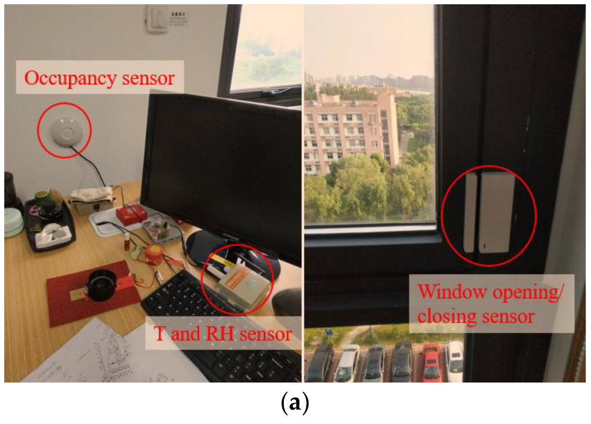
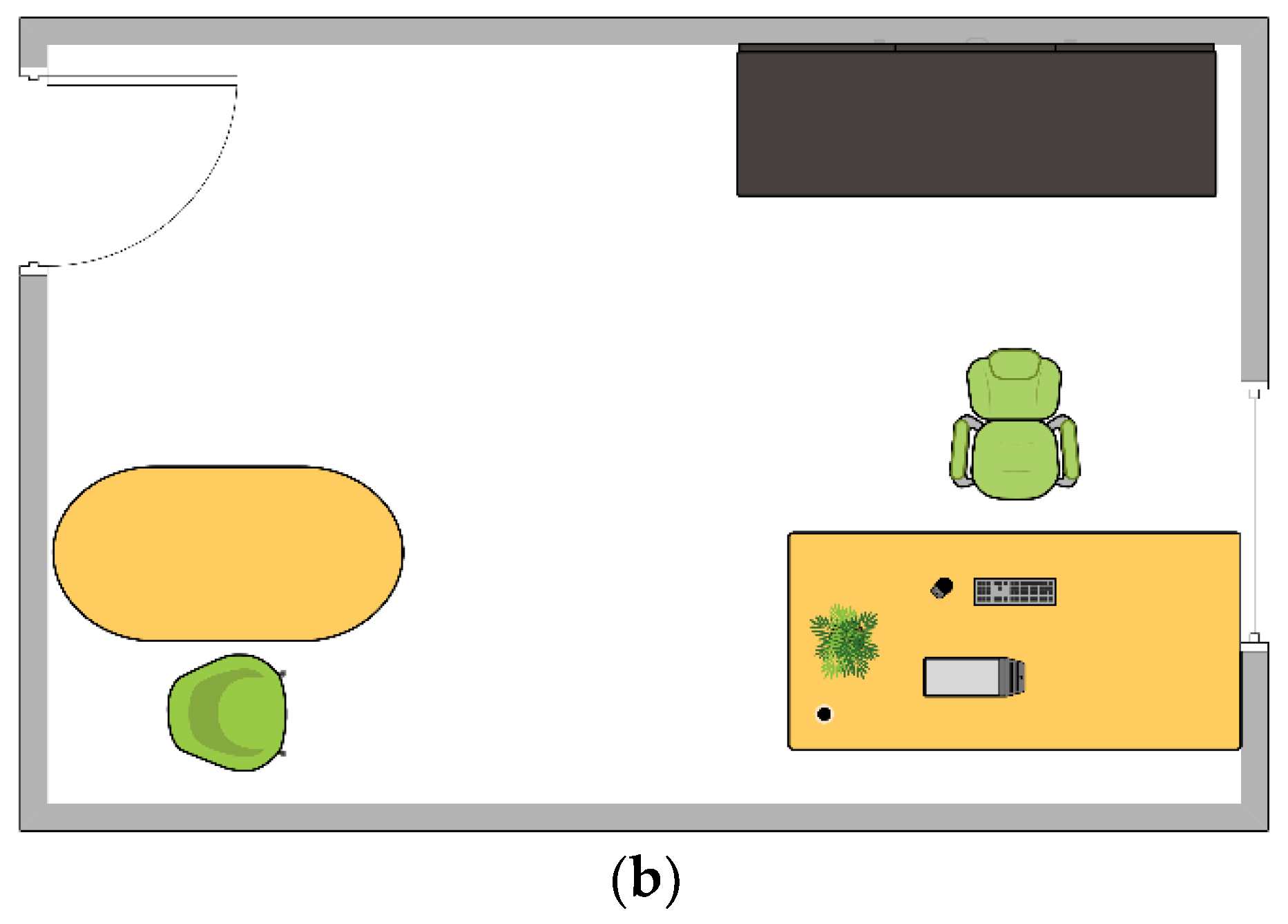
Two of these offices are on seventh floor and another two are located on the eighth and ninth floors, respectively. These offices have the same size, and the windows of each are in the same size, as well. The workstations are positioned so that the users’ line of sight is parallel to the window. Since window opening and closing behaviors could only be assessed under the conditions where people stay in the office, an occupancy sensor was installed in each office to detect whether there were people in the office [33,34]. Besides, as verified in previous studies, the temperature is the dominant factor leading to different window use [20,35,36], and Pan [37] suggested that occupants only sense the difference when CO₂ levels exceed 2000 ppm [24,38]. 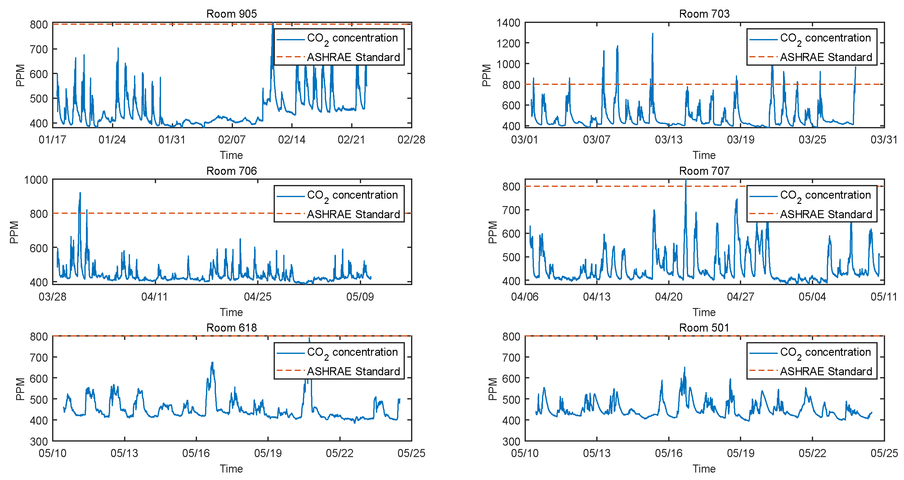Studies of the relationship between window-opening behavior and CO₂ concentration are presented in the Appendix A. Therefore, in order to analyze the potential parameters influencing window use, four variables, including indoor temperature, indoor humidity, outdoor temperature, and outdoor humidity, were selected. In addition to occupancy sensor, a temperature and relative humidity sensor and window opening/closing sensor were equipped, as shown in Figure 1a. As the wind speed and precipitation have not been measured, these two variables would not be taken into consideration. Four occupants taking part in the measurement were numbered from OCC-1 to -4. Sampling intervals were 1 min for occupancy state in order to capture the rapid dynamics of occupancy, and 5 min for indoor and outdoor temperature and humidity. Window state is incident-based, which means anytime when an opening or closing action appears, this action would be automatically recorded. The monitoring period ranged from 20 days to 40 days, and the total amount of days for the four occupants is 103 days (see

Table 1. Variables and durations.

ID	Indoor Variables	Outdoor Variables	Monitoring Period	Number of Days
OCC-1	Occupancy state (0 or 1, where 0 represents absent and 1 present); Window state (0 or 1, where 0 represents closed and 1 open); Air temperature, accuracy: 0.5 °C; RH, accuracy: 3%	Air temperature, accuracy: 0.5 °C; RH, accuracy: 3%	2/9/2019~22/9/2019	21
OCC-2			2/9/2019–11/10/2019	40
OCC-3			2/9/2019–21/9/2019	20
OCC-4			2/9/2019–23/9/2019	22

).

During the measurement period, the participants carried out their work normally, so behavioral characteristics of the window use could be truly reflected. The specific personnel characteristics are as follows: (1) OCC-1 is both an architectural designer and a teacher. (2) both OCC-3 and OCC-4 are architectural designers. (3) OCC-2 is an HVAC engineer and a professional engaged in building energy efficiency. OCC-2 has more knowledge of building energy-saving than others. Therefore, by comparing OCC-2 with others, we can understand whether there is a difference between building energy efficiency professionals and ordinary people in terms of energy saving through window use.

2.2. Statistical Test

To investigate the correlation among the variables, the Pearson correlation coefficient was applied to examine correlations between any two of the adjustment behavioral characteristics. In order to compare the behavioral characteristics of different people, a statistical comparison based on the Poisson distribution was used to compare the differences between building energy conservation experts and other people. Furthermore, since the Fisher exact test is more suitable for the case where the number of sample (n) is less than 40 or theoretical frequency (T) is smaller than 1, compared with the Chi-square test, such a test was conducted to compare the frequency of window use in different time periods.

2.3. Features of Window Use Behaviors

Since the measurement variables mentioned in Table 1 were based on different time intervals, for convenience, all the data were unified into a 5 min interval step size, which was consistent with the selected step size in other studies [39]. In order to analyze the occupants’ window use behaviors, investigate the interrelationship between behavior features, and further reveal the characteristics of adjustment behaviors, 12 features closely relative to the window opening behaviors were selected. These 12 features include daily average occupancy rate (based on 8 h working hours per day, excluding weekends and holidays), the ratio of total window opening time in the measurement period, the ratio of the total window opening time in the room’s occupancy time, the average daily frequency of window opening, average daily window opening frequency at arrival time, average daily window closing frequency at arrival time, average daily window opening frequency at departure time, average daily window closing frequency at departure time, average daily window opening frequency at intermediate period, average daily window closing frequency at intermediate period, the ratio of the average window opening time to 72 h duration, and the ratio of the average window closing time to 72 h duration. As the average window opening and closing time are in a different scale with other features, the ratio of these two durations to 72 h should be considered here to better show all the features in the same figure. The whole day would be divided into three periods, arrival (within 15 min from the time the first occupant arrived), intermediate and departure (within 15 min from the time the last occupant left), since previous studies have found that the probabilities of window action are higher at arrival time and departure time [19,40].

2.4. Principal Component Analysis

Principal component analysis (PCA) is used to summarize and to visualize the information in a data set described by multiple inter-correlated variables (in this paper, they are features related to window actions). The goal of PCA is to extract important information from the data and identify correlations in different data points. And two occupants have similar behavior patterns if they have similar values for all the 12 features, that is, if the Euclidean distance d defined by Equation (1) is small [41].

$$d\left(OC{C}_i,OC{C}_j\right)=\sqrt{{{\displaystyle \sum }}_k^{n=12}{\left(OC{C}_{i,k}-OC{C}_{j,k}\right)}^2}$$

(1)

The goal of PCA in this research is to identify the relationship between features and similarities between the four occupants, and to reveal the behavior features of each occupant, which is difficult to achieve by correlation analysis alone.

2.5. Regression Model

In order to further explore the window opening behavior, and the influence of environment and time, the five variables, including window use, durations, indoor temperature and relative humidity, and outdoor temperature and humidity, were input for multivariate linear logistic regression. As window use proceeds when occupants stay at the offices, only the time when the room was occupied was considered. The equation of the logistic regression is shown as Equation (2).

$$logitP=\log \left(\frac{P}{1-P}\right)={\beta }_0+{\beta }_1{x}_1+\cdots +{\beta }_n{x}_n$$

(2)

Equation (2) could be further developed into Equation (3).

$$P=\frac{1}{1+e^{-\left({\beta }_0+{\beta }_1{x}_1+\cdots +{\beta }_n{x}_n\right)}}$$

(3)

where, P is the probability of window adjustment, x is the factor that affects the opening and closing of the window, and beta is the coefficient of the regression equation. To determine which of these five variables have an impact on occupants’ behaviors, a stepwise regression method was used. The input variables for the model were ensured by Akaike Information Criterion (AIC). In research, AIC is used to compare different possible models and determine which one is best for the given data. The smaller values of AIC represent the better models.

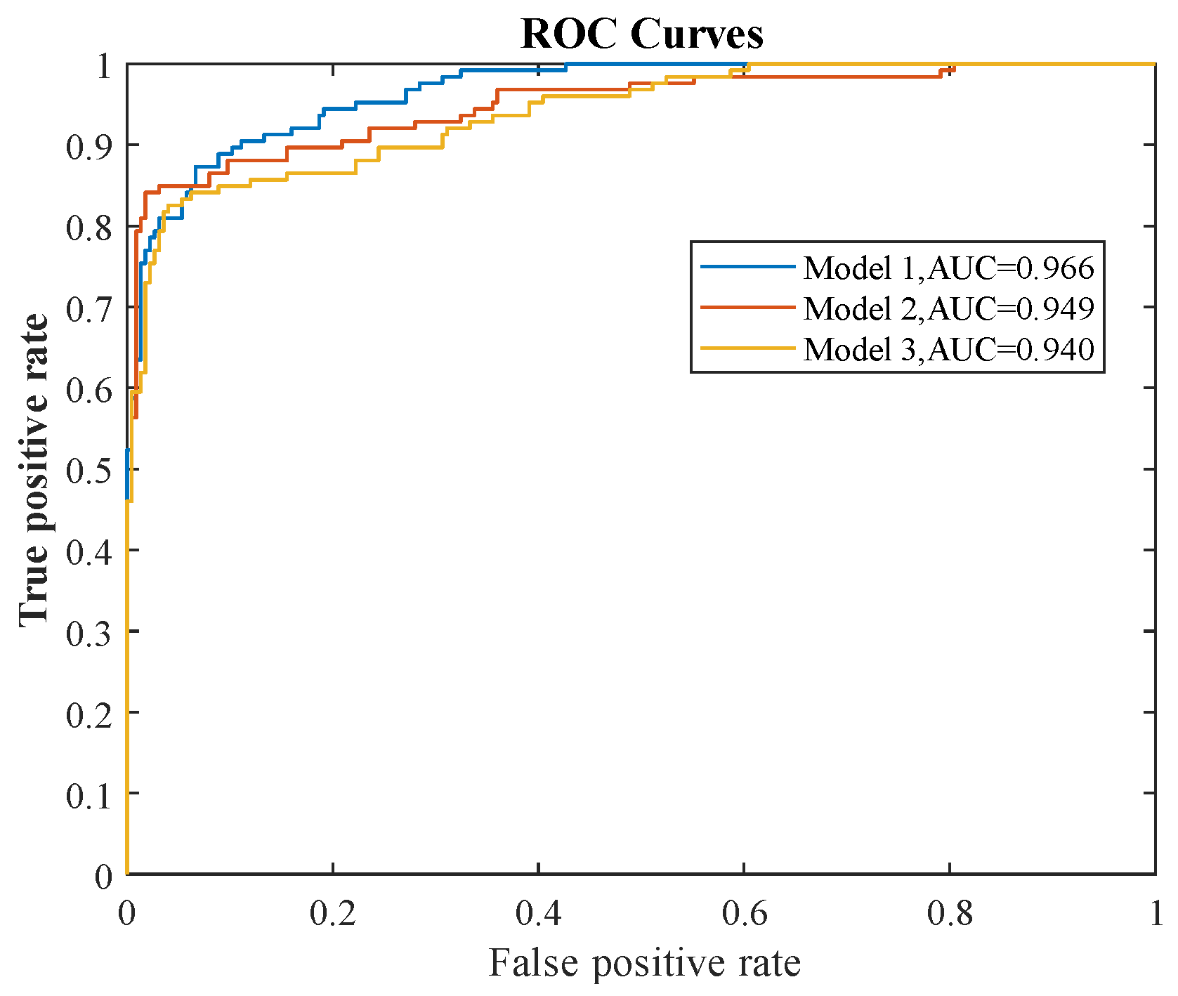
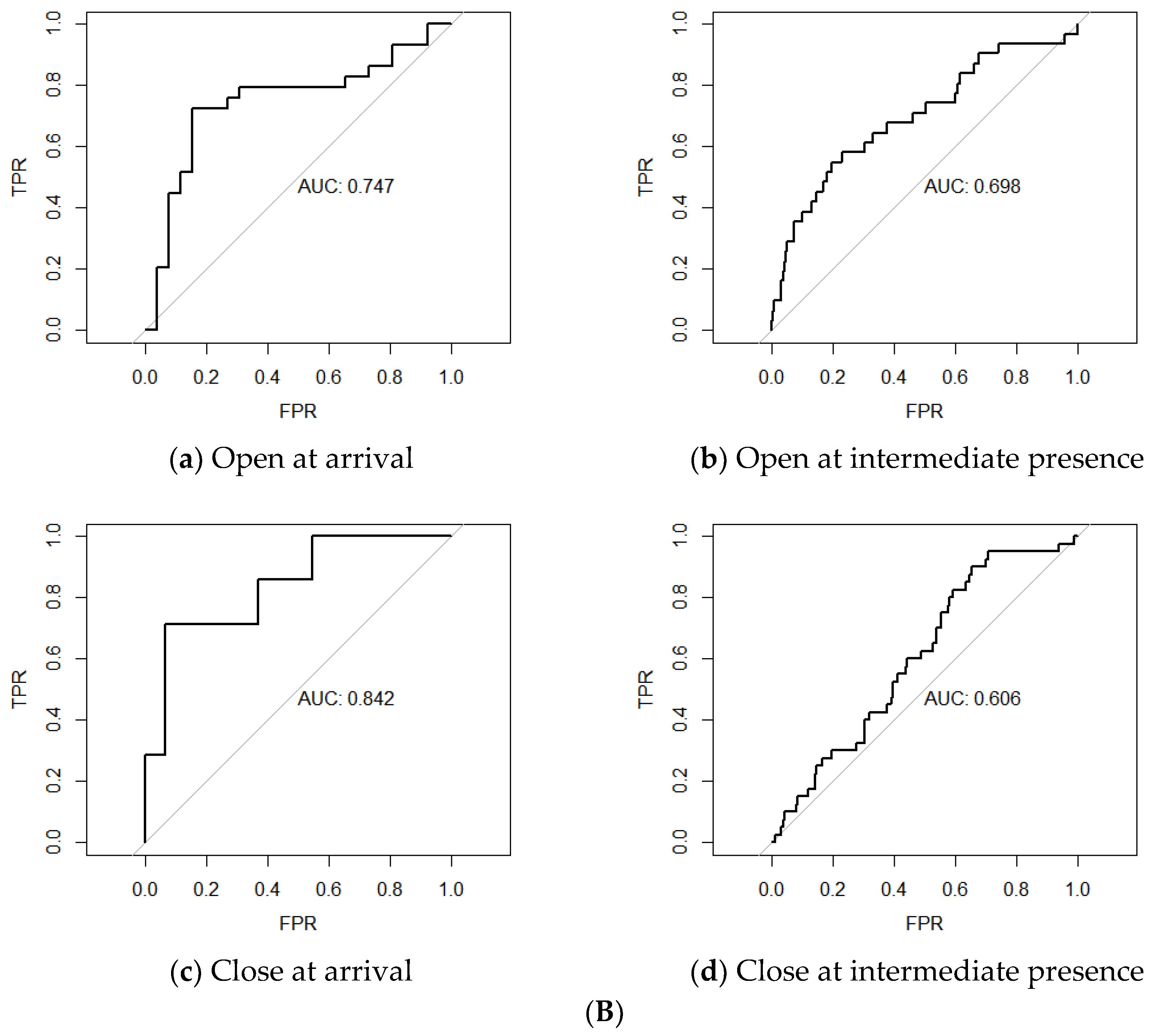
In order to analyze the probability of window adjustment in different periods, the time periods in terms of arrival to the office, intermediate, and departure from the office were chosen. In addition, the ROC curve could also be obtained through the regression model. The ROC curve greatly illustrates the prediction accuracy of the logistic regression. A case introduction of ROC is provided in Appendix A (including example).

2.6. Energy Consumption Simulation

A typical office building with a fixed number of air changes per hour for the infiltration and the stochastic model of occupants’ behavior was used in this paper. The stochastic model has the same schedule as reality, and the window-opening behavior is controlled by Energy Management System (EMS) of Energyplus.

For uncertainty analysis of natural ventilation, the number of repeated simulations required was first determined to get a converged result. Correlation analysis is then performed to verify the randomness between each simulation. The Kolmogorov–Smirnov test and the Shapiro–Wilk test were used to ensure that the energy consumption data conformed to a normal distribution. By comparing the total energy consumption of buildings generated by the fixed number of air changes per hour for the infiltration and the stochastic model of window-opening behavior, the influence of occupants’ behavior on building energy consumption can be explored. Based on the comparative results, effective suggestions can be provided for the operation and management of other green buildings in the region [42].

Considering that the experimental monitoring period is summer, according to «Design standard for energy efficiency of public buildings GB50189-2015» [43], the simulation date was set from 15 June to 31 August. The number of air changes per hour for the infiltration amount was determined to be 0.833 as shown in Equation (4).

$$AirChanges=\frac{zone population\times fresh air requirement}{Room volume}$$

(4)

AirChanges is the number of air changes per hour for the infiltration amount. Zone population is the number of people in the ventilation zone during typical usage. fresh air requirement is fresh air requirement per person.

Occupants’ behavior on windows is random, which leads to great uncertainty in building energy performance. In order to obtain a large number of random energy consumption data, 50 co-simulation runs were conducted and the timestep is set to 10 min.

A south-facing office room (8.4 × 4.2 × 3.6 m) of the case building was used in this study. The size of the window is 1.5 × 2.1 m. As shown in

Table 2. Characteristics of simulation settings.

Parameter	Value
Location	Hangzhou city in China, latitude: 30° N, longitude: 120° E
Orientation	South
Run period	15 June to 31 August
Dimension	Room: 8.4 × 4.2 × 3.6 m, Window: 1.5 × 2.1 m (WWR: 0.208)
Building envelope	U-value for external wall:0.5 W/m2K; U-value for roof:0.39 W/m2K, U-value for floor:0.46 W/m2K, Window setting: Painted Wooden window frame (U-value: 3.633 W/m2 K); Glazing type: Project external glazing (U-value: 1.96 W/m2K)
Work schedule	8:00–17:00 for weekdays during the summer
HVAC	Office Cooling Setpoints: 23.9 °C, run time: 5:00–19:00
Interior heat generation	Light density:5 W/m2
Mechanical ventilation	Run time: for weekdays Summer Designday, 8:00–19:00

, the simulation model setting complies with the real condition in this region.

3. Result and Discussion

3.1. Statistical Test Results

3.1.1. Frequency of Actions

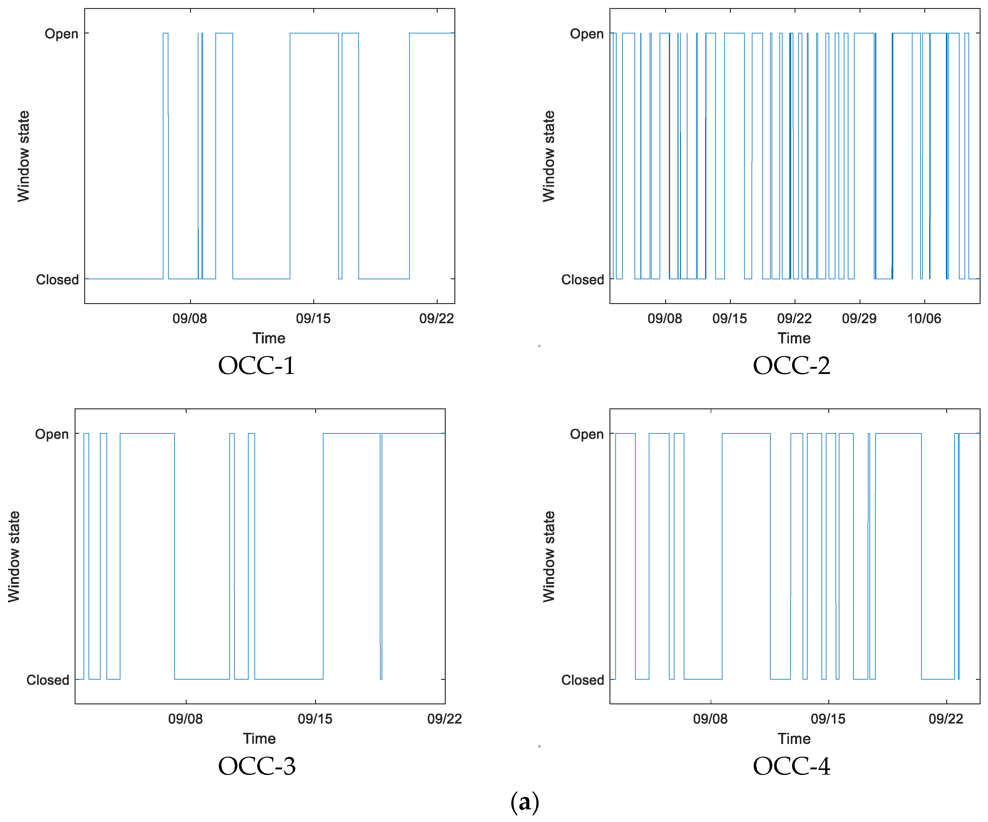
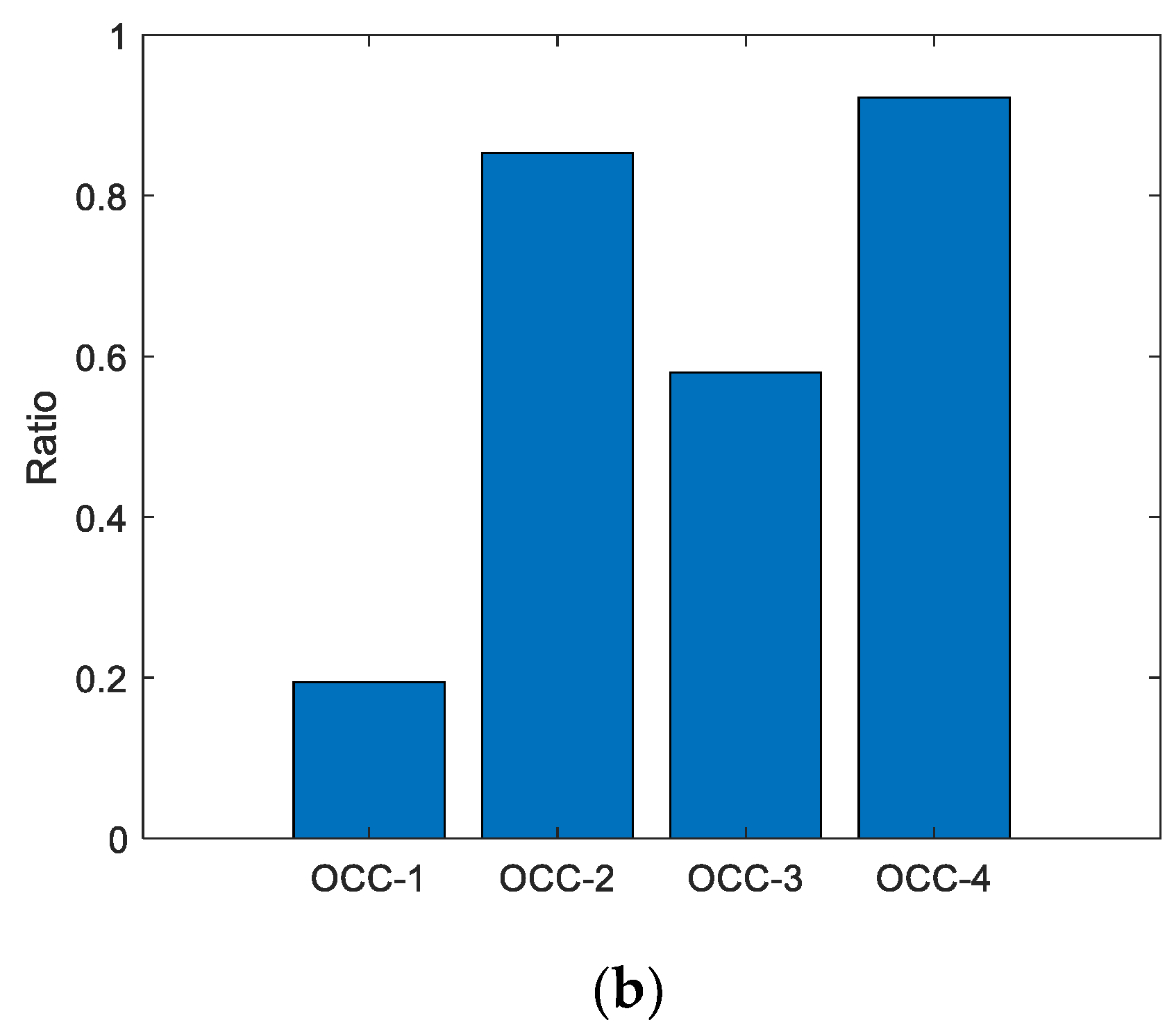
Figure 2a indicates the frequency of window-opening behaviors for the four participants. The measurement duration for OCC-2 is 40 days, whereas that for the other three is around 22 days. In terms of the action frequency, OCC-2 has a higher value than others. The daily average opening frequency for each one was calculated, and the results show that OCC-2 has the highest value of 0.92, followed by OCC-4 (0.54), OCC-1 (0.38) and OCC-3 (0.35). Therefore, they could be divided into three categories as high frequency, mid frequency, and low frequency for window opening. In order to compare the results from the statistical perspective, the daily window opening frequencies were compared by changing the survey durations of all four participants to 40 days, meaning that the frequency for OCC-1 n₁ is 15.24, the frequency for OCC-2 n₂ is 37, the frequency for OCC-3 n₃ is 14, and the frequency for OCC-4 n₄ is 21.81. If the difference between n₂ and the other three values is not evident, then n₁, n₂, n₃, and n₄ obey the same Poisson Distribution, and the calculation results for $\frac{n_2-n_i}{\sqrt{n_2+n_i}},i=1,3,4$ are in line with the Normal Distribution with a mean of 0 and a variance of 1 [44]. In other words, the calculation result of $\frac{n_2-n_i}{\sqrt{n_2+n_i}}$ will lie between [−1.96 and 1.96] under the probability of 95%. However, the actual calculated results show that the values of OCC-2 and the other three are −3.02, 3.23, and 1.98, respectively, which are all outside the range. This shows that there is a 95% probability that the number of adjustments for OCC-2 is significantly higher than that of the other three. That is to say, there is a huge gap in the frequency of window opening between people who know more about building energy efficiency and the others.

Furthermore, the frequency of adjustment and daily average occupancy rate (demonstrated in Figure 2b, determined by taking 8 working hours per day and ignoring weekends and holidays) was also compared. It is found that the occupancy rate for both OCC-4 and OCC-2 are high, which is related to the high frequencies of window opening. The occupancy rates for OCC-1 and OCC-3 are low, especially for OCC-1, as OCC-1 is always outside the room for teaching in the school. Therefore, the frequencies for window opening for these two people are also relatively low.

3.1.2. Time of Actions

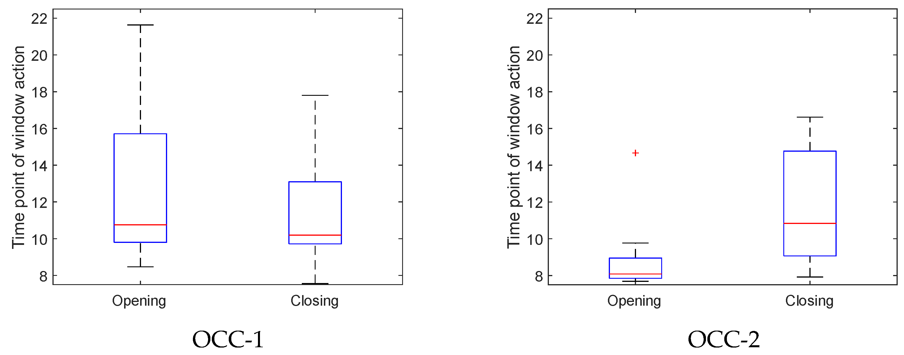
Figure 3 describes the time at which window was opened and closed for the four participants. It shows that there are two kinds of behaviors: the first one is opening the window in the morning and closing it in the afternoon (OCC-2 and OCC-3), which is in line with the former studies [19,40]; the other one is closing the window before opening it (OCC-1 and OCC-4). OCC-1’s behavior might be related to his work. Since OCC-1 always goes to teach in the school, his behavior is not similar with the common one. OCC-4’s behavior might be related to his personal preference (known from the conversation), which also has a significant impact on window opening action [26].

3.1.3. Duration of Window States

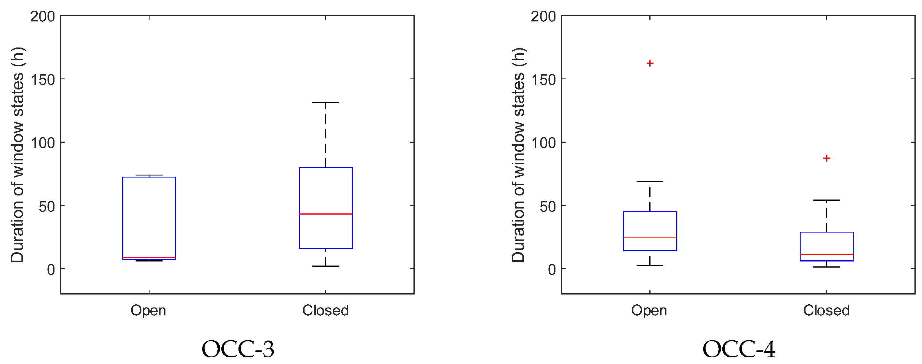
Figure 4 shows that there are huge uncertainties in the duration of window opening and closing. The shortest window opening only lasts dozens of minutes, while the longest window opening duration reaches more than 100 h (about 4–5 days). The longest window opening duration of OCC-3 is more than 350 h, which is equivalent to half a month. The average window opening and closing durations of OCC-1 is 23.9 h and 34.8 h, respectively, the values of OCC-2 is 13.2 h and 14.6 h, respectively, the values of OCC-3 is 68.8 h and 51.4 h, and that of OCC-4 is 37.3 h and 22.0 h, respectively. It can be seen that the opening and closing time of OCC-2 is the shortest—only half a day. This is due to its higher adjustment frequency according to the analysis above. Also, according to the opening and closing time mentioned before, it can be seen that OCC-2 usually opened the window in the morning and closed it in the afternoon. The window opening and closing durations of OCC-3 are the longest, about 4–5 times longer than that of OCC-2. The durations of the other two participants are relatively close, both are within the range of 20–30 h. The main difference between the two is that the window closing time of OCC-1 is longer than that of window opening, whereas the situation of OCC-4 is in contrast.

Previous studies [20] show only 25% and 50% of residential windows are left open at night. However, in this study, it is found that the window closing rate at nights for the four participants are 21.84%, 19.5%, 17.93%, and 11.76%, respectively, which are relatively low. This phenomenon may be led by the action of strengthening the natural ventilation at night, but this needs to be testified in the future.

3.1.4. Number of Actions

Previous studies have shown that windows were often opened when people first arrived at the office in the morning, and they were usually closed when people left the office after getting off work. Therefore, in order to better analyze the time distribution at which the window was opened and closed, and to understand whether these four people had such behavior, Figure 5a classifies the time in terms of arrival to the office, intermediate, and departure from the office. According to Figure 5a, the times at which the window was opened and closed of OCC-1 are relatively close, whereas that for the other three have some differences.

For quantitative comparison, the Fisher Test method is used, which has an advantage over the Chi-Square Test because it can analyze small samples whose frequency is less than 5, and most of the values in this study are less than 5. The test results show that the p-values for the four are 0.8135, 0.0007607, 0.3718, and 0.03607, respectively. Therefore, according to the threshold of significance p = 0.05, there is a significant gap between the adjustment frequency of the window opening and closing of OCC-2 and that of OCC-4 in different time periods, whereas the other two have no significant difference. The difference between OCC-2 an OCC-4 is that OCC-2 often opened the window in the morning and closed it in the afternoon and evening, whereas OCC-4 usually closed the window in the intermediate period and opened the window when leaving. In addition, to summarize the results of all four participants, Figure 5b can be obtained as follows. The p-value is gained as 0.0006525 by using the Fisher Test. It shows that there is a significant difference. From Figure 5b, it is seen that window opening behavior often occurs in the morning and intermediate period, whereas window closing behavior often occurs in intermediate time and the evening. Therefore, if the average person model which is considered in most previous studies is adopted, the behavior of people like OCC-4 cannot be reflected.

3.2. Analysis of Irrational Window-Opening Behavior

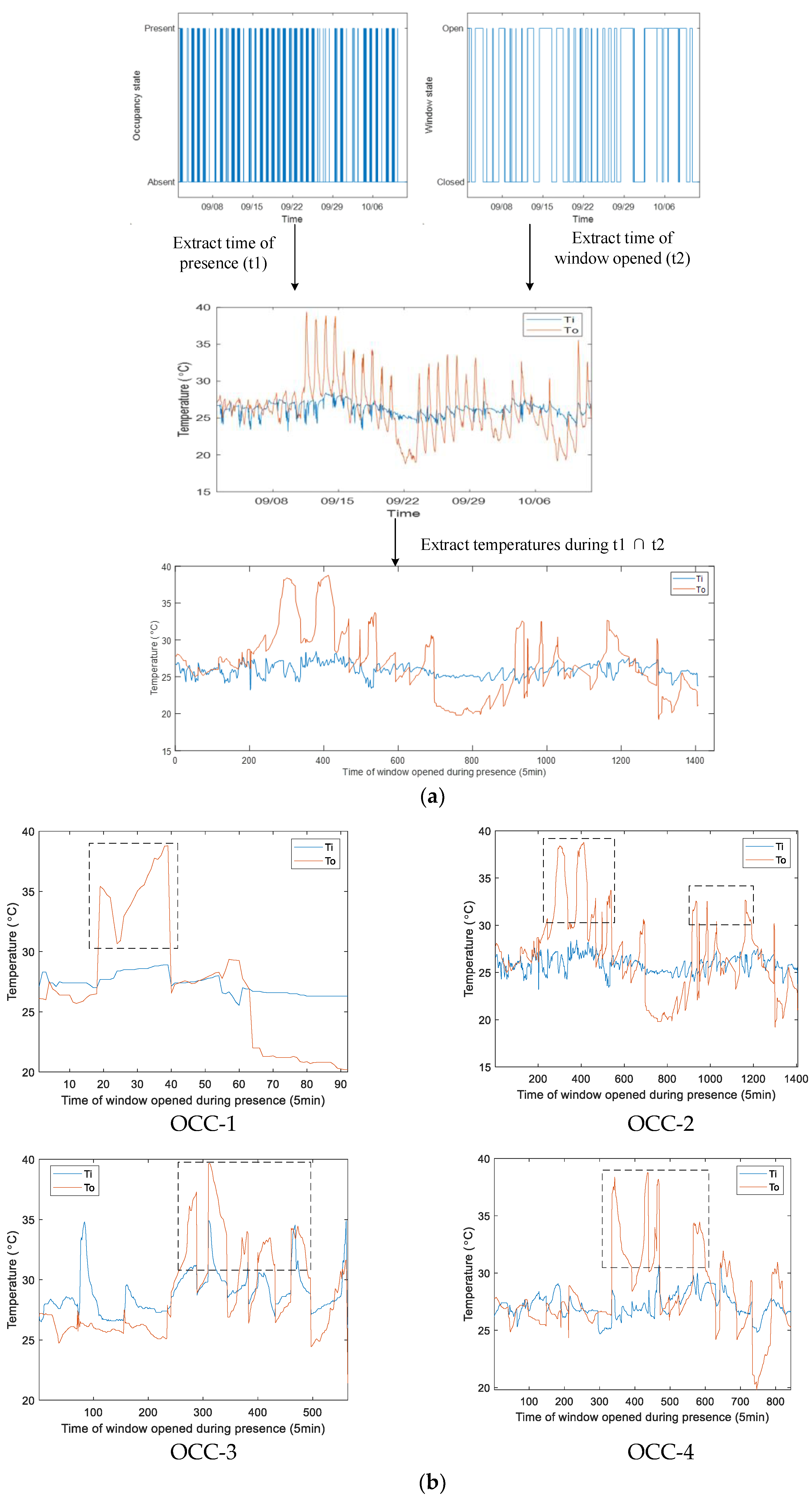
The irrationality of window action is analyzed by using the method shown in Figure 6a. The duration people stay in the room and that of window opening intersected so that the duration for the window opening when people are in the room can be presented. Next, the outdoor air temperature for this period was obtained. In this study, it is assumed that it is irrational if the window was opened when the outdoor air temperature was above 30 °C, as it would increase the heat gains and the consequent cooling demand. Figure 6b shows the temperature variation within this period and it can be concluded that all four participants demonstrated irrationality for window opening. The part of the temperature curve in the dash boxes exceeds 30 °C and it peaks at 35 °C. Meanwhile, it can also be observed that the air conditioning was on during the period corresponding to these boxes. Therefore, there is an irrational behavior of using air conditioners and windows simultaneously for all four participants.

Moreover, the ratio of this irrationality was quantified based on the ratio of the duration of window opening when the outside air temperature is above 30 °C and the testing duration. The ratios of the four were obtained as 6.7%, 7.1%, 8.1%, and 8.8%, respectively, which are relatively close. Thus, the rationality for window opening of the building energy efficiency professional is not higher than the others.

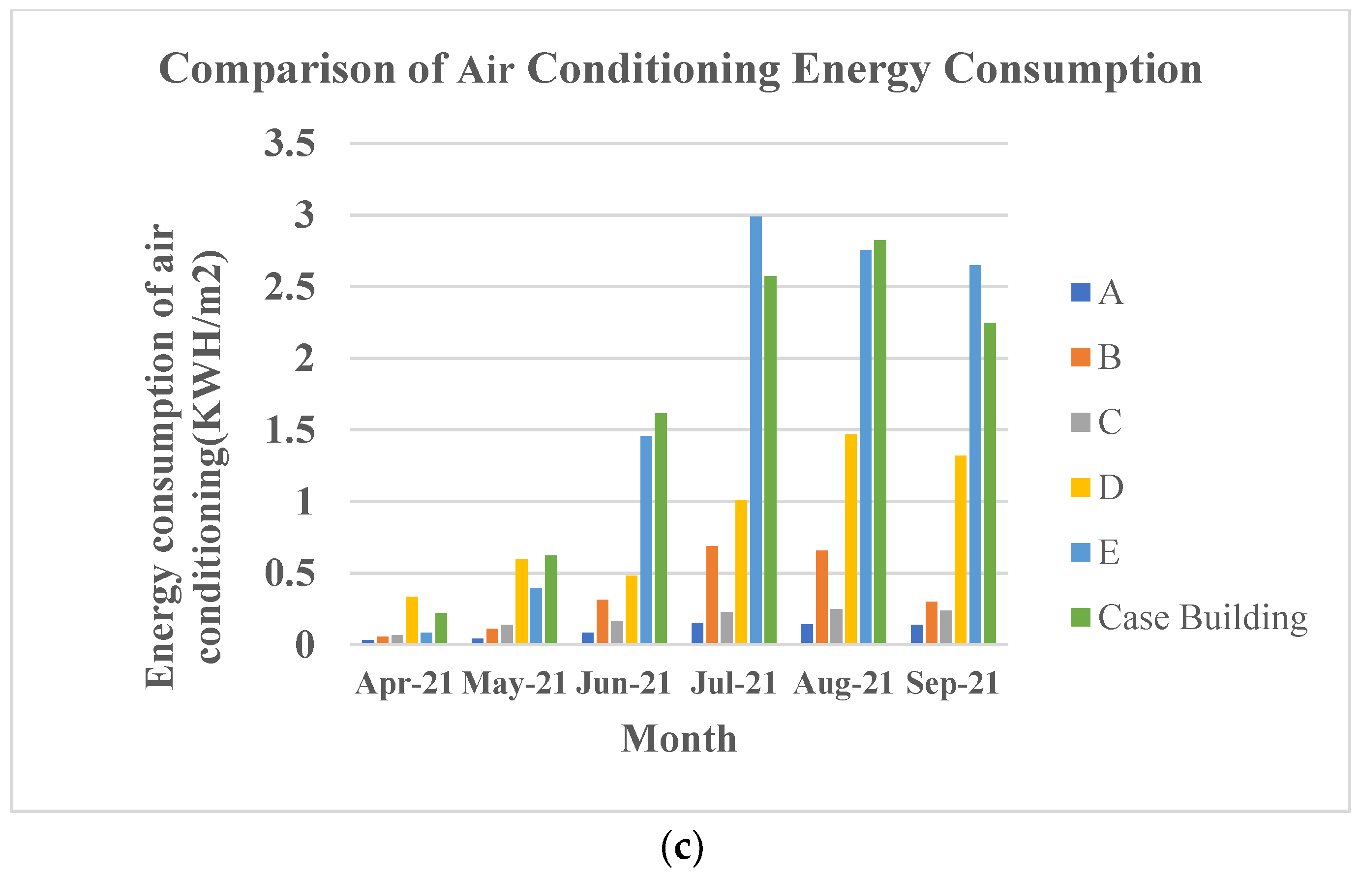
In order to analyze the energy consumption of this building, we established the Energy Consumption Monitoring Platform to monitor the energy consumption of most buildings in real time. Using the platform data, Figure 6c shows the air-conditioning energy consumption per unit area of the office building during the experiment period, and it is found that the energy consumption of the case building ranks among the top for the same type of buildings.

The results show that irrational behaviors (windows were left opened for long periods even when air-conditioning was switched on) may lead to high energy consumption in green buildings. Since green buildings have taken energy-saving technologies, the energy-saving effect of the building envelope and the HVAC equipment is outstanding, and occupants’ behaviors (window-opening behaviors) has a greater impact on energy consumption. Therefore, the improvement of irrational behaviors contributes to reducing building energy consumption, and it is necessary to improve occupants’ behaviors.

3.3. Analysis of Behavioral Characteristics

Figure 7a indicates the comparison of the 12 features for the window opening behaviors of the four participants.

Table 3. The 12 features for window opening behavior.

12 Features	OCC-1	OCC-2	OCC-3	OCC-4
Duration-close-72 h	0.48	0.20	0.71	0.31
Duration-open-72 h	0.33	0.18	0.96	0.52
Wclose-inter-daily	0.14	0.63	0.15	0.41
Wopen-inter-daily	0.10	0.39	0.2	0.18
Wclose-dep-daily	0.12	0.18	0.13	0.10
Wopen-dep-daily	0.12	0.08	0	0.38
Wclose-arr-daily	0.12	0.10	0.06	0
Wopen-arr-daily	0.24	0.49	0.17	0
Wopen-daily	0.38	0.93	0.35	0.55
Wopen-occ	0.33	0.66	0.68	0.60
Wopen-all	0.36	0.50	0.53	0.60
Occupancy	0.19	0.85	0.58	0.92

shows values for the 12 features for window-opening behavior. It shows that the ratios of the common behavior of opening the window at arrival time and closing the window at departure time are not high. The highest ratio for opening the window when getting to work is only 50%, and the average value is only around 30%. The highest ratio for closing the window when getting off work is only 20%, and the lowest value is around 10%. Both average values are significantly lower than that reported by other studies as 63% and 60%, respectively [36]. In other words, the window opening behaviors of the four are different from those in other districts—they are not used to opening window when getting to work and closing it when getting off work. In contrast, their ratio of opening or/and closing window in the intermediate time is relatively higher. In addition, the ratio of the total window opening time to the total testing time is basically the same as the ratio of the total window opening time to the room’s occupancy time, indicating that the presence or absence of a person in the room does not have a significant impact on the ratio of the window’s open time to the closed time. This implies that it may not be useful to increase the ratio of window opening to strengthen natural ventilation by increasing the occupancy rate of the room.

In order to understand the relationship between the behavioral characteristics, the correlation coefficient between these factors was calculated. Figure 7b provides the Pearson Coefficient of these elements, and 1 stands for the complete positive and –1 represents the complete negative. The bigger the circle is, the stronger the relationship. Furthermore, the correlation coefficients are also provided inside the circle. Blue means positive and red means negative. The following critical questions regarding to window opening and closing can be answered by analyzing the correlation.

(1)

Which characteristics of window opening/closing are affected by the occupancy rate?

Figure 7b shows that the occupancy rate is closely related to the ratio of the total window opening time (0.89), and it is also positive to the average daily window opening frequency at the intermediate period (0.67) and average daily window closing frequency at the intermediate period (0.78). This indicates that if the occupancy rate is higher, the total window opening duration and the frequencies of window opening and closing when the room is occupied will be higher. Moreover, the occupancy rate is not related to the behavior of opening the window when getting to work, closing the window when getting off work, and the duration for each window opening. It means that higher occupancy rate will not increase the average window opening time. Nevertheless, the correlation between the occupancy rate and the average window closing time was found to be negative, meaning that higher occupancy rate would lead to lower duration for window closing. This might be due to the fact that when the occupancy rate is higher, the frequency for window opening and closing would increase, so the duration for each window opening and closing action would remain the same.

(2)

What is the relationship between the window opening and closing frequencies?

It shows that the strongest correlation occurs between the average daily window opening frequency (Wopen.daily) and average daily window closing frequency in the intermediate period (Wclose.inter.daily) with a correlation coefficient of 0.97. Furthermore, the former feature is also strongly related to the average daily window opening frequency at intermediate period (the coefficient is 0.9). This indicates that higher daily window opening frequency would result in higher frequency of daily window opening when the room is occupied. In addition, the relation between average daily window opening frequency at arrival time and average daily window closing frequency at departure time is also strong (the coefficient is 0.95). Moreover, the ratio of total window opening time in the measurement period is found to be negatively related to average daily window closing frequency at the arrival time (the coefficient is −0.87). Therefore, if the window is closed when people just arrive at the offices, the total window opening hours would be decreased. The relationship between average daily window opening frequency at the intermediate period and average daily window closing frequency at the intermediate period is also close (the coefficient is 0.86). Also, the average daily window opening frequency at the intermediate period is also found to be positively related to average daily window closing frequency at departure time (the coefficient is 0.85).

(3)

Which characteristics are related to the duration of window opening/closing?

The ratio of the average window opening time to a 72 h duration is closely related to the ratio of the average window closing time to a 72 h duration. (The coefficient is 0.84), indicating that people who opened the window for a long time also keep the window closed for a long time, and vice versa. There is a negative correlation between the window actions and window states (because with the rise of adjustment frequency, the duration of each window opening/closing will inevitably decrease). In particular, the coefficient for the relationship between the ratio of the average window opening time to the 72 h duration and the average daily frequency of the window opening is −0.68, and that for the relationship between the ratio of the average window closing time to the 72 h duration and the average daily frequency of window opening is −0.85. Moreover, both window opening and closing durations are also negatively related to the average daily window closing frequency at the intermediate period (the coefficients are −0.62 and −0.89, respectively). This indicates that with higher frequency of daily window opening and higher frequency of window closing when the room is occupied, the duration for window opening and closing would be decreased.

3.4. Principal Component Analysis (PCA)

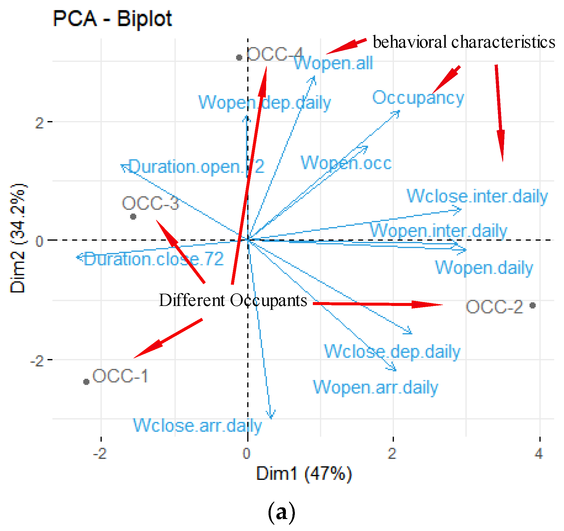
Dimensionality reduction was performed through a principal component method (PCA) to explain the 12 behavior features of each occupant with fewer variables. Figure 8a presents the distribution of four occupants and 12 variables on the two principal component axes. The “ggplot2 package” is used to visualize the 12 behavior features of different occupants. The first principal component explains 47% of the information in these 12 parameters, whereas the second principal parameter explains 34.2% of the information. It can be concluded that these two principal components explained 81.2% of the information in total, more than 80%, indicating they could explain the information of the original parameters well [45]. Hence, these two principal components could be taken for analysis.

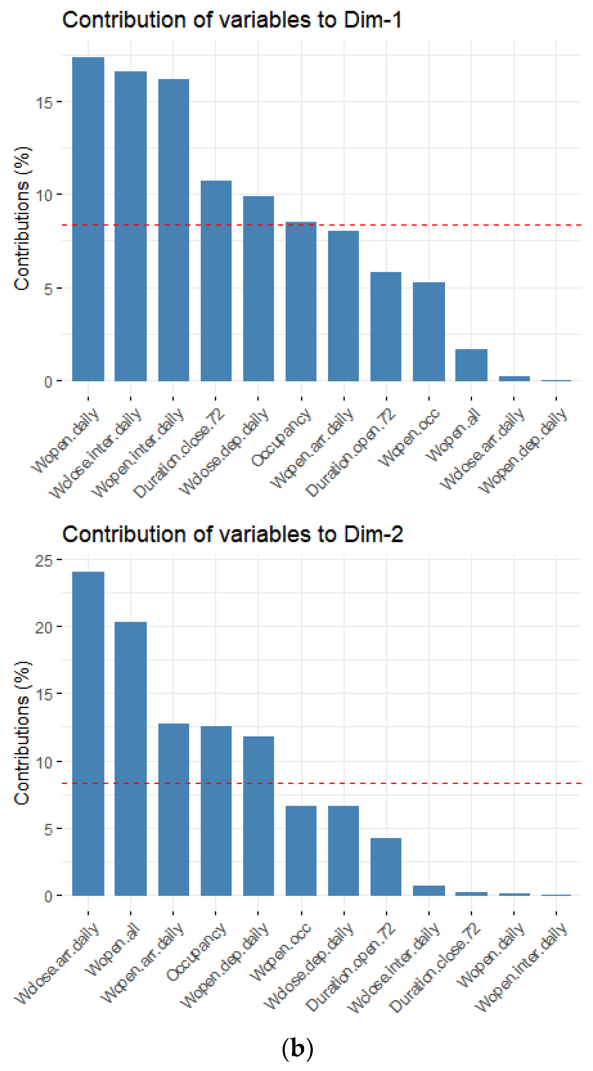
As shown in Figure 8b, respectively, variables related to dimension 1(Dim-1) and dimension 2(Dim-2) are represented, and the red dashed line represents the average contribution. It could be figured that the first principal component mainly illustrates Wopen.daily, Wclose.inter.daily, Wopen.inter.daily, Duration.close.72, Wclose.dep.daily, and Occupancy among the 12 variables, whereas the 2nd principal component mainly explains Wclose.arr.daily, Wopen.all, Wopen.arr.daily, and Occupancy, Wopen.dep.daily among these 12 varibales.

It shows that these four occupants are located at different positions on the Biplot, with significant distances (OCC-1 is on the lower left side of the figure, OCC-2 is on the right, OCC-4 is on the top, and OCC-3 is on the left), which means that their behaviors significantly varied. Wopen.daily, Wopen.inter.daily, and Wopen.arr.daily, Wclose.dep.daily are very close to OCC-2 on the map, representing that OCC-2 had a higher frequency of adjusting the window and a higher probability of opening the window when arriving and closing window when leaving office. OCC-3 is closer to Duration.open.72 and Duration.close.72. This indicates OCC-3 closed or opened windows for a longer time. OCC-1 is in the opposite direction of Occupancy and Wopen.occ, which means that the occupant spent a shorter time in the office, and the window opening duration when this occupant was in the office was low as well. OCC-4 and Wopen.dep.daily are in the same direction. Hence, it could be inferred that the occupant had a higher frequency for opening window when getting off work. Therefore, compared with the correlation coefficient graph, this biplot could reveal the behavioral similarity and diversity of different occupants directly.

3.5. Model of Regression

Figure 9A shows the indoor temperature and humidity of the four rooms and the outdoor temperature and relative humidity during the test period. As the monitoring only lasted for 40 days, it lacks the regression data and leads to difficulty in developing a model for each occupant at different times for comparison. Therefore, the data collected were aggregated and dealt with through logistics regression.

Table 4. Regression model for window use behaviors.

Behavior	Time	Regression Equation	AIC	AUC
Open	Arrival	P = 1/(1 + exp(−19.6437 + 0.3226t + 0.6137 Ti))	71.43	0.747
	Intermediate	P = 1/(1 + exp(7.38115 − 0.0578 RHo))	275.38	0.698
	Departure	None	None	None
Close	Arrival	P = 1/(1 + exp(40.2812 − 0.7071t − 1.5213Ti + 0.3786 To))	37.387	0.842
	Intermediate	P = 1/(1 + exp(−1.59732 + 0.08512t + 0.17014 Ti))	401.73	0.606
	Departure	None	None	None

Note: t is time (0–24 h), Ti and To is indoor and outdoor temperatures, RHo is outdoor relative humidity.

presents the regression model of the occupant window-opening behavior. It could be seen that the window opening/closing when arrival to the office or at the intermediate period is relative to the environmental variables and time duration, whereas there is no significant correlation between the window opening behavior at departure time and five variables. Therefore, the model of regression could not be established for departure time. Figure 9B shows the ROC curve and the corresponding AUC of window opening/closing regression model at different time periods. It could be found that the prediction accuracy of the window opening/closing models at the arrival time is relatively high, and the AUC greater than 0.7 means that the prediction accuracy of the regression model is acceptable. However, the prediction accuracy of the model at the intermediate time is relatively low as the corresponding AUC of the model is lower than 0.7. Opening the window when arriving is relevant to the time and indoor temperature. The earlier the occupant arrives at the office and the lower the indoor temperature, the more likely the occupant opens the window. Simultaneously, closing the window when arriving to the office is strongly relative to the time and indoor and outdoor temperature, among which it has the greatest correlation with time. The later the occupant arrives at the office, the more likely the occupant closes the window. Such probability would be increased by a higher indoor temperature. The window opening behavior at intermediate times is only relative to the outdoor relative humidity, whereas the window closing behavior at the same time is relative to the time and indoor temperature.

It could be seen that the windows opening behaviors in different periods are affected by different variables (the independent variables of the regression equation are different), and the significant differences exist. It should be noted that since the air conditioning operated in most cases during the monitoring period, the indoor temperature was mostly maintained at a comfortable temperature of 26–28 degrees. Therefore, the regression model fits the situation where the air conditioning is open in cooling season.

3.6. Building Energy Consumption

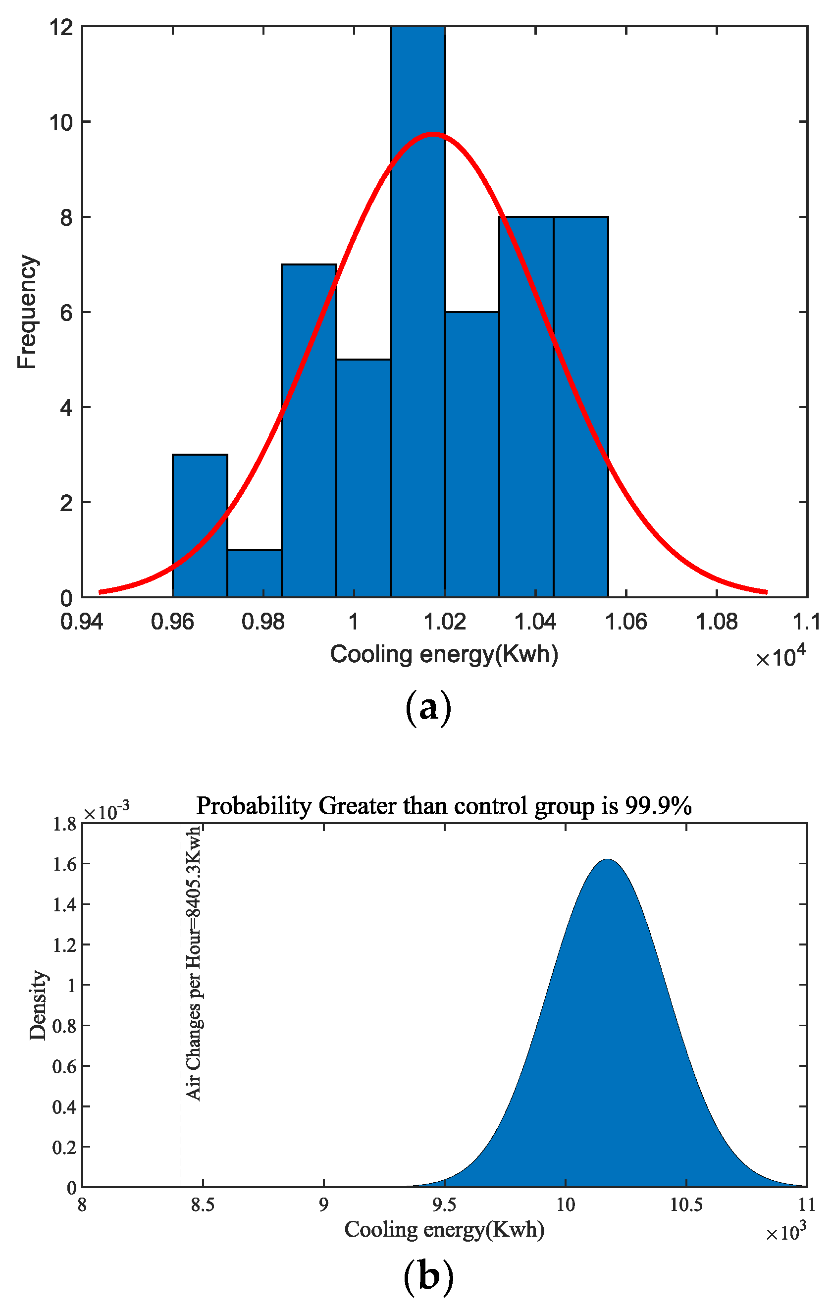
The normal distribution of cooling energy consumption of the stochastic model is shown in Figure 10a. The mean value of the data is 10,174 kwh, and the upper and lower limits are 10,243 kwh and 10,104 kwh, respectively. The red line is the Gauss Distribution. The data were found to satisfy normal distribution. The control group was ventilated according to the fixed number of air changes, and the cooling energy consumption was fixed at 8405.3 kwh. The probability density curve is shown in Figure 10b, and the cumulative distribution values are obtained by integrating. The cooling energy consumption of the stochastic model is 99.9% higher than the energy consumption generated by a fixed number of air changes, and the average energy consumption exceeds the fixed value by more than 21%.

Analyze the reason, which may be related to irrational behavior of using air conditioners and windows simultaneously for all four participants. As shown in Section 3.2, it is assumed that it is irrational if the window was opened when the outdoor air temperature was above 30 °C, as it would increase the heat gains and the consequent cooling demand.

Since green buildings have taken on energy-saving technologies, the energy-saving effect of the building envelope and the HVAC equipment is outstanding, and occupants’ behaviors (window-opening behaviors) has a greater impact on energy consumption. Therefore, the improvement of irrational behaviors contributes to reducing building energy consumption, and it is necessary to improve occupants’ behaviors. Considering that the main purpose of opening windows is ventilation and cooling, energy-saving suggestions are put forward: (1) Establish a ventilation system in the office building in time to improve air quality and (2) popularize energy-saving knowledge to minimize such behaviors.

In addition, follow-up surveys and energy consumption monitoring can be used to observe other non-energy-saving behavior in practice, to provide effective suggestions for the operation and management of other green buildings in the region.

3.7. Discussion

The case building used in this research is a three-star green building with an operation mark in Ningbo. China evaluates its buildings in accordance with the “Assessment Standard for Green Building”, and classifies them into one-star, two-star, and three-star. Three-star is the highest standard with the best energy saving effect, and only those that have been put into use for more than one year and have passed energy consumption monitoring can obtain this operation mark. It is similar to the Platinum Rated building under the LEED rating system. Compared with traditional buildings, it has better building ventilation, lighting, and energy saving strategies.

Since there are few identical buildings in Ningbo, and there are fewer occupants willing to cooperate with experiments in case buildings, there is a relatively small sample size. Previous research has found that each climate zone has its unique characteristics of window opening behavior [30]. Hence, this study can’t be extended to other cities with different environments. If there were more similar buildings in the future, we will expand the sample size for further research.

Nonetheless, some behavioral characteristics of window opening behavior have also been found by using the existing data. A statistical analysis method was conducted to reveal the similarities and differences in the window use among different occupants. With the help of the principal component analysis (PCA) of the 12 features that affected window adjustment, the correlation between the window opening behaviors and the features could be clearly illustrated. The findings of this study have certain guiding significance for promoting the energy conservation by occupants’ behaviors in green buildings in this region.

4. Conclusions

In this paper, the window opening behavior in a 3-star green building based on China’s green building evaluation standard were investigated, and four south-facing single offices were selected as a case study. The participants ranged from building energy professionals to architects. The measurement was conducted in the late summer with the use of air conditioning, and it lasted for 20–40 days. The statistical analysis was utilized to study the similarity and diversity of different occupants’ window use behaviors. The main findings are listed below:

(1)

Two types of behavior of window adjusting time were found: one is the common behavior which is opening the window in the morning and closing it in the afternoon; the other one is the opposite, whose window closing time is generally earlier than the opening time. Moreover, the occupancy duration was found to lead to significant influence on the frequency of window opening. Uncertainties were found in terms of the durations of window opening and closing for all the participants. Simultaneously, people who showed a higher frequency of window adjusting have shorter durations of window opening and closing.

(2)

This study indicates that the window adjusting times are totally different for different participants. Some are used to opening the window in the morning and closing it in the afternoon, whereas the others used to opening it when getting off work in the afternoon and closing it when getting to work in the morning. Furthermore, the participants in this study did not show the behavior of closing the window in the evening, which is different from the findings in other studies.

(3)

Some irrational window opening behavior were found in this research. For instance, when the outside air temperature was above 30 °C or even 35 °C, and the air conditioning was on, it was found that the window was still kept open for some participants. This would definitely increase the cooling energy consumption. Such a phenomenon was also found for the energy efficiency professional, although this participant is more familiar with the theories of energy saving than others. Therefore, the energy saving actions should be further enhanced.

(4)

Through correlation analysis, the total window opening duration will be longer, and the frequencies of window opening and closing will be higher with the higher occupancy rate. The higher daily window opening frequency will result in higher window opening and closing frequency at the intermediate presence. If the window is closed early in the morning, the duration of window opening will be shortened significantly. The occupant who opens window for a long time also tends to close the window for a long time and vice versa. By the principal component analysis of 12 variables influencing the window adjustment and the biplot diagram, it is shown that the correlation between the window adjustment behaviors of these four occupants and the variables (or the personality characteristics of different people’s behaviors) is visually displayed. There are significant differences among the occupants’ behaviors. If the average person model used in previous studies is used as a representative, the behavior features of the occupants will not be shown.

(5)

Through logistic regression, the regression prediction models of opening and closing at arrival time and opening and closing at intermediate time were obtained. It was found that the factors influencing window use at different times were different, and the window use behaviors at departure time was not significantly related to time or indoor and outdoor temperature. A typical office building with a fixed number of air changes per hour for the infiltration and the stochastic model of window-opening behavior was used in this paper. The cooling energy consumption of the stochastic model is 99.9% higher than the energy consumption generated by a fixed number of air changes, and the average energy consumption exceeds the fixed value by more than 21%. It shows that window-opening behavior significantly affects building cooling energy consumption.

The conclusions of this study are only applicable in cooling seasons since only the opening and closing behavior of windows during the air-conditioning period in summer was monitored. The effects of any other external environmental factors, including PM2.5, wind speed, and rainfall were not taken into consideration, leading to accuracy issues of this model. Also, only four single offices and one building energy efficiency professional were involved. This will result in deviations when comparing the similarities and differences in behavior between building energy efficiency professionals and ordinary people. Therefore, future research will focus on the above-mentioned shortcomings. More detailed studies will be carried out, which will cover more samples. The monitoring time will be increased, and the window opening behavior of ordinary buildings in the region will be compared and analyzed to obtain more accurate predictions.