Estimating the Drivers of the Cost of Saved Electricity in Utility Customer-Funded Energy Efficiency Programs

Abstract

Energy efficiency programs funded by utility customers provide an electricity resource in most U.S. states, but their scale and cost of saving electricity varies significantly by state. In this paper, we explore the drivers of the cost of saved electricity in these programs with an econometric model and nearly a decade of data reported by efficiency program administrators. We found strong evidence for economies of scale and weak evidence for diseconomies of scale, which suggests that states with low levels of efficiency savings relative to retail sales can increase the size of their efficiency programs without large increases to the cost of saved electricity. We discuss examples of energy efficiency forecasting and potential modeling in light our econometric analysis and identify methodological improvements relevant to utilities and grid operators. This paper provides insights into the economics of customer-funded efficiency programs that will support regulators, utilities, and policymakers to utilize energy efficiency as a resource.

1. Introduction

Utility customer-funded electricity efficiency programs provide a low-cost electricity resource in 42 states, with investments in 2018 totaling more than USD 5.8 billion and savings exceeding 34 terawatt hours (TWh) [1]. Understanding the cost drivers of customer-funded energy efficiency portfolios can help facilitate regulatory oversight of these programs, help utilities better utilize energy efficiency as a resource, and inform building energy decarbonization policies.

Insight into differences between the cost of saved electricity across states and utilities can help regulators benchmark performance and set appropriate spending levels for utilities in their jurisdictions. Similarly, utilities can use this information to develop least-cost investments in efficiency. In particular, regulators and utilities can benefit from understanding how the cost of saved electricity relates to the scale of the efficiency resource portfolios. For example, increased savings levels may introduce operational efficiencies that reduce the cost of saved electricity. However, historical investments in certain efficiency measures may reduce the availability of low-cost efficiency savings and could counteract this effect. Quantification of these economies and diseconomies of scale, therefore, would be valuable to regulators and utilities estimating the remaining efficiency potential and forecasting spending.

Policymakers can leverage an understanding of drivers of the cost of saved electricity to inform long-term decarbonization strategies. First, insight into the cost of saved electricity can help grid operators assess the role of energy efficiency as a demand-side resource alongside traditional supply-side generation resources. For example, the New England Independent System Operator (ISO New England) uses the cost of saved electricity reported by efficiency program administrators (the organizations that implement energy efficiency programs funded by electricity and gas customers) as part of its efficiency forecasting methodology [2]. Second, when the cost of saved electricity is coupled with information on the timing of efficiency savings, policymakers can better evaluate efficiency as a capacity resource that can reduce peak demand. For example, energy efficiency measures can provide significant value to the grid during peak demand periods but its role as a peak resource depends on whether it is cost competitive with generation and other distributed energy resources [3].

The economics of customer-funded energy efficiency programs can also inform policies that promote building electrification, demand flexibility, and reduce risks from extreme heat. Electrification efforts may exhibit economies of scale similar to those of efficiency programs, in particular for residential buildings, given that they incentivize similar measures (e.g., heat pumps) and employ similar implementation strategies (e.g., upstream incentives) [4]. Similarly, programs that seek to mitigate the impacts of extreme heat may draw on measures generally associated with energy efficiency, such as building envelope improvements [5]. Recent state-level efforts at managing extreme heat risk have also identified existing efficiency programs as implementation mechanisms [6]. Finally, recent research into the technical potential for demand flexibility in U.S. buildings finds synergies in the co-deployment of efficiency and flexibility measures [7]. Estimates of the economic potential for demand flexibility would, therefore, likely benefit from an understanding of the economics of large-scale efficiency program investments.

Several studies have documented the cost of saved electricity from energy efficiency programs. For example, research has characterized how the cost of saved electricity in programs administered by American investor-owned utilities varies geographically, temporally, and by market sector [8,9]. Similar work has described the cost of saved electricity for publicly owned American utilities [10]. Internationally, researchers have examined the cost of saved electricity for both state and utility-administered energy efficiency programs in Korea [11,12].

Additionally, the literature also includes studies that employ econometric methods to explain variation in the observed cost of saved electricity. Arimura et al., 2012 estimates the effect of past and current energy efficiency program spending based on changes in electricity demand using a parametric function and non-linear model as well as utility-fixed effects [13]. Arimura et al., 2012 then predicts the lifetime savings of efficiency investments made in the study period 1992–2006 and calculates an average cost of saved electricity under a range of discount rates [13].

Hoffman et al., 2017 considers both a linear and quadratic relationship between the program administrator levelized cost of saved electricity and program year using program administrator fixed effects for programs implemented between 2009 and 2013 [14]. Overall, the authors find mixed results on the significance of program year on the cost of saved electricity. The study does not find statistically significant results at a 95% confidence interval when the model only includes the linear program year term. With the addition of a quadratic program year variable, the quadratic term is significant at a 95% confidence interval and the linear term is just barely not significant (p-value of 0.059). The negative linear term and positive quadratic term suggests that the cost of saved electricity declines before reaching a minimum and increasing. Hoffman et al. (2017) also considers models of the same structure on the cost of saved electricity for different types of programs (e.g., residential lighting) [14]. Using data reported in Energy Information Administration (EIA) Form 861 for the period 2010–2019, Knight et al., 2022 explores economies of scale in energy efficiency programs by regressing the program administrator levelized cost of saved electricity on each program administrator’s first year savings as a percent of its retail sales in a given year [15]. The authors find a downward linear trend, suggesting that energy efficiency programs have economies of scale. Their model, however, only explains 12% of the observed variation in the levelized costs and does not include any fixed effects.

This study continues a line of research that uses econometric techniques to estimate the costs of saved electricity in customer-funded energy efficiency programs. We build on these analytic efforts by considering economies of scale with annual savings as a percent of sales among a broader set of covariates, including construction labor costs and both time and program administrator fixed effects. As

Table 1. Comparison of econometric models of the cost of saved electricity.

				Covariates
Study	Data Source	Period	Level of Analysis	PA Fixed Effects	Year Fixed Effects	Labor Costs	Annual Savings as % of Sales	Cumulative Savings as % of Sales
Arimura et al., 2012 [13]	EIA Form 861	1992–2006	Portfolio	Yes	Yes	No	No	No
Hoffman et al., 2017 [14]	Utility regulator reports	2009–2013	Portfolio, lighting programs	Yes	Yes	No	No	No
Knight et al., 2022 [15]	EIA Form 861	2010–2019	Portfolio	No	No	No	Yes	No

PA stands for program administrator.

summarizes, no model in the literature includes all of these covariates. We address a gap in the literature of econometric analyses of the cost of saved electricity by introducing a variable for historical efficiency achievement–cumulative efficiency savings as a percent of sales. We include this variable to explore potential diseconomies of scale that result from the increasing costs of achieving remaining energy efficiency potential. Past research has conceptualized energy investments as a supply curve in which different technologies and approaches deliver different levels of savings at different costs [16]. If historical energy efficiency efforts are focused on the less costly sections of the efficiency supply curve, the remaining potential would be weighted towards the more expensive end of the supply curve. In this case, we would expect increases in cumulative savings as a percent of sales to increase the cost of saved electricity. We incorporate this variable into our regression model and explore how it varies across states and in between customer segments. We employ a weighted least squares model to account for differences in the size of the efficiency programs.

2. Materials and Methods

2.1. Energy Efficiency Program Data

We constructed a dataset of program costs, energy savings, and savings lifetimes on gas and electric energy efficiency programs administered by investor-owned utilities, publicly-owned utilities, government agencies, and third parties. We primarily source these data from annual regulatory reports that utilities file with state energy regulators. In some cases, we acquired program data directly from utilities and from databases and dashboards maintained by regulatory agencies.

The format of the reported program data was typically in tables embedded in PDFs, which we transcribed into a collection template. We assigned each program to a standard program type developed by the Lawrence Berkeley National Laboratory [17]. To prepare the data for analysis we implemented a two-staged review process. First, we manually reviewed the transcription of the reported data. Second, we identified potential data-entry errors by flagging any program with unexpectedly low or high first year costs of saved electricity (below USD 0.01/kWh or above USD 50/kWh). We then manually reviewed the data for any flagged program and compared it with its source. Therefore, we did not reject outliers simply because of high or low costs of saved electricity; we based our analysis on what utilities reported and conducted data cleaning procedures to assure that we accurately represented the reported data. We drew on more than 5500 program-years of these data to build a panel dataset of 32 program administrators in 14 states that operated electric efficiency programs between 2010 and 2018. In 2018, these program administrators accounted for 55% of savings reported by investor-owned utilities to the EIA in the same year (EIA 2019).

In our analysis, we used ex ante estimates of gross savings for each program as reported by program administrators to state regulators in annual filings. They did not include free-rider or spillover effects nor did they account for evaluation, measurement, and verification (EM&V) studies that occurred in the reporting year. For costs, we included all of the costs that an energy efficiency program administrator would incur, including costs for administration, marketing, evaluation, and customer incentives. We did not include the costs participants incurred as part of participation nor the cost of any shareholder incentive that may have resulted from program achievement. 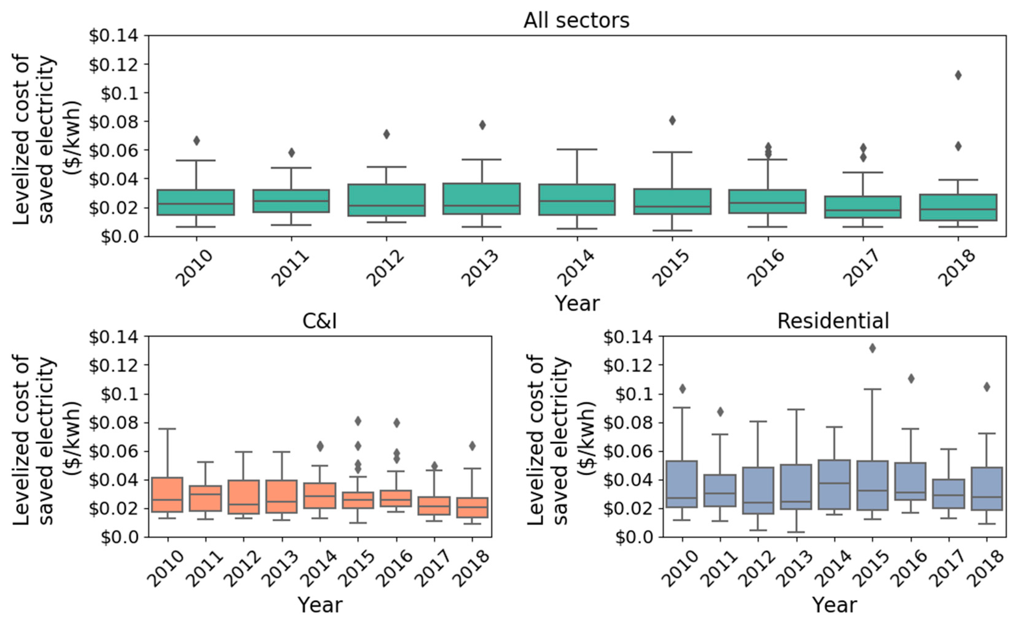For each program administrator and year, we calculated the levelized cost of saved electricity, which amortizes the cost of an efficiency program over the lifetime of the program’s savings [18]. We define three market sectors: commercial and industrial (C&I) and residential, which also include programmatic offerings for low-income customers, and cross-cutting, which includes programs that serve multiple customer classes.

In

Table 2. Share of aggregate gross electricity savings and program administrator spending by state.

State	Share of Aggregate Gross Electricity Savings	Share of Aggregate Program Administrator Costs	Program Count
Arizona (AZ)	4.0%	2.4%	131
California (CA)	24.0%	26.0%	1553
Colorado (CO)	3.8%	3.1%	380
Massachusetts (MA)	12.1%	19.7%	696
Maryland (MD)	5.2%	6.2%	400
Michigan (MI)	9.9%	7.4%	340
Minnesota (MN)	4.9%	3.5%	554
North Carolina (NC)	4.5%	2.9%	128
New Jersey (NJ)	3.9%	4.8%	117
New York (NY)	6.4%	6.4%	247
Oregon (OR)	4.7%	5.4%	48
Pennsylvania (PA)	13.7%	9.5%	653
Texas (TX)	0.6%	0.6%	217
Utah (UT)	2.4%	2.1%	86

and

Table 3. Share of aggregate gross electricity savings and program administrator spending by market sector.

Market Sector	Share of Aggregate Gross Electricity Savings	Share of Aggregate Program Administrator Costs	Program Count
Residential	40.9%	40.2%	2156
C&I	49.4%	53.0%	2402
Cross Cutting	9.7%	6.9%	992

, we show the composition of the panel dataset in terms of the states and market sectors. Across the nine years of program performance in our dataset, three states: California, Massachusetts and Pennsylvania account for 55% of spending and nearly 50% of savings. Combined, their 2900 records of program are 52% of all of the programs in the dataset. C&I programs account for about half of savings and spending, with 40% resulting from residential programs and the remainder from cross-cutting programs. The five most common program types in our dataset, in terms of overall gross electricity savings, were residential lighting, codes and standards, general prescriptive C&I, custom C&I, and residential behavioral programs. These program categorizations are consistent with Hoffman et al., 2013 [17]. Together, these programs account for 48% of the reported electricity savings in our dataset.

2.2. Annual and Cumulative Savings as a Percent of Sales

We measured program scale relative to a utility’s sales base using two metrics: annual savings as a percent of annual retail sales and cumulative savings as a percent of annual retail sales. We calculated annual savings as a percent of sales by dividing annual electric efficiency savings by annual retail sales as reported in EIA 861. Where a program administrator’s impacts were broader than one utility jurisdiction, we aggregated the savings and sales from the applicable utilities. To characterize the composition of each program administrator’s sales base, we calculated the share of retail sales only from residential and C&I customers in each year. We also measured program scale by customer class by calculating annual residential and C&I savings as a percent of retail sales for each program administrator.

We used cumulative savings as a percent of sales to measure the scale of savings from past investments in energy efficiency that have not reached the end of their useful life. We used reported savings lifetimes to estimate when program savings expire. Program administrators reported lifetimes for half of the programs in our dataset. For the remaining programs, we estimated lifetimes based on the lifetimes reported for the same program type. For a given year, we aggregated the savings from prior years that have not expired, regardless of when they began, and divided them by retail sales in that year. For example, a program administrator’s cumulative savings in 2018 would reflect all of the savings from program investments made between 2010 and to 2017 that are still active. If a program administrator reported in 2012 that savings from an efficiency program in that year would last 7 years, we would include those savings in the cumulative savings for each year 2013–2018. Cumulative savings as a percent of sales, therefore, can exceed annual savings as a percent of sales, particularly in later years. We did not include savings from before 2010 in this calculation. While some savings from years prior to 2010 likely continue through our analysis period, we lack the data to quantify their contribution. Program administrator fixed effects in the regression model address this issue as cumulative saving pre-2010 are time invariant characteristics of administrators.

2.3. Regression Analysis

2.3.1. Base Model

We quantified drivers of the cost of saved electricity through a regression analysis and built on past econometric efforts by accounting for the impact of cumulative energy efficiency savings. Given that our sample includes both small and large investor-owned utilities (the largest annual electricity sales for a single utility is 26 times the smallest annual sales in our dataset), we employed a weighted least squares model with annual retail sales as weights. We specify the regression model in Equation (1). The subscripts on the covariates indicate the dimensions in which the covariates may vary: time (t) and program administrator (PA). The main covariates of interest are annual savings as a percent of sales (S) and cumulative savings as a percent of sales (C). Furthermore, we used two types of fixed effects in our model. Calendar year fixed effects (μ_t) account for factors that vary in time but are common to each administrator, such as macro-economic conditions or the impact of federal appliance efficiency standards. Program administrator fixed effects (η_PA) account for factors that are static in time but vary with each administrator such as differences in program administration, service territory, or regulatory environment. We also addressed how state-level differences and changes in labor costs may affect the cost of saved electricity with an annual Employment Cost Index (γ_t) for construction workers published by the Bureau of Labor Statistics [19]. We also included the savings-weighted lifetime (λ_PA,t) of each program administrators’ efficiency portfolio in each year of the study period as it is an input into the formula for the levelized cost of saved electricity [18]. Finally, we included an intercept (α) to capture baseline costs of energy efficiency program administration.

Cost of saved electricity = α + μ_t + η_PA + γ_t + S_t,PA + C_t,PA + λ_PA,t

(1)

2.3.2. Additional Covariates

We explored the impact of several covariates in addition to those in the base model. First, we considered whether differences in the customer composition of utility jurisdiction affects the cost of saving electricity. Given that C&I programs are generally less costly than residential programs, a larger C&I customer base could provide a reliable source of low-cost efficiency savings [20]. We tested this hypothesis by including the share of total sales from C&I customers as a covariate. To account for differences in the cost of saved electricity between customer segments, we also included the share of each program administrator’s annual savings from C&I, residential, and low-income programs.

2.3.3. Alternative Dependent Variable

Next, we tested sector-specific versions of our dependent variable (e.g., the levelized cost of electricity for C&I programs only) and adjusted program scale covariates accordingly. A regression of the levelized cost of electricity only for C&I programs, then, would be on annual and cumulative C&I savings as a percent of sales. Since EIA 861 does not separate residential sales into low income and non-low-income as many program administrators do for their programs, we included low-income programs in the residential levelized cost of saved electricity.

2.3.4. Alternative Sample

As robustness check against compositional effects, we apply the base model to a sample that covers a shorter time period 2011–2018 and but includes six more program administrators (38 total) than our base sample and a non-panel dataset that covers 2010–2018 and 117 program administrators.

3. Results

3.1. Cost of Saved Energy over Time

Figure 1 shows how the cost of saved electricity changes between 2010 and 2018 for all sectors combined and for each sector (C&I and residential) separately. Each data point represents the cost of saved electricity for a program administrator in a given year, with the boxes displaying the interquartile range in each year. The bottom of the box is the 25th percentile, the horizontal bar is the 50th percentile, and top of the box is the 75th percentile. The whiskers extend to the last data points that are within a distance 1.5 times the interquartile range above the top and below the bottom of the box. The diamonds represent any values beyond the whiskers. Overall, the median cost of saved electricity declines by about USD 0.005/kWh from USD 0.026/kWh to USD 0.021/kWh after increasing in the middle of the time period. C&I programs exhibit a similar decline, beginning at USD 0.022/kWh and ending at USD 0.018/kWh. In contrast, we found a slight increase (USD 0.001/kWh) in the median levelized cost of electricity for residential programs between 2010 and 2018. Residential programs also display more variation than C&I programs, largely due to their inclusion of low-income programs in the former, which are typically more expensive than market-rate residential efficiency programs [20].

3.2. Scale of Programs

In Figure 2, we present the program administrator’s levelized cost of saved electricity against annual savings as a percent of sales in each year. Each data point represents a program administrator’s cost of saved electricity for a single program year between 2010 and 2018 against its retail sales in that year. Program administrators have a wide range of savings levels and costs of saved electricity that reflect efficiency portfolios at different stages of development. Within our sample, regional differences emerge. The program administrators with the lowest and highest levels of savings are largely in the South and Northeast, respectively. In both regions, however, there is a wide range of costs of saved electricity. Overall, Figure 2 does not reveal a simple relationship between program scale and the cost of saved electricity.

Figure 3 shows cumulative savings as a percent of sales by state and customer segment in 2018. Differences in annual savings between administrators compound over time, resulting in a wide spread of cumulative efficiency savings by the end of our study period. For example, program administrators in Massachusetts have the highest levels of cumulative savings across all customer segments, equivalent to nearly 20% of retail sales in 2018. In contrast, program administrators in Texas have cumulative savings levels less than two percent of retail sales. In most states in our sample for 2018, cumulative residential savings as a percent of residential sales are higher than cumulative C&I savings as a percent of C&I sales.

These differences accord with the overall relationship that we observed between sales and savings for residential and C&I programs in our dataset. In 2018, C&I customers account for 65% of sales and 46% of first year savings, whereas residential customers account for 35% of sales and 39% of savings. This trend suggests that significant commercial energy efficiency opportunities may remain for C&I customers in the states in our sample.

3.3. Regression Results

We found that energy efficiency programs in our base sample display both economies and diseconomies of scale, are sensitive to construction labor costs, and exhibit both year and program administrator fixed effects. Together, these factors explain 64% of the observed variation in the levelized cost of saved electricity in our dataset. We summarize these results in

Table 4. Program administrator and program year fixed-effects model with weighted least squares.

	Levelized Cost of Saved Electricity
	All Sectors
Annual savings as percent of sales	−0.591 ***
	(0.152)
Cumulative savings as percent of sales	0.137 **
	(0.061)
Savings lifetime	−0.001 ***
	(0.000)
Employment Cost Index	0.025 ***
	(0.006)
Intercept	0.029 ***
	(0.003)
Observations	288
R2	0.637
Adjusted R2	0.575
Residual Std. Error	40.285 (df = 245)
F Statistic	46.330 *** (df = 42; 245)

Note:** p < 0.05; *** p < 0.01.

.

As the scale of the program (measured as the annual savings as percent of sales) increases, we found that the levelized cost of saved electricity decreases. For a 1% increase in annual savings as a percent of sales, all else being equal, our model estimates a USD 0.006/kWh decrease in the levelized cost of saved electricity. In contrast, the cost of saved electricity increases by about USD 0.14/kWh for a 1% increase in cumulative savings as a percent of sales. The positive return to scale from an increase in annual savings levels, importantly, is more than four times the negative return to scale of an equivalent increase in the cumulative savings level. Since cumulative savings as a percent of sales can increase while annual savings as a percent of sales remains constant, these results suggest that the diseconomies of scale could offset the economies of scale. However, while annual savings as percent of sales is a statistically significant predictor of the levelized cost of saved electricity in the 2011–2018 sample, cumulative savings as a percent of sales is not (see Appendix A for results of alternative model specifications). Additionally, we found that annual savings as a percent of sales is a significant predictor for the residential and C&I levelized cost of saved electricity (see Appendix A for regression results). Cumulative savings as a percent of sales is nearly a significant predictor for the C&I and not for the residential levelized cost of saved electricity at a 95% confidence interval. Overall, our findings provide strong evidence that energy efficiency programs exhibit economies of scale and weak evidence for diseconomies of scale during this time period.

Next, we found that the 17% growth in the construction Employment Cost Index between 2010 and 2018 increases the levelized cost of saved electricity by about USD 0.005/kWh. For the C&I levelized cost of saved electricity, the index is also a statistically significant predictor and has a somewhat larger effect on costs over the study period (USD 0.008/kWh). We did not find a statistically significant impact of the index for the residential levelized cost of saved electricity. This result may reflect the differences in the labor markets of commercial and residential energy efficiency programs. Commercial programs may draw on a workforce more similar to construction jobs tracked by the Employment Cost Index than do the residential programs.

We also found statistically significant program administrator fixed effects in our base model and across all alternative specifications and samples. Each effect is relative to a base program administrator, National Grid Massachusetts, which we selected because it had the highest cost of saved electricity among program administrators in our sample. To explore whether program administrator effects were only different from just National Grid Massachusetts or more generally from each other, we performed pairwise t tests of each effect’s regression coefficient against each other’s effect regression coefficient. For each program administrator, we found a significant difference at a 99% confidence interval between its effect and those of the majority of the other program administrator effects. These tests indicate that the program administrator effects are not just different from those of our base program administrator, but from each other more broadly. Furthermore, they underscore the importance of the program administrator effects in explaining variation in the cost of saved electricity. We summarize the program administrator fixed effects results in Appendix A.

The year fixed effects show a decline in the cost of saved electricity across all of the program administrators in our base model, all else equal. This trend of declining fixed costs may reflect the maturation of the energy efficiency industry in our sample through the availability of lower cost vendors and equipment. Full results for the year fixed effects are in Appendix A. We found that these results also hold for the 2011–2018 sample, but not for the non-panel dataset, which may reflect the non-panel dataset’s imbalanced coverage of the time period.

Unsurprisingly, we found that the savings lifetime has a small but significant effect on the levelized cost of saved electricity. For a one year increase in savings lifetime, the levelized cost of saved electricity declines by USD 0.001/kWh. We would expect this result by construction since levelized cost is a function of spending, savings, and lifetime.

4. Discussion

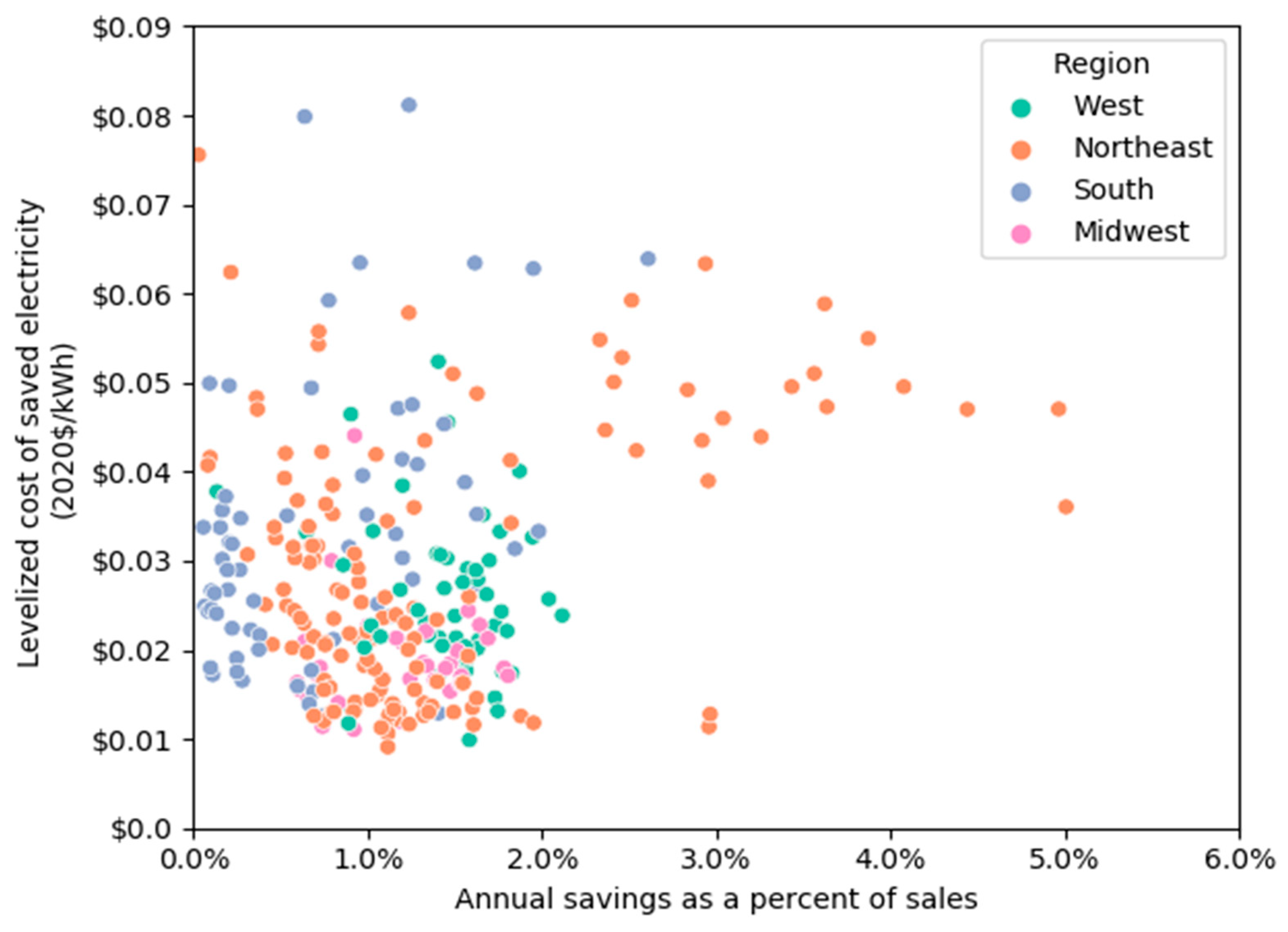
Our regression analysis generally aligns with the results of similar work and provides new evidence for other drivers of the cost of saved electricity. First, we found a strong economies of scale: as annual savings as a percent of sales increases, the cost of saved electricity decreases at the portfolio level and for residential and C&I programs separately, all else being equal. In contrast, Knight et al., 2021 concludes that annual savings as a percent of sales and the cost of saved electricity only displays a weak relationship [15]. Additionally, we found some evidence for diseconomies of scale in customer-funded efficiency programs through our estimate of cumulative efficiency savings, though the result was not robust to our alternative model specifications and warrants additional research. Together with employment costs and program administrator and year fixed effects, these measures of program scale explain the majority of the observed variation in the cost of saved electricity (R² = 0.637), much higher than the 12% explained by the model in Knight et al. [15]. Future research could build on this work by exploring the impact of various policy variables on the cost of saved electricity. For example, higher avoided costs would allow more costly programs to pass cost-effectiveness tests, thereby putting upward pressure on the cost of saved electricity. Conversely, higher discount rates in screening tests could select for less costly programs.

Our regression results demonstrate the importance of programs scale-as measured by annual savings as a percent of sales-on the cost of saved electricity. Energy efficiency forecasting and potential study methodologies, however, do not always reflect this relationship. For example, in its energy efficiency forecasts, ISO New England uses a deemed cost escalation factor that reflects measure penetration and technology costs. The escalation factor is graduated, beginning at 0% in the first year of the forecast and increasing by 1.25% each year thereafter [2,21]. These factors linearly increase the cost of saved electricity in each year of the forecast, regardless of any economies of scale. Since ISO New England forecasts savings as a function of budgets and the cost of saved electricity, these escalation factors put downward pressure on savings forecasts. The results of our regression analysis, however, suggest a more nuanced approach to estimating the cost of saved electricity is warranted. In the context of ISO New England’s forecasts, annual and cumulative savings as a percent of sales, program administrator effects, and labor costs may all contribute to more accurate cost projections.

Simplistic assumptions about the cost of saved electricity also affect energy efficiency potential studies. As part of its 2020 integrated resource plan, Duke Energy commissioned a study of its energy efficiency savings potential. The study included an ‘Enhanced Scenario’ in which incentives double but energy savings only increase by 6.3% on average relative to a base case scenario [22]. The economies of scale that we found imply that such significant increases in incentive levels are not necessary for higher levels of savings. Similarly, a 2020 efficiency potential study for Evergy assumes that the first year cost of saved electricity declines as savings levels increase for most commercial programs but not for residential programs [23]. Our results, however, suggest that economies of scale apply to both residential and commercial programs. In general, models of energy efficiency savings potential should account for economies of scale. However, we are less confident in applying the diseconomies of scale from our regressions to efficiency potential models since this result was weaker than that for the economies of scale.

These examples of how energy efficiency forecasts and potential studies are illustrative but not necessarily representative. Still, they illustrate how empirical estimates of the cost of saved electricity are relevant for utilities, regulators, and policymakers. Additional research into energy efficiency forecasting and potential study methodologies would help characterize industry trends in projecting the cost of saved electricity. Programmatic efforts for demand flexibility, building electrification, and extreme heat mitigation may also find these results relevant given potential similarities in implementation to efficiency programs.

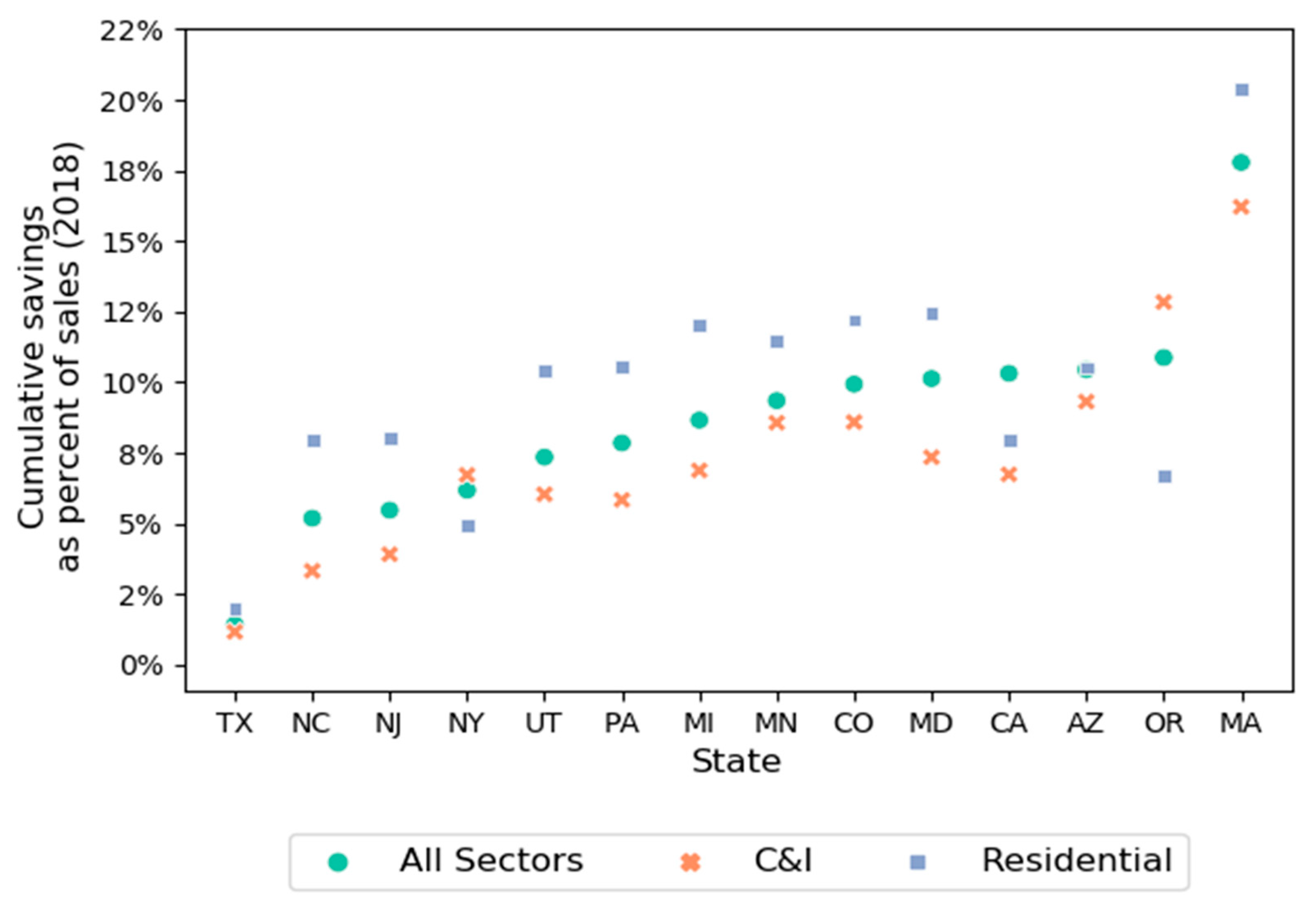
The differences we observed in state-level cumulative savings may reflect the existence of an efficiency achievement gap. Importantly, energy efficiency savings do occur outside of customer-funded programs, including through building codes, appliance and equipment standards, and private investment. Higher rates of investments in energy service companies’ (ESCO) projects may compensate for lower customer-funded savings levels. For example, New York is in the bottom half of cumulative savings achievement in our sample but has relatively high rates of ESCO investment [24]. In contrast, Texas has the lowest cumulative savings in our sample and only moderate levels of ESCO investment, which suggests that the state may have significant remaining efficiency potential [24]. The economies of scale in our regression model suggest that Texas or a similar state with lower levels of overall energy efficiency achievements can increase efficiency savings goals without significant increases and possible with decreases in the cost of saved electricity.

Our analysis produces quantitative results that are specific to energy efficiency programs administered by investor-owned utilities in the U.S. However, some qualitative results are relevant to policymakers in other countries that have utility- or state-led energy efficiency programs [11,12,25]. In particular, our evidence for economies of scale may be informative to policy conversations on levels of investment and be relevant to jurisdictions developing energy efficiency forecasts or potential estimates. While our dataset includes program administrators that account for more than half of energy efficiency savings reported by investor-owned utilities to the IEA in 2018, it does not include administrators from every state. Additionally, our dataset covers the years 2010–2018 and does not include data from efficiency programs operating in the wake of the COVID-19 pandemic, during which lockdowns shifted electricity usage towards residential buildings [26] and the energy efficiency sector experienced significant job losses [27]. Analysis of an expanded panel dataset that includes data for the years 2019–2022 would shed light on whether the effects we observed for 2010–2018 have continued.

5. Conclusions

In this study, we leveraged nearly a decade of data on utility customer-funded energy efficiency programs to examine drivers of the cost of saved electricity through a regression model. We found strong evidence for economies of scale and weaker evidence for diseconomies of scale in program energy savings levels. These results are relevant to system operators forecasting efficiency, utilities estimating efficiency potential, and policymakers considering investments in energy efficiency or exploring strategies for building electrification, demand flexibility, and extreme heat mitigation. Furthermore, we documented large differences in state-level cumulative energy efficiency savings that may suggest an efficiency achievement gap. Our regression analysis suggests that states’ savings can overcome this gap and increase energy efficiency savings levels without significantly increasing the cost of saved electricity. Future research can build on this work by including efficiency program data from more states and from more recent years, including those after the COVID-19 pandemic. Such research could test whether the effects we observed for 2010–2018 have continued and could explore the significance of cumulative savings as a percent of sales on the cost of saved electricity.