Article

The Relationship between Energy Consumption and Economic Growth in the Baltic Countries’ Agriculture: A Non-Linear Framework

1
Department of Applied Economics, Finance and Accounting, Faculty of Bioeconomy Development, Agriculture Academy, Vytautas Magnus University, 53361 Kaunas, Lithuania
2
Institute of Economics and Regional Development, Latvia University of Life Sciences and Technologies, 3001 Jelgava, Latvia
*
Author to whom correspondence should be addressed.
Energies 2023, 16(5), 2114; https://doi.org/10.3390/en16052114
Submission received: 4 February 2023 / Revised: 18 February 2023 / Accepted: 20 February 2023 / Published: 22 February 2023
(This article belongs to the Special Issue Energy Consumption in the EU Countries II)

Abstract

:
The development of a country’s economy is directly related to the use of energy in that country’s economic sectors. Therefore, the energy–environmental Kuznets curve (EEKC) is often used when analysing a country’s potential and challenges in sustainable development, green economy, and green growth. This hypothesis tests whether there is an inverse “U”-shaped relationship between energy use and economic growth and is especially important when analysing developing countries to assess if, at a certain point, energy use begins to drop, resulting in fewer greenhouse gas emissions, environmental degradation, and the consumption of fossil-based fuels. This study aims to examine the relationship between energy consumption and economic growth in the Baltic States from 1995 to 2019, with a focus on the agriculture sector. The study uses the non-linear autoregressive distributed lag (NARDL) model for individual and panel time series. Total energy use, as well as electricity use, is included in the study, whereas gross value added is employed as a measure of economic growth. Research data analysis reveals that energy use in all three Baltic countries stabilises as gross value added increases. However, there is insufficient evidence to show that after a certain point, energy use begins to drop; thus, the hypothesis for the inverse “U”-shaped energy–environmental Kuznets curve (EEKC) is rejected. Research results have important practical implications regarding countries’ policies toward energy, including the use of electricity and sustainable development.

1. Introduction

In recent decades, climate change has become a global phenomenon, and its effects are becoming more and more evident. It threatens the environment, biodiversity, economic activity, and sustainable development. In addition, economic development has a significant impact on climate change and sustainable development [1]. It is recognised that sustainable environmental quality must be an essential part of sustainable economic development [2]. Scientists often associate better environmental quality with the reduction of greenhouse gas emissions, especially carbon dioxide (CO2) emissions [3,4,5,6]. However, the development of economic activity is often associated with environmental degradation [7], and thus with negative effects on the climate. The world’s largest amount of GHG emissions is produced by energy production: 87% of total GHG (2020) [8]. This problem must be solved primarily by improving energy use efficiency [9,10], developing and implementing clean production technologies, and increasing natural GHG absorbers [9]. It is characteristic of the economy as a whole and its individual sectors, including agriculture.
Energy resources are essential both for households to meet their personal needs and economic activities in the production of goods and services. Energy is used in many sectors: industry (production of iron, steel, fertilisers, pharmaceuticals, production of food products and tobacco products, non-ferrous metals, paper, textiles, machinery and equipment, extraction of oil and gas and so on), transport (burning gasoline and diesel for all types of road transport, aviation, shipping, the railway sector, fuel and raw material transportation by pipelines, among others), residential and commercial buildings, agriculture, forestry, fishing, and the like. The production of heat and electricity emits the most GHG in the world [11]. In 2019, emissions from this sector amounted to 15.83 billion metric tonnes [12]. It is predicted that world energy-related CO2 emissions will increase to 43.2 billion metric tonnes in 2040 [13]. The main driver of these pollutants is the increasing demand for energy, mainly obtained by burning fossil fuels [14,15].
Economic expansion and energy consumption have an interactive and complementary relationship [4]. In order to reduce the amount of GHG emissions and at the same time the negative impact on the climate, energy efficiency is essential. Energy efficiency is usually evaluated in terms of energy intensity [16,17], which shows the energy consumption to perform a specific process or produce a product in a country. It is a way to measure the relationship between energy consumption and economic growth [18]. The energy efficiency policy aims to produce more with less energy.
Although energy is the driver of the economy, it can lead to the deterioration of the quality of the environment [19]. Therefore, the economy must develop with less energy consumption. In other words, it is important to decouple economic growth from energy consumption when increasing energy efficiency. As energy efficiency increases, more benefits are obtained: GHG emissions, air, water, and soil pollution would be reduced; fewer resources would be used to extract, transform, transport, and use energy; as well as additional benefits related to the state of ecosystems [20].
As part of the European Green Deal, the EU has increased its ambitions in the field of increasing energy efficiency and aims to reduce primary and final energy consumption by at least 32.5% by 2030 at the EU level (compared with the energy consumption forecasts for 2030) [10]. Eurostat data also show that the decoupling of economic growth and energy consumption is increasing due to the EU’s comprehensive energy efficiency policy [20,21]. Economic growth is one of the main goals of every country. It relates to energy use, and the latter to environmental impact. The interaction between energy consumption, economic growth, and environmental quality is rather controversial. Policy makers, therefore, face a significant challenge in balancing the goals of economic growth, energy use, and environmental impact. If energy is used inefficiently, the negative consequences for the economy are huge [22]. Therefore, countries are looking for ways to achieve sustainable development while reducing fossil fuel energy consumption and achieving economic growth [23].
The energy–environmental Kuznets curve (EEKC) can be used to determine the relationship between energy use and economic growth. The theory explains that an increase in energy consumption is accompanied by economic growth in the early stages of economic development, and after a tipping point in the later stages of economic development, energy consumption decreases as energy efficiency increases [24]. EEKC hypothesises that there are inverted U-shaped or N-shaped relationships between energy use and economic growth and development [25].
Conducted studies show that scientists and researchers often examine the relationship between environmental pollution (measured by GHG emissions) and economic growth and test the environmental Kuznets curve (EKC) hypothesis [26,27,28,29,30]. Since, as already mentioned earlier, the majority of GHG emissions are related to energy consumption, the research examines the relationship between energy consumption and economic growth and its directionality, and recent research expands and tests the energy–environmental Kuznets curve (EEKC) hypothesis.
It must be stated that EKC and EEKC are characterised by certain limitations and are criticised for both methodological and theoretical reasons: (i) EKC is based on the assumption that economic development directly leads to environmental degradation, different sources of pollution are used to assess it, there is no apparent interaction between pollution reduction demand and supply of instruments [31]; (ii) the unclear interaction between economic development and pollution levels taking into account the country’s social system and national context [32]; (iii) with increasing technological progress and energy efficiency, energy costs may not only decrease, but may even increase [33,34]. Cheaper energy costs due to an increase in its use efficiency can encourage its consumption, which could increase the negative impact on the environment and climate change; this is referred to as Jevons’ paradox [35]. This problem is highly relevant in agriculture since increased energy efficiency would result in increased agricultural production volumes and thus accelerate processes related to soil erosion, deforestation, and so on [36]. Thus, EEKC hypothesises that there are inverted U-shaped or N-shaped relationships between energy use and economic development [25]. Despite the shortcomings mentioned above and its limitations, the EEKC hypothesis is suitable for analysing the connections between energy use, economic growth, and environmental quality. It is often applied in this kind of research and can be regarded as a classic model [3] to analyse the interrelationships between economic development and energy use.
If Grossman and Krueger (1991, 1995) [37,38], Beckerman (1992) [39], and Panayotou (1993) [40] were the first to pay attention to the interrelationship between economic growth and environmental quality and present research results in 1991–1993, then the links between energy use and economic growth were empirically studied for the first time by Kraft J. and Kraft A. in 1978 [41]. They found a causal relationship between energy consumption and economic growth in the U.S. [42]. Although EEKC hypotheses have not been extensively studied they are receiving increasing attention in the last decade. The increasing number of scientists and researchers are studying this in various countries and regions (Ethiopia, Ghana, China, Egypt, 10 Asian countries, 19 Asia-Pacific countries, 22 Latin American and Caribbean countries, G7 countries) [22,23,43,44,45,46,47,48]. Research has revealed that there is no consensus on the direction of causality between energy use and economic growth [24]. Some studies argue for unidirectional causality that energy consumption determines economic growth [49,50] while others show unidirectional causality that economic growth determines energy consumption [45,51,52,53]. Still other studies have revealed a two-way causal relationship between energy consumption and economic growth [46,54,55], while others, on the contrary, state that there is no mutual relationship between these quantities [43,56,57]. To determine these interrelationships, researchers often use the Granger causality test method.
The inconsistencies of studies supporting the EEKC hypothesis and the relationship between energy use and economic growth often depend on the methods used by researchers. Non-parametric econometric methods are more suitable for determining the relationship mentioned above [58,59]. These methods do not require researchers to make many prior assumptions. In any case, understanding the causal relationship between energy use and economic development is vital in order to design and implement effective energy and environmental policies [42].
This study is, as far as it is known, the first to examine the relationship between energy use and economic growth in the Baltic States, i.e., in Estonian, Latvian, and Lithuanian agriculture, as well as check the energy–environmental Kuznets curve hypothesis using ARDL or NARDL modelling. It is also unique in that we compare energy use to electricity use and their relationships with economic growth.
The purpose of this study is to assess the relationship between economic growth and energy consumption in agriculture in the Baltic countries (Estonia, Latvia, and Lithuania). The Baltic countries (Estonia, Latvia, and Lithuania) are politically and economically similar. From 1940 to the restoration of independence in 1990–1991, they were annexed by the USSR in 2004 and became EU members. The agricultural structure of these countries [60] and the natural and climatic conditions for agricultural growth are similar. The study used ARDL/NARDL modelling to determine the relationship between energy use, including electricity use, and gross value added as an indicator reflecting economic growth in agriculture from 1995 to 2019. The authors outline their research strategies and the data they used in Section 2. The findings of the empirical research are presented in Section 3. The discussion and conclusions presented in this paper’s last sections are based on an examination of the scientific literature and empirical research.

2. Materials and Methods
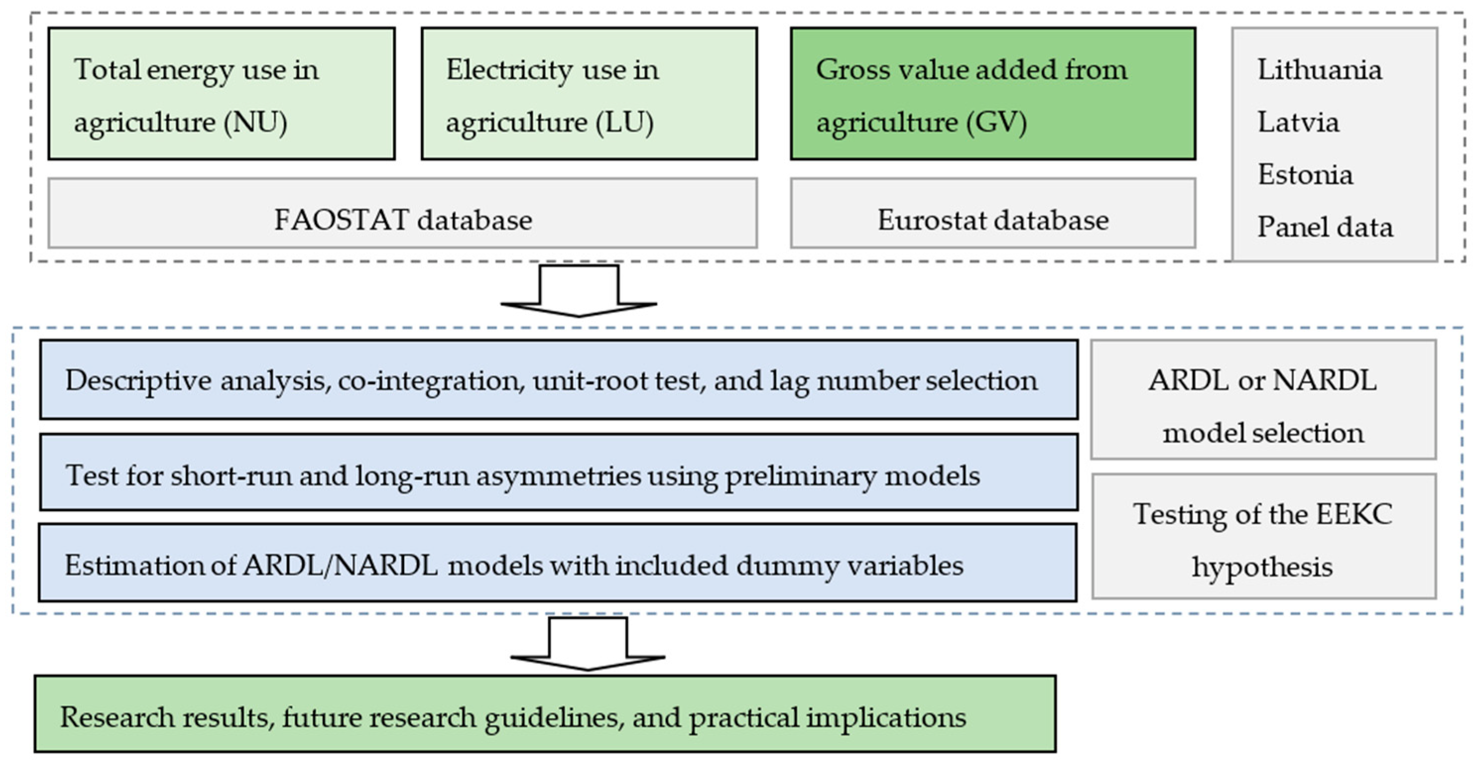
2.1. Data

The research investigates the hypothesis of the energy–environmental Kuznets curve (EEKC) in the Baltic nations’ agricultural industry. The research employs a number of energy consumption indicators as a proxy for climate change, pollution, and environmental degradation. It is electricity use (LU) and total energy use (NU) in agriculture that result from economic growth as measured by agriculture’s gross added value (GV). The research examines annual statistics from 1995 to 2019. The indicator of economic growth is gross value added. Eurostat databases are used to gather data on financial accounts. To compare the economic outcomes of various nations, the gross value added is analysed in purchasing power parities (PPP) at the current prices for each year. Food and Agriculture Organization (FAO) reports are used to gather data on energy use. The data in the database consists of agriculture, forestry, and fisheries (hereafter, it is referred to as agriculture). The data on energy use are given in terajoules.

2.2. Methods

The research tests the energy–environmental Kuznets curve (EEKC) hypothesis in the agriculture sector in the Baltic States.
The study analyses energy consumption as a factor affecting the development of the country’s economy as well as directly determining the quality of the environment. This variable is used to assess whether, at a certain point, energy consumption begins to decrease as gross value added increases. Slowing down or reducing energy consumption results in lower GHG emissions, which in turn slows down environmental degradation. The study focuses on the agricultural sector, and FAOSTAT provides sufficiently detailed data on energy consumption in this sector, disaggregated by energy sources (fossil fuels, electricity among others.). It made it possible to study the impact of two dependent variables (total energy consumption and consumption of electricity as a less polluting environmental source) on the quality of the environment and compare the obtained results. Since economic growth can be both a positive and a negative indicator and does not indicate the level of development at which energy consumption would slow down or start to decrease, the study chose the independent variable, the gross added value created in agriculture, to describe economic growth. It reflects both the income of the population employed in the sector and the applied technologies, so it can be used to model the impact of gross added value on the volume of energy use and its efficiency.
The research is divided into several steps: (1) all three states’ descriptive data for indicators are given and discussed; (2) the following time series data evaluation tests are run: Engle-Granger co-integration test; ADF test; (3) preliminary ARDL/NARDL modelling is performed to determine the best amount of time lag and whether there are any asymmetric relationships between energy use and gross value added; (4) final parameter values are estimated and research hypotheses are tested by selecting either ARDL or NARDL and adding dummy variables to test for structural breaks (if parameters of regression models change over time). Next, we provide the study’s research framework (see Figure 1).
The study investigates the energy–environmental Kuznets curve hypothesis that as gross added value grows over time, the growth rate of energy use slows, and, finally, the quantity of energy used decreases. It is accomplished via the use of ARDL modelling, which is similar to the error correction model (ECM) approach and is founded on an ordinary least square (OLS) model, but that is also suitable for time series that are non-stationary and have varied order of integration [61]. In this instance, energy use, the dependent variable, has a long-term effect and short-term effect parameters for their influences on the first-level difference in the ARDL model. Therefore, the ARDL model is a type of unconstrained ECM because all of the long-term relationship variables are defined but not bound:
Δ Y t = μ + ρ Y t 1 + θ X t 1 + i = 1 p a i Δ Y t 1 + i = 0 q 1 ω i Δ X t 1 + D + S + ε t ,
where Y is the dependent variable; X is the independent variable; μ , ρ , θ , a , ω are model parameters; D and S are dummy variables; εt is the residual error; Δ is the difference in the first order; i is the time lag; p is the number of time lags for differences in Y ; q is the number of time lags for differences in X ; and t is the time.
As indicated in the previous section, the main research issue gives asymmetries many emphases. In order to simulate nonlinearities, co-integration, and causality simultaneously, the non-linear NARDL model is utilised. The distributed lag non-linear autoregressive distributed lag (NARDL) is an error correction model with a single equation that incorporates short- and long-run nonlinearities by using partial sum decompositions of positive and negative changes in the explanatory variables [62]. Using partial sum decompositions of the independent variable, this method assesses the asymmetry inside the long-run equilibrium relationship in addition to the short-run dynamic coefficients. Consequently, the gross value added (GV) is divided into its positive and negative components, GV+ and GV. The long-run indicators are the sums of these components: G V t = i = 1 t Δ G V i and G V t + = i = 1 t Δ G V i + . Then, NARDL modelling is then performed where G V is X , or L U is Y :
Δ Y t = μ + ρ Y t 1 + θ + X t 1 + + θ X t 1 + i = 1 p a i Δ Y t 1 + i = 0 q 1 ( ω i + Δ X t 1 + + ω i Δ X t 1 ) + D + S + ε t ,
where Y is the dependent variable; X + is the sum of positive differences in the independent variable; X is the sum of negative differences in the independent variable; D and S are dummy variables; D and S are dummy variables; μ , ρ , θ + , θ , a, ω + , ω are model parameters; ε t is the residual error; Δ is the difference in the first order; i is the time lag; p is the number of time lags for differences in Y ; q is the number of time lags for differences in X ; and t is the time.
Before performing ARDL/NARDL modelling, it is also determined whether the data’s time series are suitable for this analysis; an ADF test [63] is performed to assess stationarity when using the model that includes and excludes a time trend, and an Engle-Granger co-integration test [64] is performed to determine whether these time series are co-integrated with each other.
Preliminary time series models are estimated to identify the best number of time lags (q and p), using the number of time lags that provide preliminary ARDL models with the lowest values of the information criteria values. As in research by other authors using AR models [22,65], we choose to use three information criteria: the Hannan-Quinn information criterion, the Akaike information criterion, and the Schwartz information criterion. Then we estimate what number of differences in Y (named by p) and what number of differences in X (named by q) provide the lowest values of these information criteria.
The models also incorporate dummy variables. The research employs two time dummy variables to depict major events in the economic progress of the Baltic nations. This is during 2009 (dummy variable named as D_2009), when the economic crisis hit, causing a drop in gross added value, and since 2004, when all three nations joined the EU (dummy variable named as S_2004).
Two additional statistical hypotheses are tested when the models are estimated: h1: ρ = θ = 0 and h2: ω 0 = ω 1 = ω 2 = 0 . The second hypothesis, h2, tests if the joint short-run effect of gross value added from all time lags is equal to zero. Some variables from the ARDL equation must be removed using the Wald test [66] based on the covariance matrix to test hypotheses.
The statistical reliability of the models, the p-values of the parameter estimates, the coefficient of determination R2, the test of the normal distribution of the residual errors, and the test of their stationarity and autoregressive heteroskedasticity (ARCH) are all evaluated when analysing the estimates of the models.
The following models are calculated using a Gretl 2019a software technique. Using the sequential elimination of variables from models, insignificant factors with p-values of less than 0.05 are eliminated, leaving only the most significant variables that best describe the dynamics of energy usage. The QLR test is used to examine if structural breaks persist when time dummy variables are removed from the models and shown to be statistically insignificant. The QLR test is a variant of the Chow test [67] that uses the highest F statistic generated when the Chow test is performed on all probable break dates within a specified range. The analysis determines the observation at which the most significant value of the F statistic occurs using the default cut of 15%. The likelihood of this structural rupture is evaluated using the chi-square asymptotic p-value. The crucial value for the QLR at 5% is then noticed.

3. Results

The time series descriptive statistics for all three countries are presented below (see Figure 2 and Table 1). The average total energy use (NU) in agriculture is highest in Latvia (5869.0) and lowest in Estonia (4258.0). On the other hand, the average electricity use (LU) in the considered period is the lowest in Latvia (592.29) and the highest in Estonia (774.75). Gross value added in agriculture (GV) is highest in Lithuania (mean is 1761.8) and least in Estonia (mean is 632.65). The variation in total energy use is the largest in Lithuania (25.63% of the mean) and the smallest in Latvia (8.85% of the mean). The variation in electricity use is also the largest in Lithuania (39.52% of the mean) and the smallest in Latvia (12.54% of the mean). The variation in gross value added created in agriculture is the largest in Estonia (29.06% of the mean) and the smallest in Lithuania (18.66% of the mean). The averages of changes in energy use are negative values except for Estonia when analysing the total energy use (here, the mean is 61.819). This shows that energy use decreased in most cases during the considered period.
Figure 2. Baltic States time series: (a) total energy use in agriculture (NU); (b) electricity use in agriculture (LU); (c) Gross value added generated by agriculture (GV). Source: authors’ calculations based on Eurostat [68] and FAOSTAT [69] data, 2022.
Energies 16 02114 g002
Below are the results of the ADF test (see Table 2). In most cases, time series are stationary and do not have a unit root, but only when analysed with first-level differences. Using first-level differences, the time series are stationary in all cases except for electricity use (LU) in Estonia. The time series of total energy use (NU) in Estonia and the time series of electricity use (LU) in Lithuania are stationary only when applying the test with a constant.
The results of the co-integration test show that the time series are mostly co-integrated with each other when analysing Latvian data (see Table 3). Lithuanian data are less co-integrated with each other; in all cases, p-values are higher than 0.05. When analysing Latvian data, the time series using first-level differences are co-integrated in all cases, but when applying absolute values, only the time series of gross value added (GV) and total energy use (LU) are co-integrated. In the case of Estonia, only the time series of first-level differences and the time series of electricity use (LU), but not the total energy use (NU), are co-integrated. The fact that the series are co-integrated with each other in some instances justifies the need to use ARDL models in further analysis.
Next, preliminary NARDL models are built to determine the optimal number of time lags (see Appendix A). Considering the minimum values of the information criteria, the appropriate number of time lags was selected for further analysis. When analysing Lithuanian data, it is chosen to apply two time lags of energy use (p = 2) and one time lag of gross value added (q = 1) in terms of both NU and LU. When analysing Latvian data and applying total energy use, it is chosen to apply two time lags for NU (p = 2) and one time lag for GV (q = 1). When analysing electricity use, it is chosen to apply one time lag for LU (p = 1) and three time lags for GV (q = 3). When analysing Estonian data and applying total energy use, it is chosen to apply two time lags for NU (p = 2) and three time lags for GV (q = 3). When analysing electricity use, it is chosen to apply two time lags for LU (p = 2) and one time lag for GV (q = 1). When analysing the panel data, two time lags of energy use (p = 2) and one time lag of gross added value (q = 1) are chosen for both NU and LU. Next, a preliminary NARDL model is constructed, and hypotheses are tested that the long-run and short-run effects are symmetrical (see Table 4). In the cases of both Lithuania and Estonia, the time effects are symmetrical when examining total energy use (NU). In the cases of Estonia and panel data, short-term asymmetries have been identified. This suggests that gross value added (GV) explains energy use in the short run but that this effect is asymmetric in nature. When examining electricity use (LU), the hypothesis that this relationship is symmetrical is accepted in all cases. In summary, it can be said that in all cases, the ARDL model will be applied for further analysis, except for Estonia and panel data, where the NARDL model will be applied but only when modelling total energy use (NU).
First of all, the parameter estimates of the ARDL models of the Lithuanian NU and LU models are analysed (see Table 5). Both NU (−1) and LU (−1) energy use are statistically significant (p-value < 0.05) and negative. It shows that as the level of energy use increases, the growth rate of energy use slows down. Analysing the NU model, it was also observed that the constant is positive and statistically significant. All other parameters, including time dummy variables, are statistically insignificant. The NU model explains the dynamics better than the LU model, with a higher R2 of 0.7621. The residual errors of both models are not normally distributed (p-value < 0.05), but they are stationary when applying the model without or with a trend. Residual errors are also characterised by statistically significant ARCH effects (p-value < 0.05). Models after the sequential elimination of insignificant variables are provided in the appendices (see Appendix B). In reduced models, the constants are statistically significant and positive in both models. In the NU model, changes in energy use with a two-year time lag ΔNU (−2) are also statistically significant and positive. When applying the NU model, its residual errors are normally distributed. The time dummy variables are removed from the model, the QLR test is performed, and the structural breaks for both models are found to be in the year 2000.
Next, the parameter estimates of the ARDL models of the Latvian NU and LU models are analysed (see Table 6). Only NU (−1) is statistically significant (p-value < 0.05) and negative. It shows that as the level of energy use increases, the growth rate of energy use slows down. Analysing the NU model, it was also observed that the constant is positive and statistically significant. GV (−1) is statistically significant in both models and positive, showing that as gross value increases, so does energy use. ΔGV (−1) is statistically significant in the LU model but has a negative parameter value. All other parameters, including time dummy variables, are statistically insignificant. The LU model explains the dynamics better than the NU model, with a higher R2 of 0.6333. Both models’ residual errors are normally distributed (p-value > 0.05), and they are stationary when applying the model without a trend. In addition, residual errors are not characterised by statistically significant ARCH effects (p-value > 0.05). Models after the sequential elimination of insignificant variables are provided in the appendices (see Appendix C). The NU model shows similar parameter estimates, except that GV (0) is positive here and statistically significant. In the LU model, the time dummy variable S_2004 is also statistically significant and has a negative sign, showing that electricity use in agriculture decreased after the country joined the EU. As the time dummy variables are removed from the model, the QLR test is performed, and the structural break for the NU model is found to be in the year 2005.
Next, the parameter estimates for the Estonian NU NARDL and LU ARDL models are analysed (see Table 7). Both NU (−1) and LU (−1) energy use are almost statistically significant (p-value is near 0.05) and negative. GV (−1) is only statistically significant in the NU model and has a positive sign. All other parameters, including time dummy variables, are statistically insignificant. The NU model explains the dynamics better than the LU model, with a higher R2 of 0.7203. The residual errors of both models are normally distributed (p-value < 0.05), and they are stationary in the NU model. Residual errors are also characterised by statistically significant ARCH effects in the LU model (p-value < 0.05). Models after the sequential elimination of insignificant variables are provided in the appendices (see Appendix D). In the NU model, ΔGV (−2) is almost statistically significant (p-value = 0.0679), showing short-run asymmetry and a negative sign. In the LU model, LU (−1) is statistically significant and has a negative sign, showing that electricity use moves at a decreasing rate in the long run. However, neither model has normally distributed residual errors or ARCH effects. The time dummy variables are removed from the model, the QLR test is performed, and the structural breaks for both models are found to be in 2002 when applying the NU model, but there is no statistically significant structural break (unexpected change in parameter values) when analysing the LU model.
Finally, the parameter estimates for the panel NU NARDL and LU ARDL models are analysed (see Table 8). Both NU (−1) and LU (−1) energy use are statistically significant (p-value < 0.05) and negative. It shows that as the level of energy use increases, the growth rate of energy use slows down. Constants are statistically significant and have positive signs in both models. All other parameters, including time dummy variables, are statistically insignificant. The LU model explains the dynamics better than the NU model, with a higher R2 of 0.3799. The residual errors of both models are not normally distributed (p-value < 0.05), and they are not stationary when applying the model without or with a trend. There are no tools to reduce and subsequently remove insignificant variables from panel data models.
In conclusion, ARDL and NARDL models can be used to examine how energy use and gross value added (GV) in agriculture in different states are related. The optimal number of time lags for each state’s model was chosen by estimating preliminary ARDL models and then determining at what time lags (p and q) the information criteria values were the smallest.

4. Discussion

4.1. Comparison with Previous Studies

The results of this study allow us to expand the already available field of knowledge on the topic of the relationship between economic growth and energy use. In the works of other authors on this topic, economic growth, its connections with environmental safety aspects, GHG emissions, and energy consumption levels are mostly explored. The studies focus mainly on the developed countries of the world [26,70], but recent studies also analyse more broadly the less developed countries [23,30,71]. Some studies analyse data from several countries together, such as the EU countries [72]; others focus on the EU agricultural sector [73]; panel studies are also conducted [47,74,75,76]. On the other hand, there are some studies that specifically analyse the Baltic countries in these aspects [76,77,78,79,80,81], studies that focus more on testing the energy–Kuznets curve hypothesis in the Baltic States [82], and studies that focus exclusively on Lithuania [83]. The EEKC curve hypothesis was used in this study, which has not yet been broadly used in studies by other authors. It, in turn, characterises better the relationship between environmental quality, energy consumption, and economic growth. For a long time, the Baltic countries were planned economic states that belonged to the USSR. For them, in 1990–1991, after the restoration of independence and in 2004, after becoming members of the EU, the economy began to grow rapidly, and the service sector developed, as is typical of post-industrial countries. The study failed to identify a statistically significant inverted “U” curve effect in the Baltic countries. This essentially supports the observation of other authors that this effect is characteristic of states with historically developed economies [33] (it is not characteristic of the Baltic countries).
Although other authors [82,83] have used similar methodologies in their work, this study used the latest data on the Baltic countries, specifically the agricultural sector, which has not yet been analysed. The contradictory nature of research results is determined by the level of development of countries, the possibilities of replacing fossil fuels with renewable energy sources, as well as the research methods used. In the Baltic countries, the importance of agriculture to the country’s economy (as measured by the gross added value created) is higher than on average in the EU countries. In the Baltic countries, the agricultural sector still employs a relatively large share of the employed, and the income level and development of the population in rural areas depend on this sector. Another important aspect is that the added value created in the agriculture of the Baltic countries has the potential to increase by increasing the efficiency of the resources used. The study also used several energy consumption indicators (total energy and electricity consumption) and analysed structural break points (the financial crisis period of 2009 and countries’ membership in the EU). Electricity consumption was analysed separately from total energy consumption, assuming that electricity consumption is less polluting. The research focuses on agriculture and allows for a better study of the interactions between the gross added value created in agriculture, as expressed by economic growth, and the energy consumption in agriculture. The main observations of the study can be divided into several groups:
First, the study identified cases where short-term changes in economic growth measured by gross value added increased total energy consumption and electricity consumption. The short-term effects of economic growth are more noticeable when analysing total energy consumption than electricity consumption. These effects were mainly observed when analysing data from Latvia and Estonia but not from Lithuania. Other authors who were testing both the Kuznets environmental curve hypothesis through the lenses of energy use or GHG emissions also found similar effects: that GDP growth mostly affects energy use in more developed countries [23,84] or that the gross value added from agriculture is insignificant in some countries [85]. Authors who have mainly used energy consumption [86,87] have emphasised such problematic aspects of agriculture that alternative resources gradually replace the volume of energy consumption. In addition, this study demonstrates that relations of an asymmetric nature were identified in the analysis of Estonian data. Other authors who applied the NARDL model observed such effects but found asymmetric relationships in long-term effects [88]. Some studies also focus on electricity consumption [47,89,90], emphasising that a large part of the electricity is produced from renewable resources.
Another important observation in this study is that energy consumption increases when moving at a decreasing rate. A negative long-term effect parameter (NU) of energy consumption was found to be statistically significant in all cases, with similar results obtained when analysing countries separately and using panel data. On the other hand, it was not established that the gross added value would have a statistically significant negative long-term effect parameter (GV) on energy consumption, so the environmental hypothesis of Kuznets’ inverted “U” curve cannot be fully accepted since it cannot be said that energy consumption would start to decrease after reaching a certain level. Other authors have also not always accepted or rejected the environmental Kuznets curve hypothesis for all states [88,91], as the hypothesis is mainly accepted in industrialised or developed countries [24,26]. When analysing data from the Baltic countries, other authors used different indicators, such as CO2, but rejected these links as well [78]. The energy–Kuznets curve hypothesis is accepted in the most developed economies but not in low- to middle-income countries [23,71]. According to Filippidis et al. [47], who analysed panel data from more than 200 countries in 2021, the inverted U-energy Kuznets hypothesis is accepted, and the relationship between renewables and economic growth is simply a U-shaped curve. In addition, an “N”-shaped energy–Kuznets curve is observed [48]. However, this hypothesis was rejected by other authors who tested the energy–Kuznets curves of the Baltic countries [82]. The results of the study show that it can be assumed that the economies of the Baltic countries jumped to a higher level of economic development, skipping some stages of economic development that the economies of Western Europe went through, due to the changes that occurred in the economies of Central and Eastern Europe during the period of economic transformation when moving from a planned to a market economy.
Furthermore, suspected structural breaks (unexpected changes in parameter values) are characterised by dummy time variables, showing the major impacts on the agricultural sector of the Baltic countries: as assessed in 2008, the crisis, which had a significant impact on the economies of all three Baltic countries, and the period since joining the EU in 2004, when the volume of subsidies in the agriculture of the Baltic countries increased, the structure of agricultural exports changed, among others. When assessing structural breaks and the influence of economic crises on the shape of the curve, statistically significant breaks were identified only when analysing Latvian data. The results of the study suggest that Latvia’s accession to the EU had a negative impact on electricity consumption in agriculture. No such relationships were observed when analysing the data from other countries. On the other hand, it was observed that an unexpected change in parameter values in the analysis of Lithuanian data could be around 2000, based on QLR test results. Other authors also observed similar statistically significant structural breaks or economic changes in countries where they tested the EKC hypothesis [92].

4.2. Proposals for Future Research

The study’s main limitation is that the data were used only from 1995 since only that much data is available for the Baltic countries. Other studies have used longer time series significantly, reaching as far back as the 1970s, which provides more flexibility in choosing the ARDL econometric models to be applied [88,93]. The study also found little success in identifying asymmetric relationships. The conventional ARDL model was chosen to be applied more often than the NARDL model, which was often used in the works of other authors [88,94,95]. Other authors were able to identify not only short-term but also long-term asymmetric relationships [88].
As more data become available, the study can be expanded to include new crises related to the global health crisis and the tense political situation after 2022. During this period, the prices of agricultural products rose rapidly, and the standard of living fell, which may have led to changes in the relationship between gross value added and energy consumption in agriculture. Therefore, more dummy variables could be included in the research models. Other authors have already analysed the post-2020 periods and identified such problematic aspects as asymmetric impacts, as the long-run impact of the positive shock on oil prices is not similar to the negative shock [94]. In the study, structural breaks could be more detailed by choosing separate breaking points for individual states. As shown by the results of the QLR test for Lithuanian data, typical changes occurred around 2000.
The study could be further expanded by using more indicators covering economic growth. Other authors have used different indicators: the implementation of technological innovations in agriculture [95,96], the importance of foreign investment and trade openness [97,98,99], economic development [1,30], government interventions, the extent of renewable energy use [84,100,101,102], and other factors influencing energy consumption [103,104].
More sophisticated methods may also be used in the study. For example, methods that other authors employed in their studies include the ARDL cumulative sum (CUSUM) test [105], the dynamic ARDL [106], the bootstrap ARDL [107], the Granger test [24,85], the panel regression model [23], multilevel mixed-effects models [82], and non-parametric analysis [24].

4.3. Practical Implications

The study analysed the three Baltic States due to their comparable agricultural structures, similar production conditions, and the fact that these countries apply the Common Agricultural Policy. The General Agricultural Policy 2023–2027, not only in the Baltic countries but also in all EU countries, will be more focused on sustainable solutions to environmental problems, which can reduce the amount of greenhouse gas emissions and contribute to the implementation obligations of the green course and net zero goals.
The study results showed that an inverted “U” could not be established, but in all three states, energy consumption moves at a decreasing rate as gross value added increases. On the one hand, either these countries have not yet reached a level of economic development that is characterised by declining energy consumption, or the countries did not previously have a developed industrial sector and a rich agricultural sector and immediately transitioned to a service economy, which is why there is no clear and sloping inverted “U” curve. On the other hand, it shows that economic growth alone is not enough to solve environmental problems. The findings suggest that the government should prioritise carbon reduction measures and implement such policies more effectively at the national level.
Other authors, following their research findings, suggest different measures to manage energy use and greenhouse gas emissions in agriculture. The economic openness and financial development of the country are emphasised [97,98,108]. Others emphasise the importance of renewable energy sources [109,110]. It is especially important as in the Baltic countries, renewable energy sources are still not widely used. The study results could serve the Baltic countries in setting indicative national goals for reducing energy consumption in agriculture and finding opportunities to switch to renewable energy and increase energy efficiency to reduce greenhouse gas emissions by 2050, neutralising the impact on the climate [3].

5. Conclusions

This study examines the relationship between energy consumption in agriculture and the gross value added in agriculture. The research aims to supplement the already-existing field of knowledge and better explain the formation of these connections. The study uses countries less analysed in the works of other authors, and the study analyses the annual data of all three Baltic countries together and separately from 1995 to 2019. Since all three countries have similar agricultural systems and environmental aspects, the research results are comparable and provide new insights. The research used not only the total energy consumption in agriculture but also the electricity consumption in agriculture, as well as focusing on the entry of countries into the EU and the impact of the economic crisis. More complex time series models, such as ARDL and NARDL, were used to model these relationships and test whether they take an inverse or asymmetric shape over time. The study analyses whether, as gross value added increases, energy consumption increases up to a certain level and then starts to decrease.
The study led to three major conclusions. First of all, energy consumption increases but moves at a decreasing rate. A negative long-term effect parameter (NU) was found to be statistically significant in all cases, and similar results were obtained when analysing countries separately and panel data. On the other hand, it was not established that added value would have a statistically significant negative long-term effect parameter (GV) on energy consumption, so the environmental hypothesis of Kuznets’ inverted “U” curve cannot be entirely accepted. The conclusion of the study is basically similar to the results obtained by other researchers. The originality of the research lies in the fact that the relationship between energy use and economic growth in agriculture is investigated, and ARDL and NARDL models are applied to compare energy use to electricity use. To our knowledge, such a study has not been carried out before in the agriculture of the Baltic countries. On the other hand, short-term changes in economic growth increase total energy consumption and electricity consumption in most cases. Short-term effects are more noticeable when analysing total energy consumption than electricity consumption. These effects were mainly observed when analysing data from Latvia and Estonia but not from Lithuania. In the analysis of Estonian data, relations of an asymmetric nature were identified. Moreover, when assessing structural breaks and the influence of economic crises on the shape of the curve, a statistically significant time dummy variable was identified only when analysing Latvian data. The results of the study suggest that Latvia’s accession to the EU had a negative impact on electricity consumption in agriculture. No such relationships were observed when analysing the data from other countries. On the other hand, it was observed that the structural break in the analysis of Lithuanian data could be around 2000. For Kuznets’ hypothesis to be true, the energy produced from fossil fuels must be replaced more rapidly by energy produced from renewable energy sources in agriculture. It could also be influenced by the advanced production technologies, innovations and modernisation used in the production of agricultural products.
The data used in the study goes back only to 1995, as only that much data were available for all three Baltic countries. Other studies, which mainly analysed the economies of developed countries, tested the Kuznets curve hypothesis with much longer data series, which led to more flexibility in applying econometric models. On the other hand, the study can be expanded with the availability of more data. New crises related to the global health crisis and the tense political situation after 2020 may be included in the study. During this period, the prices of agricultural products rose rapidly, and the standard of living fell, which may have led to changes in the relationship between economic growth and energy consumption in agriculture. Therefore, more dummy variables could be included in the research models. The study could include more countries and compare results between eastern and western European countries. The study can also use more indicators showing environmental aspects and pollution.
The results of the study have important practical suggestions for further policy-making for policy makers who want to make decisions about energy efficiency in order to improve the quality of the environment while ensuring economic growth.

Author Contributions

Conceptualisation, D.M. and A.J.S.; methodology, D.M. and A.J.S.; software, A.J.S.; validation, D.M. and A.J.S.; formal analysis, A.J.S.; investigation, A.J.S.; resources, D.M.; data curation, D.M. and A.J.S.; writing—original draft preparation, D.M. and A.J.S.; writing—review and editing, D.M., A.J.S., B.V. and G.G.-Z.; visualisation, D.M. and A.J.S.; supervision, D.M. and A.J.S.; funding acquisition, B.V. All authors have read and agreed to the published version of the manuscript.

Funding

This research received no external funding.

Data Availability Statement

Not applicable.

Conflicts of Interest

The authors declare no conflict of interest in the results.

Appendix A

Table A1. Information criteria for best time lag selection.
Information
Criteria
Schwarz CriterionAkaike CriterionHannan-Quinn Criterion
Time Lagq = 1q = 2q = 3q = 1q = 2q = 3q = 1q = 2q = 3
Using NU and GV:
p = 1347.3501353.1688341.3105339.4016342.9494329.3090341.4006345.5195332.1362
p = 2328.5817334.6953340.3131319.8534323.7848327.2206321.9095326.3550330.3048
Latvia
p = 1338.9816342.9144332.6672331.0332332.6950320.6657333.0322335.2652323.4929
p = 2328.7566332.6071335.7460320.0283321.6967322.6535322.0844324.2669325.7377
Estonia
p = 1363.8117368.5495353.2095355.8632358.3300341.2080357.8622360.9002344.0352
p = 2347.1741352.0053348.5405338.4458341.0949335.4480340.5019343.6650338.5322
Panel
p = 11059.2151066.4711020.8471043.5761046.364996.76091049.7811054.3411006.278
p = 21008.4191016.4391024.166990.9015994.5423997.8898997.82341003.1951008.273
Using LU and GV:
Lithuania
p = 1296.0494301.9561293.5428288.1009291.7367281.5414290.0999294.3068284.3686
p = 2286.9268291.7369296.6200278.1985280.8264283.5275280.2546283.3966286.6117
Latvia
p = 1242.1129241.2186235.3446234.1645230.9992223.3432236.1635233.5693226.1703
p = 2235.8228235.3802238.4298227.0944224.4697225.3373229.1506227.0399228.4215
Estonia
p = 1284.8172289.8978280.4342276.8688279.6784268.4327278.8678282.2486271.2599
p = 2274.6944277.2970280.5093265.9661266.3866267.4168268.0222268.9567270.5010
Panel
p = 1829.5992837.5174802.6740813.9605817.4105778.5878820.1649825.3876788.1054
p = 2796.4406803.4549806.0290778.9233781.5583779.7532785.8452790.2107790.1360
Source: authors’ calculations based on Eurostat [68] and FAOSTAT [69] data, 2022.

Appendix B

Table A2. ARDL estimations for Lithuania after eliminating insignificant variables.
VariableCoefficientp-ValueVariableCoefficientp-Value
Using NU and GV:Using LU and GV:
Constant1848.5800<0.0001Constant289.73100.0014
NU (−1)−0.4621<0.0001LU (−1)−0.42480.0003
ΔNU (−2)0.31260.0128
Auxiliary hypotheses:
h1: reject, p-value < 0.0001
Supplementary estimations, p-values:
A normality test: 0.3113
ADF test of residual (without trend): 0.7711
ADF test of residual (with trend): 0.9966
ARCH effect: 0.0201
R-squared: 0.6961
QLR test p-value: <0.0001, year: 2000
Auxiliary hypotheses:
h1: reject, p-value 0.0003
Supplementary estimations, p-values:
A normality test: <0.0001
ADF test of residual (without trend): <0.0001
ADF test of residual (with trend): <0.0001
ARCH effect: 0.0017
R-squared: 0.4852
QLR test p-value: <0.0001, year: 2000
Source: authors’ calculations based on Eurostat [68] and FAOSTAT [69] data, 2022.

Appendix C

Table A3. ARDL estimations for Latvia after eliminating insignificant variables.
VariableCoefficientp-ValueVariableCoefficientp-Value
Using NU and GV:Using LU and GV:
Constant2867.70000.0072Constant32.17940.6094
NU (−1)−0.69360.0045LU (−1)−0.28730.0195
GV (−1)1.16900.0113GV (−1)0.18840.0019
ΔGV (0)1.38210.0247ΔGV (0)−0.20730.0088
S_2004−57.31010.0398
Auxiliary hypotheses:
h1: reject, p-value 0.0152
h2: reject, p-value 0.0247
Supplementary estimations, p-values:
A normality test: 0.9794
ADF test of residual (without trend): 0.0908
ADF test of residual (with trend): 0.3766
ARCH effect: 0.5300
R-squared: 0.4639
QLR test p-value: 0.4771, year: 2005
Auxiliary hypotheses:
h1: reject, p-value 0.0052
h2: reject, p-value 0.0088
Supplementary estimations, p-values:
A normality test: 0.7476
ADF test of residual (without trend): 0.0028
ADF test of residual (with trend): 0.5953
ARCH effect: 0.4847
R-squared: 0.5189
QLR test p-value: 0.2251, year: 2007
Source: authors’ calculations based on Eurostat [68] and FAOSTAT [69] data, 2022.

Appendix D

Table A4. NARDL estimations for Estonia after eliminating insignificant variables.
VariableCoefficientp-ValueVariableCoefficientp-Value
Using NU and GV:Using LU and GV:
Constant−36.78420.7742Constant306.0140.0566
ΔGV− (−2)−2.83660.0679LU (−1)−0.42000.0454
Auxiliary hypotheses:
h2: accept, p-value 0.0679
Supplementary estimations, p-values:
A normality test: 0.0025
ADF test of residual (without trend): 0.0352
ADF test of residual (with trend): 0.4397
ARCH effect: 0.4523
R-squared: 0.1571
QLR test p-value: 0.0228, year: 2002
Auxiliary hypotheses:
h1: reject, p-value 0.0454
Supplementary estimations, p-values:
A normality test: 0.0059
ADF test of residual (without trend): 0.2522
ADF test of residual (with trend): 0.4491
ARCH effect: 0.1634
R-squared: 0.1855
QLR test p-value: 0.5210, year: 2000
Source: authors’ calculations based on Eurostat [68] and FAOSTAT [69] data, 2022.

References

  1. Destek, M.A.; Sarkodie, S.A. Investigation of environmental Kuznets curve for ecological footprint: The role of energy and financial development. Sci. Total Environ. 2019, 650, 2483–2489. [Google Scholar] [CrossRef]
  2. Ridzuan, N.H.A.M.; Marwan, N.F.; Khalid, N.; Ali, M.H.; Tseng, M.L. Effects of agriculture, renewable energy, and economic growth on carbon dioxide emissions: Evidence of the environmental Kuznets curve. Resour. Conserv. Recycl. 2020, 160, 104879. [Google Scholar] [CrossRef]
  3. Xu, Z.; Baloch, M.A.; Meng, F.; Zhang, J.; Mahmood, Z. Nexus between financial development and CO2 emissions in Saudi Arabia: Analyzing the role of globalization. Environ. Sci. Pollut. Res. 2018, 25, 28378–28390. [Google Scholar] [CrossRef]
  4. Shahbaz, M.; Shahzad, S.J.H.; Mahalik, M.K. Is globalization detrimental to CO2 emissions in Japan? New threshold analysis. Environ. Model. Assess. 2018, 23, 557–568. [Google Scholar] [CrossRef] [Green Version]
  5. Zafar, M.W.; Saud, S.; Hou, F. The impact of globalization and financial development on environmental quality: Evidence from selected countries in the Organization for Economic Co-operation and Development (OECD). Environ. Sci. Pollut. Res. 2019, 26, 13246–13262. [Google Scholar] [CrossRef]
  6. Khan, I.; Hou, F.; Le, H.P. The impact of natural resources, energy consumption, and population growth on environmental quality: Fresh evidence from the United States of America. Sci. Total Environ. 2021, 754, 142222. [Google Scholar] [CrossRef]
  7. Zhang, L.; Pang, J.; Chen, X.; Lu, Z. Carbon emissions, energy consumption and economic growth: Evidence from the agricultural sector of China’s main grain-producing areas. Sci. Total Environ. 2019, 665, 1017–1025. [Google Scholar] [CrossRef]
  8. Roser, M. The World’s Energy Problem. 2020. Available online: https://ourworldindata.org/worlds-energy-problem (accessed on 15 October 2022).
  9. Sarkodie, S.A.; Ozturk, I. Investigating the environmental Kuznets curve hypothesis in Kenya: A multivariate analysis. Renew. Sustain. Energy Rev. 2020, 117, 109481. [Google Scholar] [CrossRef]
  10. Proposal for a Directive of the European Parliament and of the Council on Energy Efficiency (Recast). COM/2021/558 Final. 021/0203(COD). Available online: https://eur-lex.europa.eu/legal-content/EN/TXT/?uri=CELEX%3A52021PC0558 (accessed on 15 October 2022).
  11. Ritchie, H.; Roser, M.; Rosado, P. CO2 and Greenhouse Gas Emissions. Published Online at OurWorldInData.org. 2020. Available online: https://ourworldindata.org/co2-and-other-greenhouse-gas-emissions (accessed on 2 November 2022).
  12. Our World in Data Based on Climate Analysis Indicators Tool (CAIT). OurWorldInData.org/co2-and-Other-Greenhouse-Gas-Emissions. Available online: https://ourworldindata.org/emissions-by-sector (accessed on 18 October 2022).
  13. U.S. Energy Information and Administration (EIA). International Energy Outlook 2016: With Projections to 2040. 2016. Available online: https://www.eia.gov/outlooks/ieo/pdf/0484(2016).pdf (accessed on 3 November 2022).
  14. Leonard, M.D.; Michaelides, E.E.; Michaelides, D.N. Energy storage needs for the substitution of fossil fuel power plants with renewables. Renew. Energy 2020, 145, 951–962. [Google Scholar] [CrossRef]
  15. Holechek, J.L.; Geli, H.M.; Sawalhah, M.N.; Valdez, R. A global assessment: Can renewable energy replace fossil fuels by 2050? Sustainability 2022, 14, 4792. [Google Scholar] [CrossRef]
  16. Ma, B.; Yu, Y. Industrial structure, energy-saving regulations and energy intensity: Evidence from Chinese cities. J. Clean. Prod. 2017, 141, 1539–1547. [Google Scholar] [CrossRef]
  17. Salim, R.; Yao, Y.; Chen, G.S. Does human capital matter for energy consumption in China? Energy Econ. 2017, 67, 49–59. [Google Scholar] [CrossRef]
  18. Kander, A.; Warde, P.; Henriques, S.T.; Nielsen, H.; Kulionis, V.; Hagen, S. International trade and energy intensity during European industrialization, 1870–1935. Ecol. Econ. 2017, 139, 33–44. [Google Scholar] [CrossRef]
  19. Beyene, S.D.; Aruga, K. Investigating the energy-environmental Kuznets curve under panel quantile regression: A global perspective. Environ. Sci. Pollut. Res. 2022, 30, 20527–20546. [Google Scholar]
  20. Communication from the Commission to the European Parliament and the Council. Energy Efficiency and Its Contribution to Energy Security and the 2030 Framework for Climate and Energy Policy; COM(2014) 520 Final. Available online: https://eur-lex.europa.eu/legal-content/EN/TXT/?uri=COM:2014:0520:FIN (accessed on 4 November 2022).
  21. Eurostat; European Commission. GDP and Main Components (Output, Expenditure and Income) [nama_10_gdp]. Available online: https://appsso.eurostat.ec.europa.eu/nui/show.do?dataset=nama_10_gdp&lang=en (accessed on 2 November 2022).
  22. Hundie, S.K.; Daksa, M.D. Does energy-environmental Kuznets curve hold for Ethiopia? The relationship between energy intensity and economic growth. J. Econ. Struct. 2019, 8, 21. [Google Scholar] [CrossRef]
  23. Aruga, K. Investigating the energy-environmental Kuznets Curve hypothesis for the Asia-Pacific region. Sustainability 2019, 11, 2395. [Google Scholar] [CrossRef] [Green Version]
  24. Shahbaz, M.; Shafiullah, M.; Khalid, U.; Song, M. A nonparametric analysis of energy environmental Kuznets Curve in Chinese Provinces. Energy Econ. 2020, 89, 104814. [Google Scholar] [CrossRef]
  25. Van Benthem, A.A. Energy leapfrogging. J. Assoc. Environ. Resour. Econ. 2015, 2, 93–132. [Google Scholar] [CrossRef]
  26. Chen, Q.; Taylor, D. Economic development and pollution emissions in Singapore: Evidence in support of the Environmental Kuznets Curve hypothesis and its implications for regional sustainability. J. Clean. Prod. 2020, 243, 118637. [Google Scholar] [CrossRef]
  27. Liu, M.; Ren, X.; Cheng, C.; Wang, Z. The role of globalization in CO2 emissions: A semi-parametric panel data analysis for G7. Sci. Total Environ. 2020, 718, 137379. [Google Scholar] [CrossRef]
  28. Assamoi, G.R.; Wang, S.; Liu, Y.; Gnangoin, T.B.Y.; Kassi, D.F.; Edjoukou, A.J.R. Dynamics between participation in global value chains and carbon dioxide emissions: Empirical evidence for selected Asian countries. Environ. Sci. Pollut. Res. 2020, 27, 16496–16506. [Google Scholar] [CrossRef]
  29. Dogan, E.; Inglesi-Lotz, R. The impact of economic structure to the environmental Kuznets curve (EKC) hypothesis: Evidence from European countries. Environ. Sci. Pollut. Res. 2020, 27, 12717–12724. [Google Scholar] [CrossRef] [PubMed]
  30. Shah, S.A.R.; Naqvi, S.A.A.; Nasreen, S.; Abbas, N. Associating drivers of economic development with environmental degradation: Fresh evidence from Western Asia and North African region. Ecol. Indic. 2021, 126, 107638. [Google Scholar] [CrossRef]
  31. Husnain, M.I.U.; Haider, A.; Khan, M.A. Does the environmental Kuznets curve reliably explain a developmental issue? Environ. Sci. Pollut. Res. 2021, 28, 11469–11485. [Google Scholar] [CrossRef] [PubMed]
  32. Chen, J.; Hu, T.E.; Van Tulder, R. Is the environmental Kuznets curve still valid: A perspective of wicked problems. Sustainability 2019, 11, 4747. [Google Scholar] [CrossRef] [Green Version]
  33. Yu, Z.; Ponce, P.; Irshad, A.U.R.; Tanveer, M.; Ponce, K.; Khan, A.R. Energy efficiency and Jevons’ paradox in OECD countries: Policy implications leading toward sustainable development. J. Pet. Explor. Prod. Technol. 2022, 12, 2967–2980. [Google Scholar] [CrossRef]
  34. Wang, X.; Zhang, T.; Nathwani, J.; Yang, F.; Shao, Q. Environmental regulation, technology innovation, and low carbon development: Revisiting the EKC Hypothesis, Porter Hypothesis, and Jevons’ Paradox in China’s iron & steel industry. Technol. Forecast. Soc. Chang. 2022, 176, 121471. [Google Scholar]
  35. Jevons, W.S. The Coal Question: An Inquiry Concerning the Progress of the Nation and the Probable Exhaustion of Our Coal-Mines; Macmillan and Company: London, UK, 1866. [Google Scholar]
  36. Trincado, E.; Sánchez-Bayón, A.; Vindel, J.M. The European Union Green Deal: Clean Energy Wellbeing Opportunities and the Risk of the Jevons Paradox. Energies 2021, 14, 4148. [Google Scholar] [CrossRef]
  37. Grossman, G.M.; Krueger, A.B. Environmental Impacts of a North American Free Trade Agreement; Working Paper No. 3914; National Bureau of Economic Research: Cambridge, MA, USA, 1991. [Google Scholar]
  38. Grossman, G.M.; Krueger, A.B. Economic growth and the environment. Q. J. Econ. 1995, 110, 353–377. [Google Scholar] [CrossRef] [Green Version]
  39. Beckerman, W. Economic growth and the environment: Whose growth? Whose environment? World Dev. 1992, 20, 481–496. [Google Scholar] [CrossRef]
  40. Panayotou, T. Empirical Tests and Policy Analysis of Environmental Degradation at Different Stages of Economic Development (No. 992927783402676); International Labour Organization: Geneva, Switzerland, 1993. [Google Scholar]
  41. Kraft, J.; Kraft, A. On the relationship between energy and GNP. J. Energy Dev. 1978, 3, 401–403. [Google Scholar]
  42. Tiba, S.; Omri, A. Literature Survey on the Relationships between Energy Variables, Environment and Economic Growth; University Library of Munich: Munich, Germany, 2016. [Google Scholar]
  43. Pablo-Romero, M.D.P.; De Jesús, J. Economic growth and energy consumption: The energy-environmental Kuznets curve for Latin America and the Caribbean. Renew. Sustain. Energy Rev. 2016, 60, 1343–1350. [Google Scholar] [CrossRef]
  44. Aboagye, S. The policy implications of the relationship between energy consumption, energy intensity and economic growth in Ghana. OPEC Energy Rev. 2017, 41, 344–363. [Google Scholar] [CrossRef]
  45. Bilgili, F.; Koçak, E.; Bulut, Ü.; Kuloğlu, A. The impact of urbanization on energy intensity: Panel data evidence considering cross-sectional dependence and heterogeneity. Energy 2017, 133, 242–256. [Google Scholar] [CrossRef]
  46. Zhang, Q.; Liao, H.; Hao, Y. Does one path fit all? An empirical study on the relationship between energy consumption and economic development for individual Chinese provinces. Energy 2018, 150, 527–543. [Google Scholar] [CrossRef]
  47. Filippidis, M.; Tzouvanas, P.; Chatziantoniou, I. Energy poverty through the lens of the energy-environmental Kuznets curve hypothesis. Energy Econ. 2021, 100, 105328. [Google Scholar] [CrossRef]
  48. Mahmood, H.; Alkhateeb, T.T.Y.; Tanveer, M.; Mahmoud, D.H. Testing the energy-environmental Kuznets curve hypothesis in the renewable and nonrenewable energy consumption models in Egypt. Int. J. Environ. Res. Public Health 2021, 18, 7334. [Google Scholar] [CrossRef]
  49. Apergis, N.; Payne, J.E. Energy consumption and economic growth in Central America: Evidence from a panel cointegration and error correction model. Energy Econ. 2009, 31, 211–216. [Google Scholar] [CrossRef]
  50. Ajmi, A.N.; Hammoudeh, S.; Nguyen, D.K.; Sato, J.R. On the relationships between CO2 emissions, energy consumption and income: The importance of time variation. Energy Econ. 2013, 49, 629–638. [Google Scholar] [CrossRef]
  51. Lise, W.; Van Montfort, K. Energy consumption and GDP in Turkey: Is there a cointegration relationship? Energy Econ. 2007, 29, 1166–1178. [Google Scholar] [CrossRef]
  52. Zhang, C.; Xu, J. Retesting the causality between energy consumption and GDP in China: Evidence from sectoral and regional analyses using dynamic panel data. Energy Econ. 2012, 34, 1782–1789. [Google Scholar] [CrossRef]
  53. Shahbaz, M.; Mallick, H.; Mahalik, M.K.; Sadorsky, P. The role of globalization on the recent evolution of energy demand in India: Implications for sustainable development. Energy Econ. 2016, 55, 52–68. [Google Scholar] [CrossRef] [Green Version]
  54. Hao, Y.; Zhu, L.; Ye, M. The dynamic relationship between energy consumption, investment and economic growth in China’s rural area: New evidence based on provincial panel data. Energy 2018, 154, 374–382. [Google Scholar] [CrossRef]
  55. Rahman, Z.; Khattak, S.I.; Ahmad, M.; Khan, A. A disaggregated-level analysis of the relationship among energy production, energy consumption and economic growth: Evidence from China. Energy 2020, 194, 116836. [Google Scholar] [CrossRef]
  56. Al-Mulali, U.; Saboori, B.; Ozturk, I. Investigating the environmental Kuznets curve hypothesis in Vietnam. Energy Policy 2015, 76, 123–131. [Google Scholar] [CrossRef]
  57. Dong, X.-Y.; Ran, Q.; Hao, Y. On the nonlinear relationship between energy consumption and economic development in China: New evidence from panel data threshold estimations. Qual. Quant. 2019, 53, 1837–1857. [Google Scholar] [CrossRef]
  58. Shahbaz, M.; Shafiullah, M.; Papavassiliou, V.G.; Hammoudeh, S. The CO2–growth nexus revisited: A nonparametric analysis for the G7 economies over nearly two centuries. Energy Econ. 2017, 65, 183–193. [Google Scholar] [CrossRef] [Green Version]
  59. Shahbaz, M.; Shafiullah, M.; Mahalik, M.K. The dynamics of financial development, globalisation, economic growth and life expectancy in sub-Saharan Africa. Aust. Econ. Pap. 2019, 58, 444–479. [Google Scholar] [CrossRef]
  60. Key Results of the 2020 Farm Structure Survey in Estonia, Latvia and Lithuania. In Results of the Agricultural Census 2020 (Edition 2022); Statistics Lithuania. Available online: https://osp.stat.gov.lt/zus2020-rezultatai/zemes-ukio-surasymo-pagrindiniai-rezultatai-estijoje-latvijoje-ir-lietuvoje (accessed on 4 November 2022).
  61. Pesaran, M.H.; Shin, Y.; Smith, R.J. Bounds testing approaches to the analysis of level relationships. J. Appl. Econom. 2001, 16, 289–326. [Google Scholar] [CrossRef]
  62. Shin, Y.; Yu, B.; Greenwood-Nimmo, M. Modelling asymmetric cointegration and dynamic multipliers in a nonlinear ARDL framework. In Festschrift in Honor of Peter Schmidt; Springer: New York, NY, USA, 2014; pp. 281–314. [Google Scholar]
  63. Said, S.E.; Dickey, D.A. Testing for unit roots in autoregressive-moving average models of unknown order. Biometrika 1984, 71, 599–607. [Google Scholar] [CrossRef]
  64. Engle, R.F.; Granger, C.W. Co-integration and error correction: Representation, estimation, and testing. Econom. J. Econom. Soc. 1987, 55, 251–276. [Google Scholar] [CrossRef]
  65. Ali, W.; Abdullah, A.; Azam, M. Re-visiting the environmental Kuznets curve hypothesis for Malaysia: Fresh evidence from ARDL bounds testing approach. Renew. Sustain. Energy Rev. 2017, 77, 990–1000. [Google Scholar] [CrossRef]
  66. Wald, A. Tests of statistical hypotheses concerning several parameters when the number of observations is large. Trans. Am. Math. Soc. 1943, 54, 426–482. [Google Scholar] [CrossRef]
  67. Chow, G.C. Tests of equality between sets of coefficients in two linear regressions. Econom. J. Econom. Soc. 1960, 28, 591–605. [Google Scholar] [CrossRef] [Green Version]
  68. Eurostat; European Commission. Gross Value Added and Income by A*10 Industry Breakdowns [nama_10_a10]. Available online: https://appsso.eurostat.ec.europa.eu/nui/submitViewTableAction.do (accessed on 9 September 2022).
  69. FAOSTAT. Energy Use. Available online: https://https://www.fao.org/faostat/en/#data/GN (accessed on 9 September 2022).
  70. Haider, A.; Rankaduwa, W.; ul Husnain, M.I.; Shaheen, F. Nexus between Agricultural Land Use, Economic Growth and N2O Emissions in Canada: Is There an Environmental Kuznets Curve? Sustainability 2022, 14, 8806. [Google Scholar] [CrossRef]
  71. Moosa, I.A.; Burns, K. The Energy Kuznets Curve: Evidence from Developed and Developing Economies. Energy J. 2022, 43, 47–70. [Google Scholar] [CrossRef]
  72. Baležentis, T.; Streimikiene, D.; Zhang, T.; Liobikiene, G. The role of bioenergy in greenhouse gas emission reduction in EU countries: An Environmental Kuznets Curve modelling. Resour. Conserv. Recycl. 2019, 142, 225–231. [Google Scholar] [CrossRef]
  73. Vlontzos, G.; Niavis, S.; Pardalos, P. Testing for Environmental Kuznets curve in the EU Agricultural Sector through an eco-(in) efficiency index. Energies 2017, 10, 1992. [Google Scholar] [CrossRef] [Green Version]
  74. Zoundi, Z. CO2 emissions, renewable energy and the Environmental Kuznets Curve, a panel cointegration approach. Renew. Sustain. Energy Rev. 2017, 72, 1067–1075. [Google Scholar] [CrossRef]
  75. He, P.; Ya, Q.; Chengfeng, L.; Yuan, Y.; Xiao, C. Nexus between environmental tax, economic growth, energy consumption, and carbon dioxide emissions: Evidence from China, Finland, and Malaysia based on a Panel ARDL approach. Emerg. Mark. Financ. Trade 2021, 57, 698–712. [Google Scholar] [CrossRef]
  76. Zortuk, M.; Çeken, S. Testing environmental Kuznets curve in the selected transition economies with panel smooth transition regression analysis. Amfiteatru Econ. J. 2016, 18, 537–547. [Google Scholar]
  77. Simionescu, M.; Wojciechowski, A.; Tomczyk, A.; Rabe, M. Revised environmental Kuznets curve for V4 countries and Baltic states. Energies 2021, 14, 3302. [Google Scholar] [CrossRef]
  78. Kar, A.K. Environmental Kuznets curve for CO2 emissions in Baltic countries: An empirical investigation. Environ. Sci. Pollut. Res. 2022, 29, 47189–47208. [Google Scholar] [CrossRef]
  79. Li, T.; Baležentis, T.; Makutėnienė, D.; Streimikiene, D.; Kriščiukaitienė, I. Energy-related CO2 emission in European Union agriculture: Driving forces and possibilities for reduction. Appl. Energy 2016, 180, 682–694. [Google Scholar] [CrossRef]
  80. Yan, Q.; Yin, J.; Baležentis, T.; Makutėnienė, D.; Štreimikienė, D. Energy-related GHG emission in agriculture of the European countries: An application of the Generalized Divisia Index. J. Clean. Prod. 2017, 164, 686–694. [Google Scholar] [CrossRef]
  81. Jóźwik, B.; Gavryshkiv, A.V.; Kyophilavong, P.; Gruszecki, L.E. Revisiting the environmental Kuznets curve hypothesis: A case of Central Europe. Energies 2021, 14, 3415. [Google Scholar] [CrossRef]
  82. Pablo-Romero Gil-Delgado, M.D.P.; Sánchez Braza, A. Residential energy environmental Kuznets curve in the EU-28. Energy 2017, 125, 44–54. [Google Scholar] [CrossRef]
  83. Rahman, H.U.; Ghazali, A.; Bhatti, G.A.; Khan, S.U. Role of economic growth, financial development, trade, energy and FDI in environmental Kuznets curve for Lithuania: Evidence from ARDL bounds testing approach. Eng. Econ. 2020, 31, 39–49. [Google Scholar] [CrossRef] [Green Version]
  84. Bekhet, H.A.; Othman, N.S. The role of renewable energy to validate dynamic interaction between CO2 emissions and GDP toward sustainable development in Malaysia. Energy Econ. 2018, 72, 47–61. [Google Scholar] [CrossRef]
  85. Ali, S.; Ying, L.; Shah, T.; Tariq, A.; Ali Chandio, A.; Ali, I. Analysis of the nexus of CO2 emissions, economic growth, land under cereal crops and agriculture value-added in Pakistan using an ARDL approach. Energies 2019, 12, 4590. [Google Scholar] [CrossRef] [Green Version]
  86. Khan, M.K.; Khan, M.I.; Rehan, M. The relationship between energy consumption, economic growth and carbon dioxide emissions in Pakistan. Financ. Innov. 2020, 6, 1. [Google Scholar] [CrossRef] [Green Version]
  87. Tong, T.; Ortiz, J.; Xu, C.; Li, F. Economic growth, energy consumption, and carbon dioxide emissions in the E7 countries: A bootstrap ARDL bound test. Energy Sustain. Soc. 2020, 10, 20. [Google Scholar] [CrossRef]
  88. Zafeiriou, E.; Mallidis, I.; Galanopoulos, K.; Arabatzis, G. Greenhouse gas emissions and economic performance in EU agriculture: An empirical study in a non-linear framework. Sustainability 2018, 10, 3837. [Google Scholar] [CrossRef] [Green Version]
  89. Saint Akadiri, S.; Alola, A.A.; Olasehinde-Williams, G.; Etokakpan, M.U. The role of electricity consumption, globalization and economic growth in carbon dioxide emissions and its implications for environmental sustainability targets. Sci. Total Environ. 2020, 708, 134653. [Google Scholar] [CrossRef]
  90. Borozan, D. Efficiency of energy taxes and the validity of the residential electricity environmental Kuznets curve in the European Union. Sustainability 2018, 10, 2464. [Google Scholar] [CrossRef] [Green Version]
  91. Özokcu, S.; Özdemir, Ö. Economic growth, energy, and environmental Kuznets curve. Renew. Sustain. Energy Rev. 2017, 72, 639–647. [Google Scholar] [CrossRef]
  92. Pata, U.K. Renewable energy consumption, urbanization, financial development, income and CO2 emissions in Turkey: Testing EKC hypothesis with structural breaks. J. Clean. Prod. 2018, 187, 770–779. [Google Scholar] [CrossRef]
  93. Ali, M.U.; Gong, Z.; Ali, M.U.; Wu, X.; Yao, C. Fossil energy consumption, economic development, inward FDI impact on CO2 emissions in Pakistan: Testing EKC hypothesis through ARDL model. Int. J. Financ. Econ. 2021, 26, 3210–3221. [Google Scholar] [CrossRef]
  94. Aljadani, A.; Toumi, H.; Toumi, S.; Hsini, M.; Jallali, B. Investigation of the N-shaped environmental Kuznets curve for COVID-19 mitigation in the KSA. Environ. Sci. Pollut. Res. 2021, 28, 29681–29700. [Google Scholar] [CrossRef]
  95. Zeraibi, A.; Balsalobre-Lorente, D.; Shehzad, K. Examining the asymmetric nexus between energy consumption, technological innovation, and economic growth; Does energy consumption and technology boost economic development? Sustainability 2020, 12, 8867. [Google Scholar] [CrossRef]
  96. Balsalobre-Lorente, D.; Shahbaz, M.; Chiappetta Jabbour, C.J.; Driha, O.M. The role of energy innovation and corruption in carbon emissions: Evidence based on the EKC hypothesis. In Energy and Environmental Strategies in the Era of Globalization; Springer: Cham, Switzerland, 2019; pp. 271–304. [Google Scholar]
  97. Ghazouani, T.; Boukhatem, J.; Sam, C.Y. Causal interactions between trade openness, renewable electricity consumption, and economic growth in Asia-Pacific countries: Fresh evidence from a bootstrap ARDL approach. Renew. Sustain. Energy Rev. 2020, 133, 110094. [Google Scholar] [CrossRef]
  98. Hasson, A.; Masih, M. Energy Consumption, Trade Openness, Economic Growth, Carbon Dioxide Emissions and Electricity Consumption: Evidence from South Africa Based on ARDL. 2017. Available online: https://mpra.ub.uni-muenchen.de/79424/ (accessed on 9 April 2022).
  99. Van Chien, N. Energy consumption, income, trading openness, and environmental pollution: Testing environmental Kuznets curve hypothesis. J. Southwest Jiaotong Univ. 2020, 55. [Google Scholar] [CrossRef]
  100. Chen, Y.; Wang, Z.; Zhong, Z. CO2 emissions, economic growth, renewable and non-renewable energy production and foreign trade in China. Renew. Energy 2019, 131, 208–216. [Google Scholar] [CrossRef]
  101. Yao, S.; Zhang, S.; Zhang, X. Renewable energy, carbon emission and economic growth: A revised environmental Kuznets Curve perspective. J. Clean. Prod. 2019, 235, 1338–1352. [Google Scholar] [CrossRef]
  102. Zhang, J.; Alharthi, M.; Abbas, Q.; Li, W.; Mohsin, M.; Jamal, K.; Taghizadeh-Hesary, F. Reassessing the Environmental Kuznets Curve in relation to energy efficiency and economic growth. Sustainability 2020, 12, 8346. [Google Scholar] [CrossRef]
  103. Jun, J. Relationship between Energy Consumption and Tourism in Latin America and the Caribbean: The Application of the Environmental Kuznets Curve. Lat. Am. Stud. Rev. 2017, 8, 3–28. [Google Scholar]
  104. Mahmood, H.; Maalel, N.; Hassan, M.S. Probing the Energy-Environmental Kuznets Curve hypothesis in oil and natural gas consumption models considering urbanization and financial development in Middle East countries. Energies 2021, 14, 3178. [Google Scholar] [CrossRef]
  105. Latif, A.; Javed, R. Does economic growth, population growth and energy use impact carbon-dioxide emissions in Pakistan? An ARDL approach. Bull. Bus. Econ. 2021, 10, 85–91. [Google Scholar]
  106. Khan, M.K.; Teng, J.Z.; Khan, M.I. Effect of energy consumption and economic growth on carbon dioxide emissions in Pakistan with dynamic ARDL simulations approach. Environ. Sci. Pollut. Res. 2019, 26, 23480–23490. [Google Scholar] [CrossRef]
  107. Pata, U.K.; Aydin, M. Testing the EKC hypothesis for the top six hydropower energy-consuming countries: Evidence from Fourier Bootstrap ARDL procedure. J. Clean. Prod. 2020, 264, 121699. [Google Scholar] [CrossRef]
  108. Naqvi, S.A.A.; Shah, S.A.R.; Anwar, S.; Raza, H. Renewable energy, economic development, and ecological footprint nexus: Fresh evidence of renewable energy environment Kuznets curve (RKC) from income groups. Environ. Sci. Pollut. Res. 2021, 28, 2031–2051. [Google Scholar] [CrossRef]
  109. Dong, K.; Sun, R.; Jiang, H.; Zeng, X. CO2 emissions, economic growth, and the environmental Kuznets curve in China: What roles can nuclear energy and renewable energy play? J. Clean. Prod. 2018, 196, 51–63. [Google Scholar] [CrossRef]
  110. Zambrano-Monserrate, M.A.; Silva-Zambrano, C.A.; Davalos-Penafiel, J.L.; Zambrano-Monserrate, A.; Ruano, M.A. Testing environmental Kuznets curve hypothesis in Peru: The role of renewable electricity, petroleum and dry natural gas. Renew. Sustain. Energy Rev. 2018, 82, 4170–4178. [Google Scholar] [CrossRef]
Figure 1. The study’s research framework.
Energies 16 02114 g001
Table 1. Descriptive statistics of total energy use by agriculture (NU), electricity use by agriculture (LU), and gross value added generated by agriculture (GV).
IndicatorLithuaniaLatviaEstonia
NULUGVNULUGVNULUGV
Using initial value LU, NU, and GV:
Mean4307.7806.431761.85869.0592.29995.894258.0774.75632.65
Median3998.9702.001732.75904.8583.20964.904271.1748.80628.85
Minimum3513.9597.601097.45071.6486.00541.102086.4565.20341.30
Maximum8098.91803.62300.06770.1741.601658.45636.71227.6922.20
Standard deviation1104.0318.72328.80519.3874.287274.39911.93135.45183.85
Standard deviation, %25.6339.5218.668.8512.5427.5521.4217.4829.06
Skewness2.40632.2518−0.10190.01670.32520.4071−0.69301.5051−0.0544
Kurtosis4.82913.5790−0.9646−0.9212−0.9454−0.03110.26173.4275−1.2993
Using differences of variables ∆NU, ∆LU and ∆GV:
Mean−171.53−45.42020.625−3.3928−8.310031.57961.819−31.35020.458
Median−22.250−12.6004.8500−16.513−1.80007.550084.350−12.60041.700
Minimum−2014.1−676.80−591.10−933.15−158.40−161.80−1297.0−338.40−294.70
Maximum413.5054.000385.30820.8457.600256.901702.3126.00271.10
Standard deviation538.75152.79251.12392.4450.284113.69593.90107.49126.98
Skewness−2.0762−3.2051−0.2809−0.1506−1.20290.28210.2617−1.4470−0.4026
Kurtosis4.321310.495−0.22590.39541.5072−0.99831.66942.40720.2846
Mean−171.53−45.42020.625−3.3928−8.310031.57961.819−31.35020.458
Source: authors’ calculations based on Eurostat [68] and FAOSTAT [69] data, 2022.
Table 2. Augmented Dickey–Fuller test results.
IndicatorLithuaniaLatviaEstonia
NULUGVNULUGVNULUGV
Using initial values LU, NU and GV, p-values:
test without trend0.03450.00170.41170.3590.37970.99110.55130.13910.2725
test with trend0.21650.91820.93230.33740.72590.12410.05930.20960.1693
Using differences of variables ∆NU, ∆LU and ∆GV, p-values:
test without trend0.00230.01010.00030.00230.00120.00160.04170.1902<0.0001
test with trend0.00160.22360.00430.01440.01560.01940.09420.3326<0.0001
Source: authors’ calculations based on Eurostat [68] and FAOSTAT [69] data, 2022.
Table 3. Engle–Granger co-integration test results.
IndicatorLithuaniaLatviaEstonia
NULUNULUNULU
Using initial values LU, NU and GV, p-values:
test without trend0.15920.09890.04640.74060.23040.3236
test with trend0.55300.44280.18950.80000.24470.7029
Using differences of variables ∆NU, ∆LU and ∆GV, p-values:
test without trend0.39840.18920.01400.03460.08050.0023
test with trend0.69880.15350.04360.05260.21080.0172
Source: authors’ calculations based on Eurostat [68] and FAOSTAT [69] data, 2022.
Table 4. Results of tests for long- and short-run symmetry.
Time PeriodLong Run,
p-Value
Short Run,
p-Value
Conclusion
Using NU and GV:
Lithuania0.80710.5781No asymmetry
Latvia0.72850.5901No asymmetry
Estonia0.22770.0511Short-run asymmetry
All Baltic States0.91350.0605Short-run asymmetry
Using LU and GV:
Lithuania0.24500.7645No asymmetry
Latvia0.22260.5955No asymmetry
Estonia0.67290.4765No asymmetry
All Baltic States0.59220.5577No asymmetry
Source: authors’ calculations based on Eurostat [68] and FAOSTAT [69] data, 2022.
Table 5. Autoregressive distributed lag (ARDL) estimations for Lithuania.
VariableCoefficientp-ValueVariableCoefficientp-Value
Using NU and GV:Using LU and GV:
Constant1836.86000.0078Constant29.77190.8978
NU (−1)−0.40460.0020LU (−1)−0.41820.0147
GV (−1)−0.18880.5496GV (−1)0.13230.3130
ΔNU (−1)−0.05540.7337ΔLU (−1)−0.14240.5091
ΔNU (−2)0.32600.0611ΔLU (−2)−0.00640.9768
ΔGV (0)0.14740.7384ΔGV (0)0.09850.5898
S_2004150.51000.5680S_200424.20270.8294
D_2009−461.02900.3123D_200925.66390.8896
Auxiliary hypotheses:
h1: reject, p-value 0.0028
h2: accept, p-value 0.7384
Supplementary estimations, p-values:
A normality test: 0.0294
ADF test of residual (without trend): <0.0001
ADF test of residual (with trend): 0.1416
ARCH effect: 0.0069
R-squared: 0.7621
Auxiliary hypotheses:
h1: reject, p-value 0.0453
h2: accept, p-value 0.5898
Supplementary estimations, p-values:
A normality test: <0.0001
ADF test of residual (without trend): 0.0666
ADF test of residual (with trend): 0.0003
ARCH effect: 0.0006
R-squared: 0.5563
Source: authors’ calculations based on Eurostat [68] and FAOSTAT [69] data, 2022.
Table 6. Autoregressive distributed lag (ARDL) estimations for Latvia.
VariableCoefficientp-ValueVariableCoefficientp-Value
Using NU and GV:Using LU and GV:
Constant3822.09000.0068Constant51.39000.4677
NU (−1)−0.87150.0034LU (−1)−0.27360.0574
GV (−1)1.17560.0358GV (−1)0.15620.0257
ΔNU (−1)0.02780.8851ΔLU (−1)0.08530.6659
ΔNU (−2)0.06020.7623ΔGV (0)−0.05000.4712
ΔGV (0)1.08930.1233ΔGV (−1)−0.20670.0211
S_2004149.95300.5260ΔGV (−2)0.07770.3146
D_2009−554.49300.1354S_2004−46.53060.1262
D_2009−61.00390.0935
Auxiliary hypotheses:
h1: reject, p-value 0.0106
h2: accept, p-value 0.1233
Supplementary estimations, p-values:
A normality test: 0.8378
ADF test of residual (without trend): 0.0001
ADF test of residual (with trend): 0.6360
ARCH effect: 0.5394
R-squared: 0.5608
Auxiliary hypotheses:
h1: accept, p-value 0.0597
h2: reject, p-value 0.0322
Supplementary estimations, p-values:
A normality test: 0.1525
ADF test of residual (without trend): 0.0002
ADF test of residual (with trend): 0.2104
ARCH effect: 0.6933
R-squared: 0.6333
Source: authors’ calculations based on Eurostat [68] and FAOSTAT [69] data, 2022.
Table 7. Non-linear autoregressive distributed lag (NARDL) estimations for Estonia.
VariableCoefficientp-ValueVariableCoefficientp-Value
Using NU and GV:Using LU and GV:
Constant967.87900.3635Constant454.43300.1450
NU (−1)−0.56590.0556LU (−1)−0.54740.0813
GV (−1)3.58000.0279GV (−1)−0.14550.5428
ΔNU (−1)0.24520.2689ΔLU (−1)−0.19070.4072
ΔNU (−2)0.25020.2985ΔLU (−2)−0.28340.3253
ΔGV+ (0)−1.76860.3538ΔGV (0)−0.08800.7304
ΔGV+ (−1)−2.97270.1935S_200452.18980.5847
ΔGV+ (−2)−3.51180.1361D_2009−118.20600.3424
ΔGV− (0)6.17390.0618
ΔGV− (−1)−0.42140.8167
ΔGV− (−2)−2.40540.2168
S_20041247.94000.2461
D_2009−302.64800.6116
Auxiliary hypotheses:
h1: reject, p-value 0.0295
h2: accept, p-value 0.0861
Supplementary estimations, p-values:
A normality test: 0.3319
ADF test of residual (without trend): 0.0011
ADF test of residual (with trend): <0.0001
ARCH effect: 0.3966
R-squared: 0.7203
Auxiliary hypotheses:
h1: accept, p-value 0.2049
h2: accept, p-value 0.7304
Supplementary estimations, p-values:
A normality test: 0.0732
ADF test of residual (without trend): 0.0694
ADF test of residual (with trend): 0.2552
ARCH effect: 0.0109
R-squared: 0.3297
Source: authors’ calculations based on Eurostat [68] and FAOSTAT [69] data, 2022.
Table 8. Non-linear autoregressive distributed lag (NARDL) estimations for panel data of all three Baltic countries.
VariableCoefficientp-ValueVariableCoefficientp-Value
Using NU and GV:Using LU and GV:
Constant833.87700.0046Constant191.21300.0024
NU (−1)−0.14510.0122LU (−1)−0.3244<0.0001
GV (−1)−0.27400.1597GV (−1)−0.00010.9967
ΔNU (−1)0.14290.2109ΔLU (−1)−0.09080.3841
ΔNU (−2)0.10000.3739ΔLU (−2)0.02040.8590
ΔGV+ (0)0.13070.6001ΔGV (0)0.02620.7307
ΔGV− (0)0.01130.9735S_200428.01080.4087
S_2004105.85000.5649D_2009−45.15880.4546
D_2009−318.88500.2711
Auxiliary hypotheses:
h1: reject, p-value 0.0065
h2: accept, p-value 0.7343
Supplementary estimations, p-values:
A normality test: <0.0001
ADF test of residual (without trend): 0.3296
ADF test of residual (with trend): 0.8198
R-squared: 0.2496
Auxiliary hypotheses:
h1: reject, p-value < 0.0001
h2: accept, p-value 0.7307
Supplementary estimations, p-values:
A normality test: <0.0001
ADF test of residual (without trend): 0.3739
ADF test of residual (with trend): 0.1441
R-squared: 0.3799
Source: authors’ calculations based on Eurostat [68] and FAOSTAT [69] data, 2022.
Disclaimer/Publisher’s Note: The statements, opinions and data contained in all publications are solely those of the individual author(s) and contributor(s) and not of MDPI and/or the editor(s). MDPI and/or the editor(s) disclaim responsibility for any injury to people or property resulting from any ideas, methods, instructions or products referred to in the content.

