Assessment of the Thermodynamic and Numerical Modeling of LES of Multi-Component Jet Mixing at High Pressure

Abstract

Mixing under high pressure conditions plays a central role in several engineering applications, such as direct-injection engines and liquid rocket engines. Numerical flow simulations have become a complementary tool to study the mixing process under these conditions but require complex thermodynamic modeling as well as validation with accurate experimental data. For this reason, we use experiments of supercritical single-phase jet mixing from the literature, where the mixing is quantified by the mixture speed of sound, as a reference for our work. We here focus on the thermodynamic modeling of multi-component flows under high pressure conditions and the analytical calculation of the mixture speed of sound. Our thermodynamic model is based on cubic equations of state extended for multi-components. Using an extension of OpenFOAM, we perform large-eddy simulations of hexane and pentane injections and compare our results with the experimentally measured mixture speed of sound at specific positions. The simulation results show the same characteristic trends, indicating that the mixing effects are well reproduced in the simulations. Additionally, the effect of the sub-grid scale modeling is assessed by comparing results using different models (Smagorinsky, Vreman, and Wall-Adapting Local Eddy-viscosity). The comprehensive simulation data presented here, in combination with the experimental data, provide a benchmark for numerical simulations of jet mixing in high pressure conditions.

1. Introduction

Mixing at high pressure conditions plays a central role in several engineering applications. Examples include direct-injection engines [1,2] and liquid-propellant rocket engines [3]. High pressure and temperature conditions as well as limited optical access can make experimental measurements challenging. For this reason, numerical flow simulations have become an essential tool for the development of future liquid-propellant rocket engines and internal combustion engines, complementing experimental investigations. By providing high-resolution, three-dimensional flow field data, numerical flow simulations can allow deeper insights into the underlying physics and enable detailed investigation of specific aspects. However, the validation of such simulation tools is an essential first step. To this end, detailed and quantitative experimental flow field data of different configurations and at well-defined conditions is required. In addition, the quantitatively measured variable has to be accessible in the simulations, and its correlation and background have to be well understood.

The first investigations of jet mixing at high pressure conditions were based on experimental studies. Quantitative data of jet mixing was measured using laser-based spectroscopic techniques, such as Raman scattering and laser-induced fluorescence. Mayer et al. [4] conducted Raman scattering measurements in cryogenic nitrogen jets discharged into nitrogen at sub- and supercritical temperatures. They measured the density decay in the axial direction and radial profiles at selected axial positions. Later, Oschwald et al. [5] performed quantitative density field measurements using Raman scattering in coaxial liquid nitrogen/gaseous hydrogen jets. Recently, Klima et al. [6] employed an enhanced Raman scattering methodology to quantitatively study ethanol/air-mixtures. Using laser-induced fluorescence, Roy and Segal [7] and Roy et al. [8] examined the planar density fields of the jet mixing zones of supercritical fluoroketone injections. An alternative experimental measurement technique is laser-induced thermal acoustics (LITA) [9]. Recently, Baab et al. [10] performed LITA measurements to provide a comprehensive speed of sound database for binary jet mixing zones at high pressure conditions. They examined the mixing for five different configurations with well-defined experimental conditions, considering the injection of hexane, pentane (two different injection temperatures), and fluoroketone (two different chamber pressures). To obtain an insight into both the axial decay and the transversal mixing, the quantitative speed of sound values were measured along the jet center line and in the radial direction.

As mentioned in the beginning, numerical simulations have become an essential complementary tool for the design of future engines. These investigations include Reynolds-Averaged-Navier–Stokes (RANS) studies [11,12], most commonly transient large-eddy simulations (LES) (e.g., [13,14,15,16,17]), and a few examples of computationally expensive direct numerical simulations (DNS) [18,19,20]. For validation against experimental data, a realistic turbulent inflow profile at the nozzle outlet is essential, since it affects the jet characteristics [21,22,23,24]. To this end, either the injector flow can be included in the simulations [25], a separate precursor LES of a pipe flow can be conducted [16,26], or a synthetic inflow generator [20,27], such as the one by Klein et al. [28], can be employed. Another aspect of LES studies of trans- and supercritical flows represents the sub-grid scale modeling. Since common modeling approaches were originally developed for incompressible flows, their suitability for investigations at supercritical pressures and with complex real gas thermodynamics cannot be generally assumed [29]. For example, Müller et al. [16,26] and Petit et al. [30] studied the effect of different sub-grid scale models on LES simulations of nitrogen injections [4] and co-axial injections [5,31,32]. In addition to this, another important aspect for numerical simulations is the thermodynamic modeling. To capture the complex thermodynamics, particularly the non-linear behavior around the critical point, sophisticated thermodynamic modeling approaches are required. An approach commonly used in early [30,33,34,35] as well as recent studies [13,14,15,16,20,36,37] is the employment of a thermodynamic model based on a cubic equation of state (EoS). Moreover, theoretical models for the transport properties are necessary, with the correlations by Chung et al. [38] being commonly employed (e.g., [13,14,15,16,17,39]). An alternative approach to an EoS-based framework is the usage of tabulated thermodynamic reference data [25,40]. In general, all these thermodynamic frameworks have evolved from single-component systems to multi-component systems, where non-linear mixing rules [41,42] are required to reproduce the highly non-ideal mixture properties, to multi-component systems including phase separation [14,15,43].

Numerical studies performing a quantitative comparison with experimental data can be summarized as follows. Numerous research groups [17,26,30,34,44,45,46,47] have performed simulations of cryogenic nitrogen injection at supercritical pressure following the experiments of Mayer et al. [4]. Binary systems, such as coaxial nitrogen/hydrogen injections [5], have been studied numerically, by e.g., Müller et al. [16] and Jafari et al. [47]. More recently, Traxinger [12], Jafari et al. [27] and Föll et al. [48] studied the hexane injection case of Baab et al. [10]. Mixing processes with phase separation effects have been considered in several recent studies [13,15,25] quantitatively comparing the liquid and vapor penetration lengths with experimental data.

In the present work, we aim to further exploit the data by Baab et al. [10] and to use them for more extensive comparisons. To this end, we first examine the characteristics of the mixture speed of sound and its analytical evaluation. Then, we present LES simulation results of hexane and pentane injections covering three of the five documented configurations. We validate our modeling approach by comparing the axial and radial profiles with the experimental data. Furthermore, we also evaluate the effects of the sub-grid scale modeling on the simulation results and compare the results with the experimental data. Based on the findings of previous studies [26,30], we consider the Smagorinsky [49], the Vreman [50], and the WALE [51] model, extending the previous studies by another validation case. Moreover, the mixture speed of sound and the distribution of the mass fraction in the simulation results are analyzed in detail. In our LES studies, we use an extension of OpenFOAM, specifically adapted for real gas simulations and successfully validated for high pressure injections [12,16,26]. The employed thermodynamic model is based on a cubic EoS extended for multi-component configurations. The digital filter-based inflow generator [28] is employed to provide turbulent inflow data.

The paper is structured as follows. The numerical method and thermodynamic model are presented in Section 2. Section 3 presents the considered configuration and the numerical setup. Results are analyzed in Section 4, where we first assess the thermodynamic modeling. Then, the simulation results are compared with experimental data. Afterwards, the effect of the sub-grid scale model is studied, and at the end, more detailed analyses of the simulation results are conducted. Section 5 summarizes the paper.

2. Mathematical and Physical Model

This section presents the mathematical and physical models. The governing equations are the Navier–Stokes equations (see Section 2.1), and the thermodynamic modeling is based on a homogeneous mixture model combined with a multi-component cubic equation of state (EoS) (see Section 2.2 and Section 2.3). For the sub-grid scale modeling, eddy-viscosity models are employed (see Section 2.5).

2.1. Governing Equations

We consider the three-dimensional, compressible Navier–Stokes equations for mass

$$\frac{\partial \rho }{\partial t}+\frac{\partial \left(\rho u_i\right)}{\partial x_i}=0,$$

(1)

momentum

$$\frac{\partial \left(\rho u_i\right)}{\partial t}+\frac{\partial \left(\rho u_i{u}_j\right)}{\partial x_j}=-\frac{\partial p}{\partial x_i}+\frac{\partial {\tau }_{ij}}{\partial x_j},$$

(2)

and energy conservation

$$\frac{\partial \left(\rho h\right)}{\partial t}+\frac{\partial \rho u_{i}h}{\partial x_i}=\frac{\partial p}{\partial t}+u_i\frac{\partial p}{\partial x_i}-\frac{\partial q_i}{\partial x_i},$$

(3)

where $\rho$, $u_i$, p, and h denote the density, velocity, pressure, and enthalpy. The viscous stress tensor ${\tau }_{ij}$ is calculated using Stokes’ hypothesis

$${\tau }_{ij}=2\mu \left(S_{ij}-\frac{1}{3}{\delta }_{ij}{S}_{kk}\right),$$

(4)

where $\mu$ is the dynamic viscosity, $S_{ij}$ the deformation tensor

$$S_{ij}=\frac{1}{2}\left(\frac{\partial u_i}{\partial x_j}+\frac{\partial u_j}{\partial x_i}\right),$$

(5)

and ${\delta }_{ij}$ the Kronecker Delta, which is 1 if $i=j$ and 0 if $i\ne j$. The heat transfer $q_i$ is modeled by Fourier’s law. Neglecting pressure gradients, $q_i$ can be approximated by [12]

$$\begin{array}{cc}\hfill q_i& =-\frac{\lambda }{c_p}\frac{\partial h}{\partial x_i},\hfill \end{array}$$

(6)

where $\lambda$ denotes the heat conductivity and $c_p$ the heat capacity at constant pressure.

Using the single-fluid approach [52], the governing Equations (1)–(3) are considered for a mixture fluid defined by the mixture quantities within a computational cell. For each additional species, a transport equation for the mass fraction Y is solved

$$\frac{\partial \left(\rho Y_k\right)}{\partial t}+\frac{\partial \left(\rho u_i{Y}_k\right)}{\partial x_i}=-\frac{\partial j_{k,i}}{\partial x_i}.$$

(7)

Since we consider a two-component mixture, we solve only one additional transport equation for the mass fraction. The diffusion of species k in i-th direction $j_{k,i}$ is described by Fick’s law

$$j_{k,i}=-\rho D_D\frac{\partial Y_k}{\partial x_i}.$$

(8)

The diffusion coefficient $D_D$ is modeled species independent and here obtained from the heat diffusivity assuming a constant Lewis number $Le=\lambda /\left(D_D{c}_p\rho \right)=1$ following Zips et al. [53] and Traxinger [12]. Yao et al. [54] studied the influence of different diffusion models on the prediction of single-phase instabilities in high pressure flames and observed no significant effects.

The governing equations are closed using an EoS and expressions for the heat capacity and enthalpy (see Section 2.2) together with constitutive relations for the transport properties (see Section 2.3).

2.2. Thermodynamic Model

The cubic equation of state by Peng–Robinson (PR) [55], extended for multi-component mixtures, describes the relation of the pressure, density, temperature, and molar composition. All other quantities are derived using the departure function formalism. The transport properties viscosity $\mu$ and heat conductivity $\lambda$ are calculated with the correlations by Chung et al. [38]. A detailed description of the employed thermodynamic model can be found in Trummler et al. [56].

2.2.1. Generalized Cubic Equation of State

We here consider the generalized formulation of a cubic EoS [57]

$$p(\underline{v},T)=\frac{RT}{\underline{v}-b}-\frac{a\alpha }{(\underline{v}+{\delta }_{1}b)(\underline{v}+{\delta }_{2}b)},$$

(9)

where the pressure p is a function of the molar volume $\underline{v}$ and the temperature T. R denotes the universal gas constant with $R=8314.472\mathrm{J}/\left(\mathrm{kmol}\mathrm{K}\right)$; ${\delta }_1$ and ${\delta }_2$ are additional EoS parameters for the generalized form and are constants for the PR EoS, having the values ${\delta }_1=1+\sqrt{2}$ and ${\delta }_2=1-\sqrt{2}$. The traditional EoS parameter are $a\alpha$ and b, where a represents the attractive forces and reads for the PR EoS

$$a=0.45724\left(\frac{R^2{T}_c^2}{p_c}\right)$$

(10)

with $T_c$ and $p_c$ being the critical temperature and the critical pressure; a is multiplied by a temperature dependent correction factor

$$\begin{array}{c}\hfill \alpha ={\left(1+\kappa (1-\sqrt{T/T_c})\right)}^2,\end{array}$$

(11)

where $\kappa$ is a function of the acentric factor $\omega$

$$\begin{array}{c}\hfill \kappa =0.37464+1.54226\omega -0.26992{\omega }^2.\end{array}$$

(12)

Then, b represents the repulsive forces and reads for the PR EoS

$$b=0.0778\left(\frac{R{T}_c}{p_c}\right).$$

(13)

To solve the cubic EoS (Equation (9)), the equation is reformulated using the dimensionless compressibility factor $Z=p\underline{v}/\left(RT\right)$. Details on solving cubic EoS can be found in the literature [13,15,39,56,58].

Besides the correlation provided by the EoS, expressions for thermodynamic properties internal energy e, entropy s, enthalpy h, and specific heats $c_p$ and $c_v$ are needed for the numerical flow simulations. These quantities are evaluated using the departure function formalism [59,60]. The formulations presented here are obtained from Matheis [39] and reformulated for the generalized cubic EoS.

For the internal energy e, this reads

$$e(\underline{v},T)=e_0\left(T\right)+{\int }_{\infty }^{\underline{v}}\left(T\frac{\partial p}{\partial T}{|}_{\underline{v}}-p\right)\mathrm{d}\underline{v},$$

(14)

where the subscript 0 denotes the ideal reference state. Solving the integral yields

$$e-e_0=\left(a\alpha -T\frac{\partial a\alpha }{\partial T}\right)K,$$

(15)

with

$$K=\frac{1}{b({\delta }_1-{\delta }_2)}ln\left(\frac{\underline{v}+{\delta }_{1}b}{\underline{v}+{\delta }_{2}b}\right).$$

(16)

Thus, the enthalpy h

$$h-h_0=e-e_0+p\underline{v}-RT$$

(17)

can be evaluated with

$$\begin{array}{c}\hfill h-h_0=\left(a\alpha -T\frac{\partial a\alpha }{\partial T}\right)K+p\underline{v}-RT.\end{array}$$

(18)

The correlation for the heat capacity at constant volume $c_v$ reads

$$(c_v-c_{v0})=-T\frac{{\partial }^{2}a\alpha }{\partial T^2}K,$$

(19)

where $c_{v0}$ is evaluated using $c_{v0}=c_{p0}-R$, and $c_{p0}$ denotes the heat capacity at constant pressure at ideal reference state and is determined with the seven-coefficient NASA polynomials using the values provided by Goos et al. [61]. Then, the heat capacity at constant pressure $c_p$ can be determined using

$$c_p=c_v-T{\left(\frac{\partial p}{\partial T}{|}_{\underline{v}}\right)}^2/\frac{\partial p}{\partial \underline{v}}{|}_{{}_T},$$

(20)

with

$$\frac{\partial p}{\partial T}{|}_{\underline{v}}=\frac{R}{\underline{v}-b}+\frac{\partial a\alpha }{\partial T}\frac{1}{N}$$

(21)

and

$$\frac{\partial p}{\partial \underline{v}}{|}_T=-\frac{RT}{{(\underline{v}-b)}^2}+\frac{a\alpha (2\underline{v}+({\delta }_1+{\delta }_2)b)}{N^2},$$

(22)

with the denominator

$$N=(\underline{v}+{\delta }_{1}b)(\underline{v}+{\delta }_{2}b)={\underline{v}}^2+({\delta }_1+{\delta }_2)b\underline{v}+{\delta }_1{\delta }_2{b}^2.$$

(23)

Finally, the speed of sound c can be evaluated using Equations (19), (20) and (22)

$$c=\sqrt{\frac{c_p}{c_v}\frac{\partial p}{\partial \underline{v}}{|}_{{}_T}\frac{{\underline{v}}^2}{M}}.$$

(24)

2.2.2. Multi-Component Modeling

For multi-component mixtures, the EoS parameters $a\alpha$ and b in Equation (9) are calculated as a function of the molar composition, represented by the molar fraction $z_i$. Following conventional mixing rules [41], they are determined as follows

$$a\alpha =\sum _i^{N_c}\sum _j^{N_c}{z}_i{z}_j{a}_{ij}{\alpha }_{ij},$$

(25)

$$b=\sum _i^{N_c}{z}_i{b}_i.$$

(26)

The coefficients $a_{ij}$ and ${\alpha }_{ij}$ are evaluated with the pseudo-critical mixing rules [42], where both are evaluated according to Equations (10) and (11) using the pseudo-critical quantities

$$\begin{array}{cc}\hfill & T_{c,ij}=\sqrt{T_{c,i}{T}_{c,j}}(1-k_{ij}),\hfill \\ \hfill & Z_{c,ij}=0.5(Z_{c,i}+Z_{c,j}),\hfill \\ \hfill & v_{c,ij}=\frac{1}{8}{\left[v_{c,i}^{1/3}+v_{c,j}^{1/3}\right]}^3,\hfill \\ \hfill & p_{c,ij}=Z_{c,ij}(R{T}_{c,ij}/v_{c,ij}),\hfill \\ \hfill & {\omega }_{ij}=0.5({\omega }_i+{\omega }_j).\hfill \end{array}$$

(27)

$k_{ij}$ is the binary interaction parameter and assumed to be $k_{ij}=0$. Thus, $a_{ij}$ and ${\alpha }_{ij}$ are calculated as follows

$$a_{ij}=0.45724\left(\frac{R^2{T}_{c,ij}^2}{p_{c,ij}}\right)$$

(28)

and

$$\begin{array}{c}\hfill {\alpha }_{ij}={\left(1+{\kappa }_{ij}(1-\sqrt{T/T_{c,ij}})\right)}^2\end{array}$$

(29)

with

$$\begin{array}{c}\hfill {\kappa }_{ij}=0.37464+1.54226{\omega }_{ij}-0.26992{\omega }_{ij}^2.\end{array}$$

(30)

The thermodynamic properties of the mixture are calculated as described in Section 2.2.1 using the EoS parameters of the mixture Equations (25) and (26). Hence, the mixture speed of sound is evaluated with Equation (24) inserting the properties and derivatives of the mixture.

2.3. Transport Properties Viscosity and Heat Conductivity with the Chung Correlations

For numerical flow simulations, suitable relations for the transport properties viscosity $\mu$ and heat conductivity $\lambda$ are required. The correlations by Chung et al. [38] are often used for real gas simulations [13,14,15,16,17,39]. For a detailed description of the model, we refer to Chung et al. [38] and Poling et al. [59] and provide only a brief description in the following. $\mu$ and $\lambda$ are calculated with

$$\mu ={\mu }_k+{\mu }_p\mathrm{and}\lambda ={\lambda }_k+{\lambda }_p,$$

(31)

where ${\mu }_k$ and ${\lambda }_k$ dominate at low pressures and are based on the Chapman–Enskog theory for diluted gases; ${\mu }_p$ and ${\lambda }_p$ dominate at higher pressures and are based on empirical correlations. The input for the model is composed of the temperature, the density, and the heat capacity $c_v$, where the latter only affects the evaluation of $\lambda$.

2.4. Numerical Method and Flow Solver

The finite volume method is used to solve the governing equations (Equations (1)–(3) and (7)). For spatial discretization, second-order centered differences are employed. The time integration is performed with a second-order implicit backward scheme.

For the simulations in this work, an in-house extension of the flow solver OpenFOAM by the Institute for Thermodynamics at the Bundeswehr University Munich is used. In it, the pressure-based framework in OpenFOAM is adapted following Issa [62,63] to be applicable to weakly compressible flows, where Jarczyk and Pfitzner [64] modified the algorithm to be applicable to real gas flow simulations using cubic EoS. Müller et al. [16,26] successfully validated this extended OpenFOAM framework for injections at high pressure conditions. Recently, the solver has been extended to supersonic flows [65,66,67]. A detailed description of this OpenFOAM extension can be found in the literature [12,68].

The pressure equation is solved with the PIMPLE algorithm, combining the Semi-Implicit Method for Pressure Linked Equations (SIMPLE) algorithm of Patankar and Spalding [69] and the Pressure-Implicit with Splitting of Operators (PISO) algorithm by Issa et al. [70].

2.5. Sub-Grid Scale Modeling

In LES, the smallest turbulent flow scales are not resolved on the computational grid. Thus, the effects of these unresolved sub-grid scales must be modeled to correctly represent the physical energy cascade process. We use an explicit LES approach relying on the eddy-viscosity concept. Favre filtering of the governing equations (Equations (1)–(3) and (7)) yields the sub-grid scale fluxes ${\tau }_{ij}^{SGS}$, $q_i^{SGS}$ and $j_{k,i}^{SGS}$ in the filtered momentum, energy, and transport equation, which have to be modeled. To this end, the following correlations are employed

$${\tau }_{ij}^{SGS}=-2{\mu }^{SGS}\left({\tilde{S}}_{ij}-\frac{1}{3}\widetilde{S_{kk}}{\delta }_{ij}\right)$$

(32)

$$q_i^{SGS}=-\frac{{\mu }^{SGS}}{P{r}_t}\frac{\partial \tilde{h}}{\partial x_i}$$

(33)

and

$$j_{k,i}^{SGS}=-\frac{{\mu }^{SGS}}{S{c}_t}\frac{\partial {\tilde{Y}}_k}{\partial x_i},$$

(34)

where $\tilde{\star }=\overline{\rho \star }/\overline{\rho }$ and $\overline{\star }$ denote the Favre averaging and finite volume averaging, respectively. For the sub-grid scale heat and mass fluxes, the turbulent Prandtl number ($P{r}_t$) and the turbulent Schmidt number ($S{c}_t$) are assumed constant. Although this assumption of a constant turbulent Prandtl number is widely used, it should be taken with caution, especially for wall-bounded flows including heat transfer [40,71]. Following previous studies of similar configurations, we set $P{r}_t=1$ [12,14,16,26] and $S{c}_t=1$ [12,14,16]. For the modeling of the sub-grid scale viscosity ${\mu }^{SGS}$, we employ three different well-established models. Mainly, we use the Wall-Adapting Local Eddy-viscosity (WALE) model [51], where ${\mu }^{SGS}$ is modeled with

$${\mu }^{SGS}=\overline{\rho }{(C_W\Delta )}^2\frac{{\left({\tilde{S}}_{ij}^d{\tilde{S}}_{ij}^d\right)}^{2/3}}{{\left({\tilde{S}}_{ij}{\tilde{S}}_{ij}\right)}^{5/2}+{\left({\tilde{S}}_{ij}^d{\tilde{S}}_{ij}^d\right)}^{5/4}}.$$

(35)

$C_W$ denotes the model constant, which is set to $C_W=0.325$ using the default parameter, and $\Delta$ is the filter size. ${\tilde{S}}_{ij}^d$ denotes the traceless symmetric part of the square of the velocity gradient tensor

$${\tilde{S}}_{ij}^d=\frac{1}{2}({\tilde{g}}_{ij}^2+{\tilde{g}}_{ji}^2)-\frac{1}{3}{\tilde{g}}_{kk}^2{\delta }_{ij}\mathrm{with}{\tilde{g}}_{ij}=\frac{\partial {\tilde{u}}_i}{\partial x_j}.$$

(36)

The WALE model has been specifically designed to return the correct asymptotic wall behavior for wall-bounded flows but also showed good modeling capabilities for various configurations, including compressible flows with phase transition [24,72]. The choice of the WALE model for most of the presented simulations has also been motivated by the fact that Koukouvinis et al. [25] have recently successfully employed it for simulations of transcritical injections with phase transition (ECN spray A).

In addition to the WALE model, we also conduct comparative studies with the well-known Smagorinsky model [49] and the Vreman model [50]. For the Smagorinsky model [49], the modeling of ${\mu }^{SGS}$ reads

$${\mu }^{SGS}=\overline{\rho }{(C_S\Delta )}^2\sqrt{2{\tilde{S}}_{ij}{\tilde{S}}_{ij}}.$$

(37)

The model constant $C_S=0.17$ has been used following Traxinger [12]. Several previous LES studies of high pressure injections employed the Smagorinsky model (e.g., [12,26,35,47]).

Vreman [50] proposed the following correlation

$${\mu }^{SGS}=\overline{\rho }{C}_V\sqrt{\frac{B_{\beta }}{{\alpha }_{ij}{\alpha }_{ij}}}$$

(38)

with

$$B_{\beta }={\beta }_{11}{\beta }_{22}+{\beta }_{11}{\beta }_{33}+{\beta }_{22}{\beta }_{33}-{\beta }_{12}^2-{\beta }_{13}^2-{\beta }_{23}^2,$$

(39)

$${\beta }_{ij}={\Delta }^2{\alpha }_{ki}{\alpha }_{kj}\mathrm{and}{\alpha }_{ij}=\frac{\partial {\tilde{u}}_j}{\partial x_i}.$$

(40)

The model constant $C_V$ has been set to $C_V=2.5C_S^2$ [50], where $C_S$ is the model constant from the Smagorinsky model. For example, Müller et al. [16,26] used the Vreman model for trans- and supercritical flows.

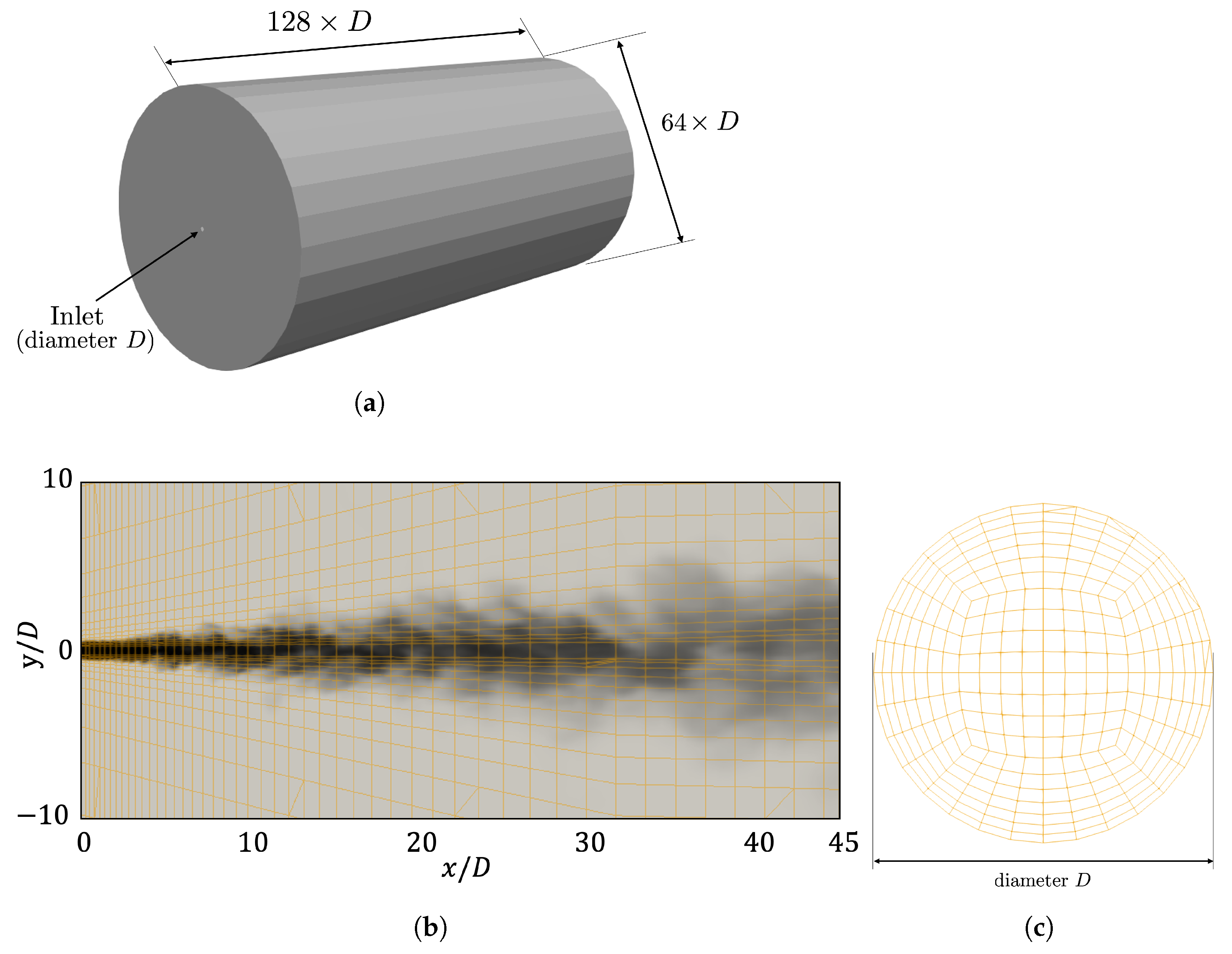
3. Considered Configurations and Numerical Setup

Our numerical setup is based on the experiments by Baab et al. [10], where various hot fluids ($T_e\approx 600\mathrm{K}$) were injected into a chamber filled with nitrogen at room temperature ($T_{ch}=296\mathrm{K}$) and at supercritical pressure with respect to the pure components. The injector nozzle is a straight single-hole injector with a diameter of $D=0.236\mathrm{mm}$ and a length of $L_{\mathrm{Nozzle}}=0.8\mathrm{mm}(L_{\mathrm{Nozzle}}/D\approx 3.4)$. Using laser-induced thermal acoustics (LITA), the mixture speed of sound at selected axial and radial positions has been determined.

We consider three selected cases listed in

Table 1. Considered configurations. $T_{ch}$, p, $T_e$, $u_e$, and $R{e}_D$ denote the chamber temperature, the chamber pressure, the temperature and the mean velocity at the nozzle exit, and the Reynolds number.

Case	Fluid	${\mathit{T}}_{\mathit{ch}}$ $\left[\mathbf{K}\right]$	p $\left[\mathbf{MPa}\right]$	${\mathit{T}}_{\mathit{e}}$ $\left[\mathbf{K}\right]$	${\mathit{u}}_{\mathit{e}}$ $[\mathbf{m}/\mathbf{s}]$	${\mathit{Re}}_{\mathit{D}}$
$SoS$_1	$C_6{H}_{14}$	296	$4.99$	627	91	1.31 × 105
$SoS$_2	$C_5{H}_{12}$	296	$5.00$	597	96	1.22 × 105
$SoS$_3	$C_5{H}_{12}$	296	$5.00$	526	76	1.35 × 105

. The first case, SoS_1, refers to the injection of hexane ($C_6{H}_{14}$). The second and third cases, SoS_2 and SoS_3, are the injections of pentane ($C_5{H}_{12}$) at different injection temperatures.

Table 2. Critical properties obtained from Coolprop [73].

		${\mathit{p}}_{\mathit{c}}$ $\left[\mathbf{MPa}\right]$	${\mathit{T}}_{\mathit{c}}$ $\left[\mathbf{K}\right]$
Hexane	$C_6{H}_{14}$	3.04	507.82
Pentane	$C_5{H}_{12}$	3.37	469.70
Nitrogen	$N_2$	3.40	126.19

lists the critical properties of the pure components. It can be seen that the pressure in the chamber is supercritical with respect to the pure components.

For the considered configuration, the dimensionless Reynolds number is of relevance. The Reynolds number describes the ratio of inertial forces to viscous forces

$$Re=\frac{uL}{\nu },$$

(41)

where u, L, and $\nu$ denote a representative velocity, a representative length scale, and the kinematic viscosity $\nu =\mu /\rho$. Injection processes can be characterized by the Reynolds number

$$R{e}_D=\frac{\rho {\overline{u}}_{e}D}{\mu }$$

(42)

evaluated with the nozzle diameter D, the mean velocity at the nozzle exit ${\overline{u}}_e$, the density of the injected fluid $\rho$, and the dynamic viscosity of the injected fluid $\mu$. In the simulated cases (see Table 1), the Reynolds number $R{e}_D$ is at the order of $O\left({10}^5\right)$, indicating turbulent injection processes.

For compressible flows, the Mach number

$$Ma=\frac{u}{c}$$

(43)

is also of relevance, setting the velocity u in relation to the speed of sound c. The Mach number evaluated with the mean velocity at the nozzle exit and the speed of sound at injection condition is $Ma\approx 0.3$, and therefore the considered configurations are subsonic dense jets.

Figure 1 depicts the domain and the grid of our simulations. We simulate the outflow region after a round nozzle with a diameter of $D=0.236\mathrm{mm}$, following the corresponding experimental study [10]. To this end, we consider a cylindrical domain with a diameter of $64\times D$ and length of $128\times D$, see Figure 1a. The domain is discretized with a structured grid. Figure 1b shows the grid on the midplane overlaid to simulation results and Figure 1c the grid resolution in the nozzle cross section. The grid has a high resolution in the near nozzle region and the region of the jet mixing layer and then a smooth stretching in the outwards direction. The simulation results presented in this work have been obtained on a grid with 45 cells over the diameter, corresponding to a cell width of $\Delta x=5.24e-6\mathrm{m}$ and a resolution of about $\Delta x/\eta \approx 20$ at the nozzle outlet; $\eta$ denotes the Kolmogorov length scale $\eta \approx L_{t}R{e}^{-3/4}$, which is estimated using the turbulent Reynolds number $R{e}_t=u^{\prime }{L}_t/\nu$ [74]. The velocity fluctuations $u^{\prime }$ as well as the turbulent length scale $L_t$ are obtained from the inflow data. The grid resolution of about $20\Delta x/\eta$ is well-suited for LES studies and in the range of previous LES studies [75]. This grid resolution yields 3.8 × 10⁶ cells for the whole domain. In addition to this justification of the grid resolution, we have conducted a grid convergence study, shown in Figure 2. To this end, simulations of case SoS_1 on three different grid resolutions have been performed and compared. The statistics were obtained over approximately 10 flow-through times of the relevant near nozzle region ($x/D<40$). Figure 2 shows that the mean density in axial direction does not change significantly between the medium and the fine grid resolution, which indicates convergence. Moreover, we refer to previous numerical investigations [12] that also demonstrated grid convergence for the used resolution for a configuration resembling case SoS_1.

The boundary conditions are chosen as follows: At the inlet, a turbulent inflow is prescribed using the digital filter-based inflow generator by Klein et al. [28]. The OpenFOAM implementation of Immer [76] is employed to filter the random inlet data at specified grid points to obtain coherent, turbulent structures. In the present study, a turbulence intensity of $4\%$ has been chosen, which is comparable to the value used in previous numerical investigations of liquid jets [77] and supercritical jets [27]. The turbulent length scale $L_t$ is set to $L_t=1/6D$. At the walls and the front plate, no-slip conditions are prescribed. The domain outlet is modeled as a pressure outlet.

The domain is initialized with nitrogen at chamber conditions. At the inlet, the injected fluid at injection conditions is prescribed. A grid sequencing strategy is applied to reduce the computational cost. This means that for each case, we let the flow field first develop on a coarser grid and then refine the grid over several refinement levels to the final grid resolution. After the flow field has completely developed, the statistical sampling is started. Statistical data have been averaged over approximately 10 flow-through times of the relevant near nozzle region ($x/D<40$).

4. Results

In this section, we first present a detailed assessment of the thermodynamic modeling in Section 4.1. Then, in Section 4.2 and Section 4.3, the simulation results of the three selected operating points are compared with experimental data. The results using different sub-grid scale models are compared in Section 4.4. At the end of this section (Section 4.5), more detailed analyses of the simulation results are presented.

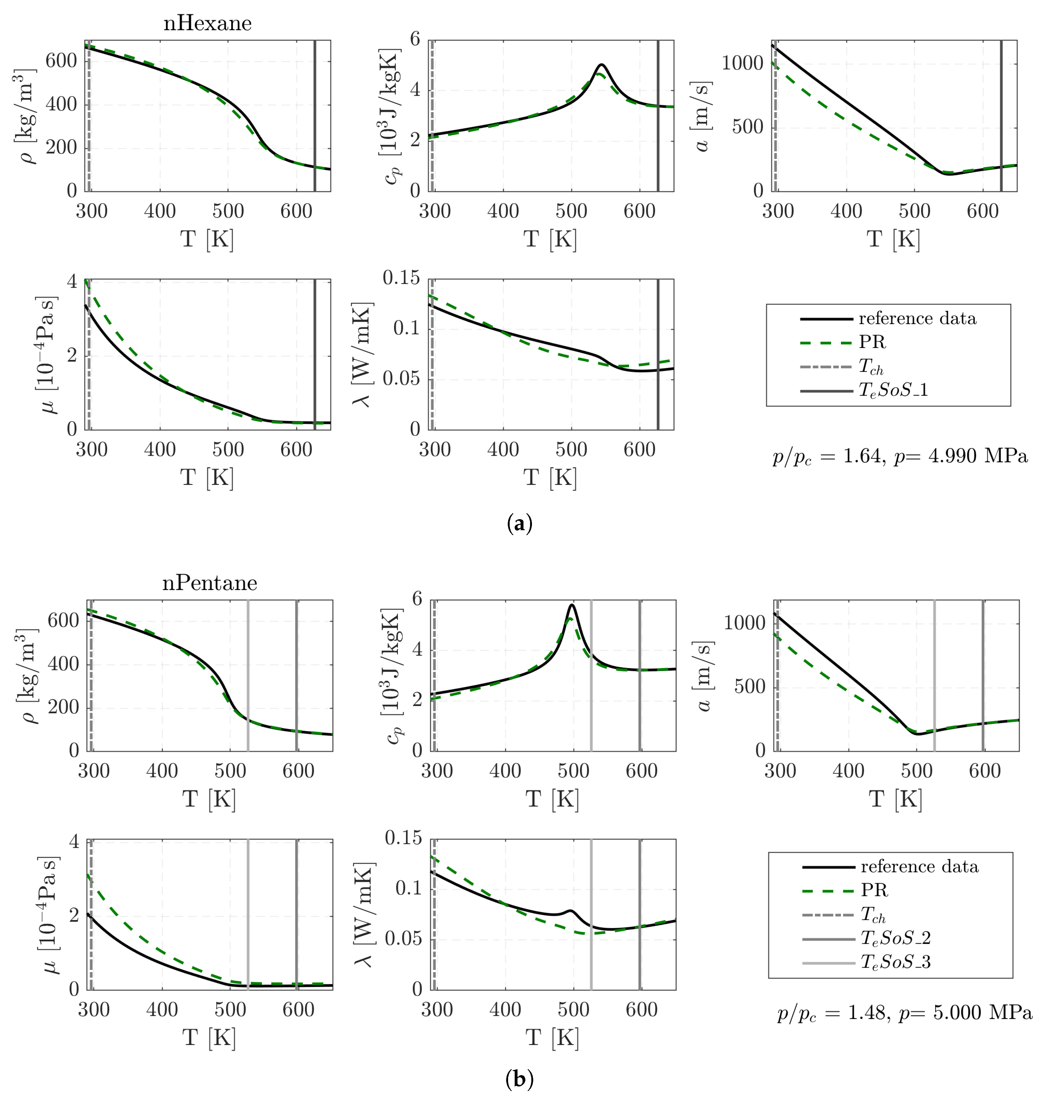
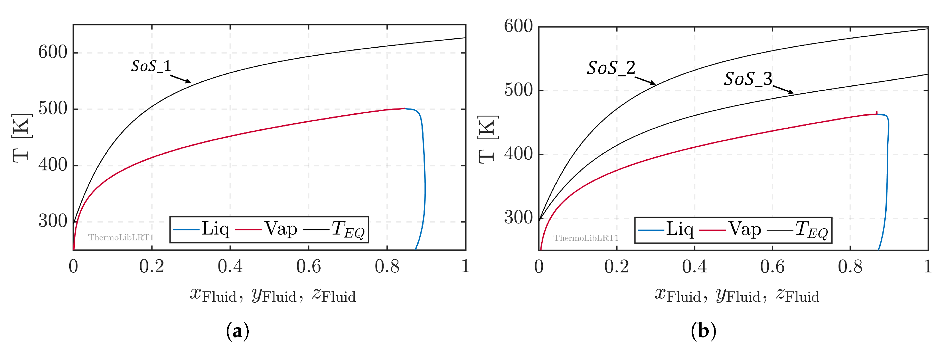
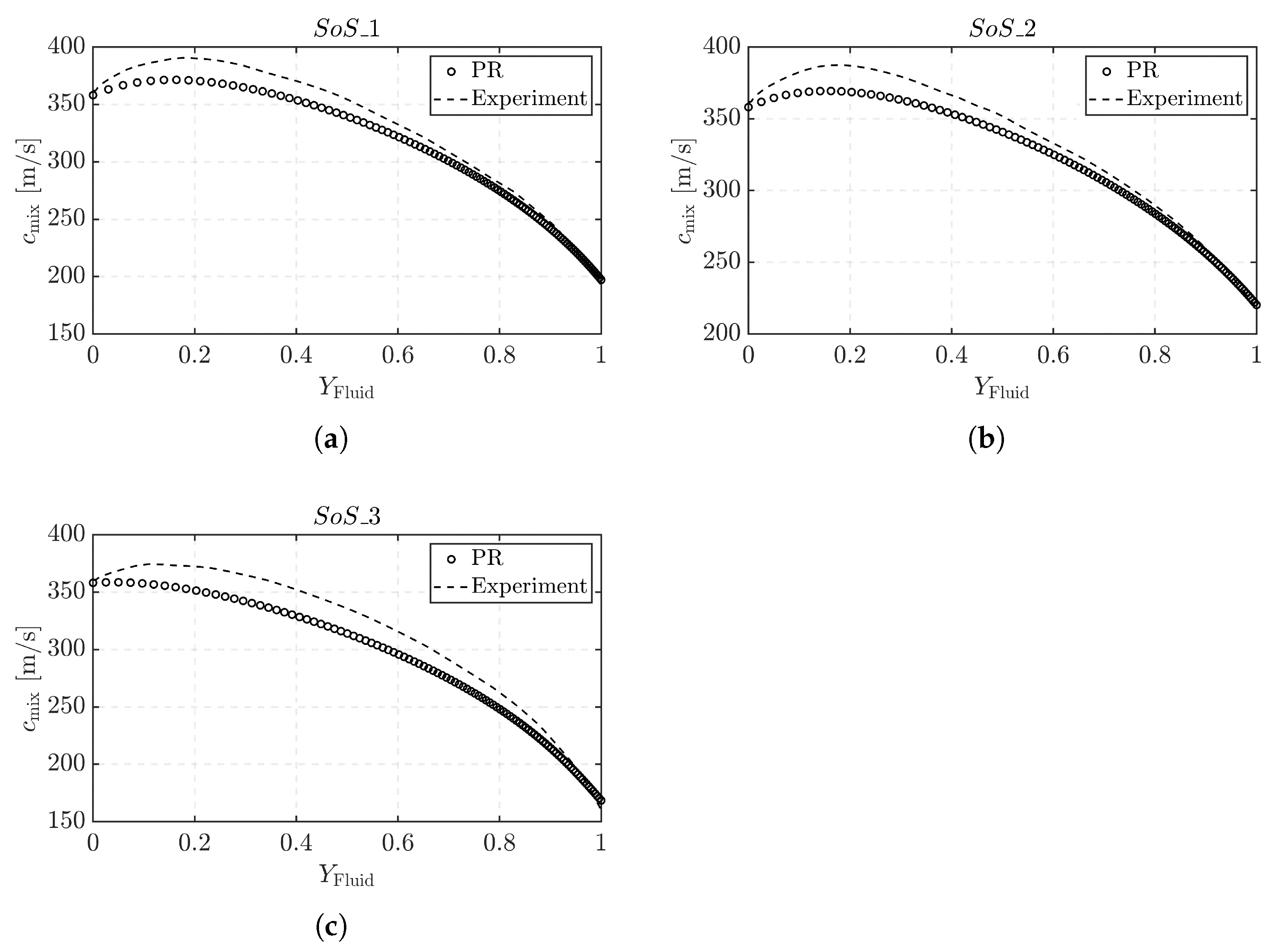
4.1. Thermodynamic Modeling

As a first step, we assess the accuracy of the thermodynamic modeling of the injected fluids at injection conditions (nozzle exit). Afterward, we study the temperature composition diagrams of the considered configurations. Finally, we evaluate the mixture speed of sound as a function of the molar composition and compare the data with the experimental reference data.

Figure 3 compares the thermodynamic modeling of each component—hexane (case SoS_1) and pentane (cases SoS_2 and SoS_3)—at chamber pressure $p=5\mathrm{MPa}$ ($p=4.99\mathrm{MPa}$ for SoS_1) as a function of the temperature. The reference data are obtained from Coolprop [73] and correspond to the Helmholtz EoS. Overall, the thermodynamic model based on the Peng–Robinson cubic EoS reproduces the non-linear behavior of the physical quantities well. Especially for the higher temperatures, which correspond to the injection conditions, a good agreement can be observed. For more details on the modeling accuracy of hexane and pentane using the Peng–Robinson cubic EoS, we refer to Kim et al. [58] and Trummler et al. [56].

In all considered cases, a hot fluid ($T_e=526-627\mathrm{K}$) is injected into nitrogen at room temperature. Consequently, the injected hot fluid is at a gas-like supercritical state at the inlet, see Figure 3. Assuming adiabatic mixing between the injected fluid and the nitrogen in the chamber, temperature composition diagrams can be generated, which are shown in Figure 4. Therein, the mixing temperature is plotted against the molar fraction of the injected fluid. The left end ($x_{Fluid},y_{Fluid},z_{Fluid}=0$) corresponds to pure nitrogen at chamber temperature ($T_{ch}=296\mathrm{K}$) and the right end ($x_{Fluid},y_{Fluid},z_{Fluid}=1$) to the pure injected fluid at injection temperature (see Table 1). Here, x, y, and z refer to the liquid phase composition on a molar basis, the vapor phase composition on a molar basis, and the overall mole fraction. Thus, the path of the adiabatic mixing temperature, which starts at the nozzle outlet and ends somewhere in the chamber in the far field of the jet, would be from right to left in the temperature composition diagram. Additionally, the two-phase region, limited by the bubble-point line (blue) and dew-point line (red), is indicated in Figure 4. The considered cases were designed to study single-phase jet mixing. For this reason, the injection temperature has been chosen high enough to avoid re-condensation due to cooling of the injected fluid, in other words, to avoid crossing the two-phase region in Figure 4.

Figure 5 plots the mixture speed of sound over the mass fraction of the injected fluid. The figure compares the mixture speed of sound obtained with our modeling approach with the experimentally reported data. The mixture speed of sound depends on several quantities (see Equation (24)) and is affected by the temperature (see also single-component effect visible in Figure 3) and the molar composition altering the mixture quantities. In all cases, the mixture speed of sound decreases from pure nitrogen ($Y_{Fluid}=0$) to the pure injected fluid ($Y_{Fluid}=1$). Additionally, it can be seen that the mixture speed of sound describes a parabolic profile peaking at a mass fraction of about $Y_{Fluid}\approx 0.2$. The comparison with the experimental reference data demonstrates that the thermodynamic modeling cannot capture the peak and underestimates the mixture speed of sound at this position by about 5%.

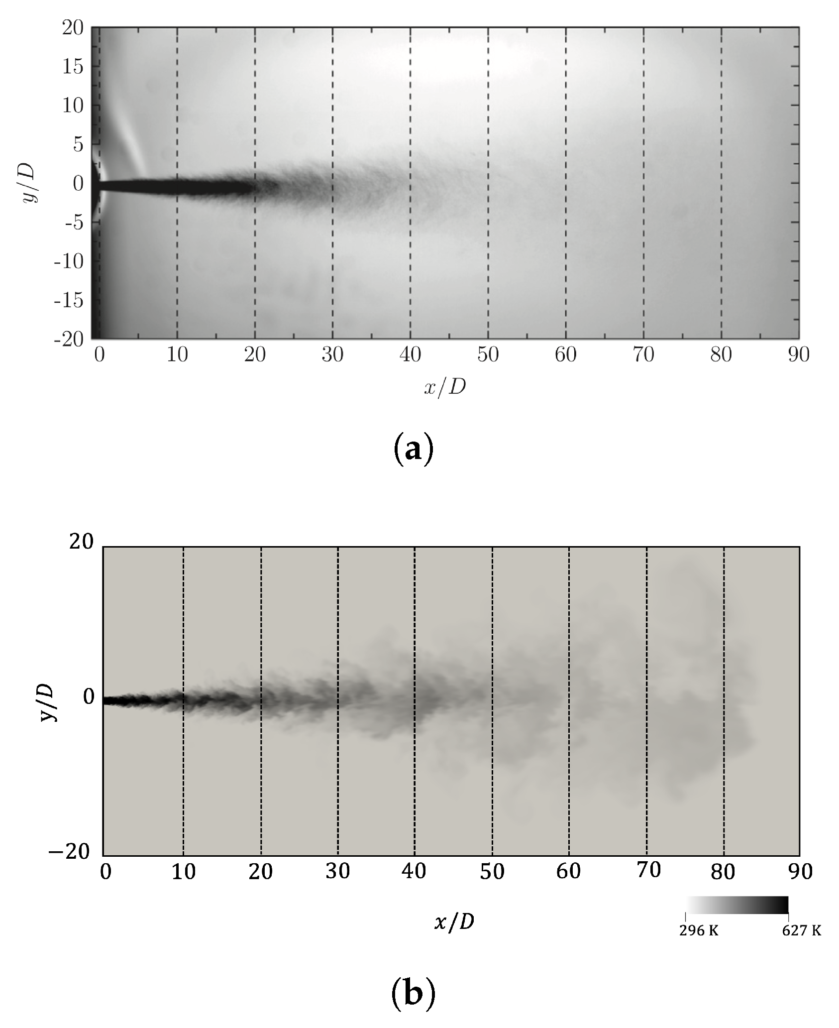
4.2. Single-Phase Jet Mixing

Figure 6 compares an experimental shadowgram of a hexane injection with an instantaneous snapshot of our LES study of $SoS$_1. The compared configurations are not identical, since the experimental work [10] does not contain a visualization of one of the considered cases and only provides a shadowgram of a comparable configuration with $T_e=600\mathrm{K}$ instead of $T_e=627\mathrm{K}$. For the LES results, the temperature field on the midplane is depicted. The temperature distribution is associated with the jet mixing and for this reason often used in the analysis of numerical simulation results [12,14,15]. As discussed in Section 4.1, no phase separation takes place in the considered configurations. Moreover, the considered mixing process is dominated by both turbulence and diffusion effects. As a result, finger-like structures are formed at the periphery of the jet, and the jet gradually dissolves into the environment, as can be seen in the experimental visualization in Figure 6a. Similar structures are visible in the jet periphery of the LES results. Furthermore, the global jet characteristics of the experimental data and our simulations agree well. There is a comparable jet opening, and both figures depict a dense jet core up to $x/D=20$.

The mixing of such configurations is often approximated by adiabatic mixing; see, for example, corresponding temperature composition diagrams in the experimental work [10]. The suitability and applicability of the adiabatic mixing model depends on the relative importance of the local diffusion fluxes and therefore also on the configuration-dependent time and length scales. Baab et al. [78] and Förster et al. [79] showed that the mixing of under-expanded jets can be described well by adiabatic mixing. The high injection velocities at these conditions, together with the eruptive discharge of the fluid, allow for the assumption that heat and mass diffusion are not the dominant effects in the mixing process. For subsonic dense jets, Föll et al. [48] conducted an extended analysis of the binary jet mixing and examined the experimental data [10] considered in the present work. To this end, they evaluated the applicability of the similarity law of Chen and Rodi [80], describing the axial concentration decay for momentum controlled mixing. In Figure 7 the comparison from Föll et al. [48] is reprinted. Contrary to the data of the under-expanded jets [78], not all cases are well described by the similarity law (see Figure 7 and Ref. [48]). While the experimental data of SoS_1 match well with the similarity law and only show minor deviation close to the nozzle exit, the experimental data of SoS_2 and SoS_3 have a higher concentration of the injected fluid in the region after approximately $x/D>20$, where for SoS_3 the deviation is even more pronounced. The higher concentration at the axial position in the experiments implies that the adiabatic mixing overestimates the mixing compared to the experiment. SoS_3 has a lower injection temperature and lower exit velocity than the other two cases (see Table 1), which affects the temperature gradient and the time scale compared to the other two cases. Föll et al. [48] conjectured that the Dufour effect, which refers to a heat flux due to a concentration gradient, might be related with the observations for this case. However, based on LES studies incorporating the Dufour contributions, they could not clarify the influence of the Dufour effect on the jet mixing process due to a presumably too large influence of numerical diffusion.

For LES studies of high temperature and/or high pressure configurations, not only the numerical diffusion itself plays a role, but also whether a fully- or a quasi-conservative formulation of the governing equations is used [15,81]. Ma et al. [81] showed that adiabatic and isochoric mixing are respective limits of the fully- and quasi-conservative formulation, where previous comparative numerical studies of high pressure injections [15,48] found that the experimental data are more accurately predicted by the adiabatic mixing assumption.

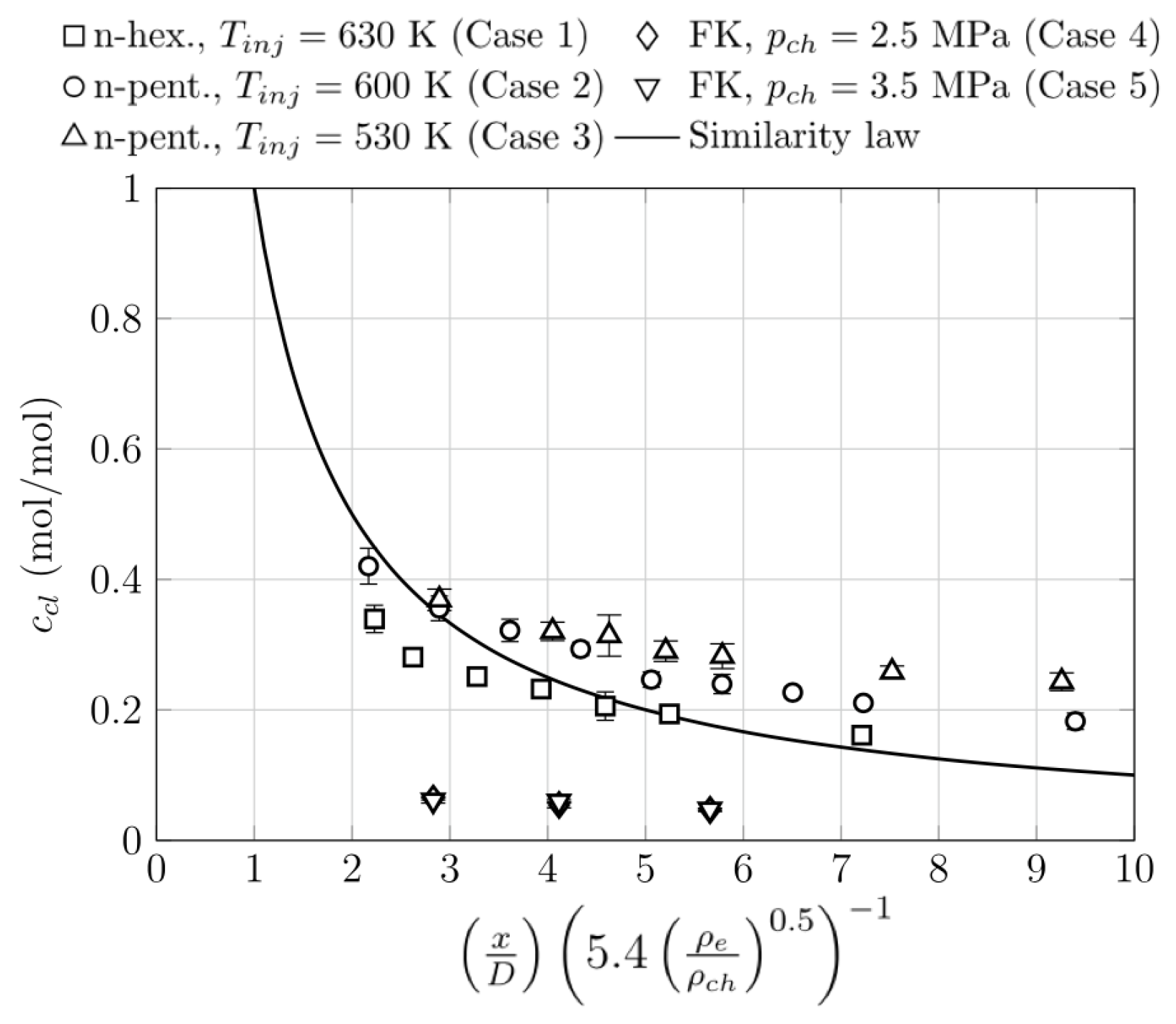
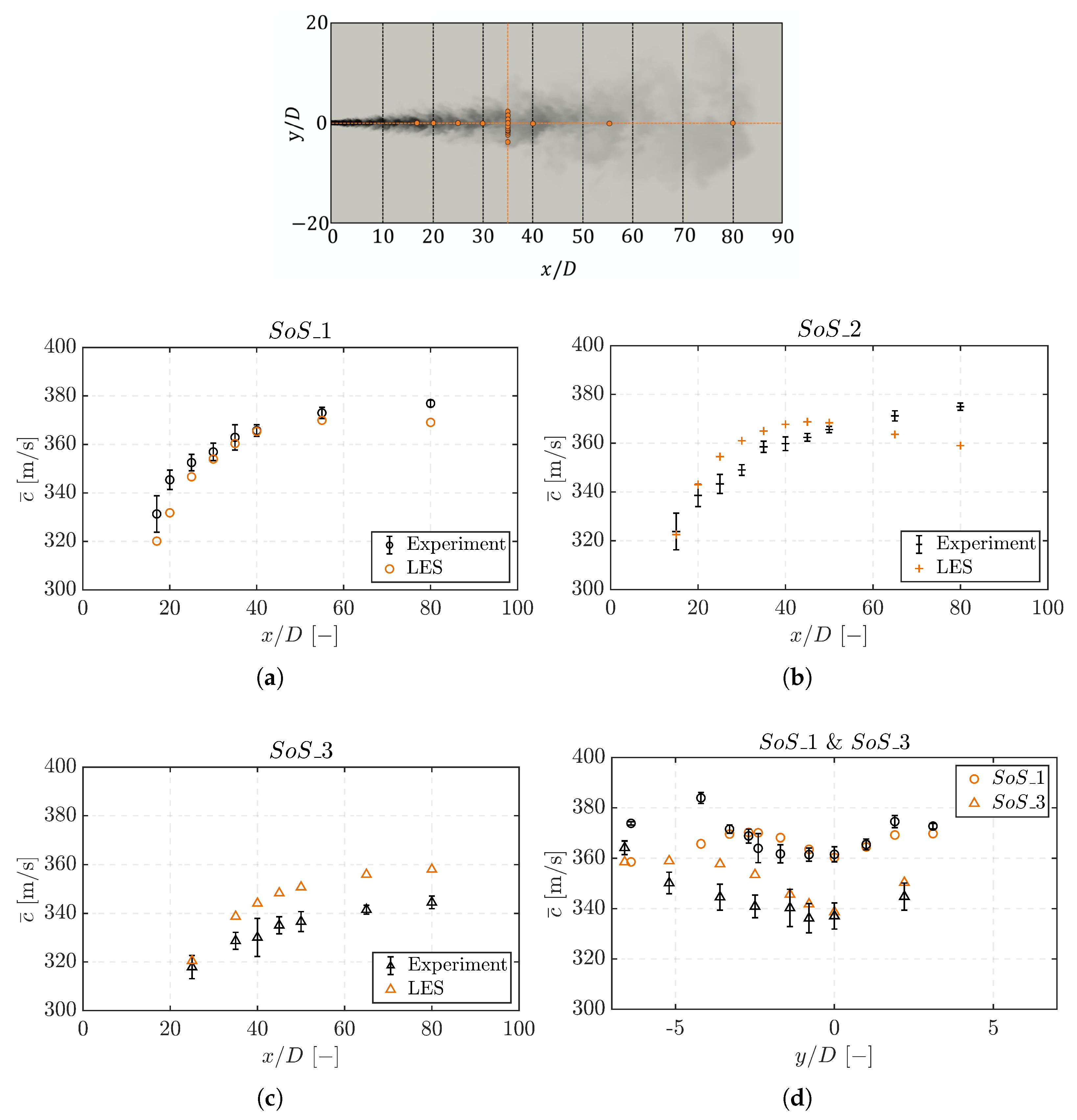
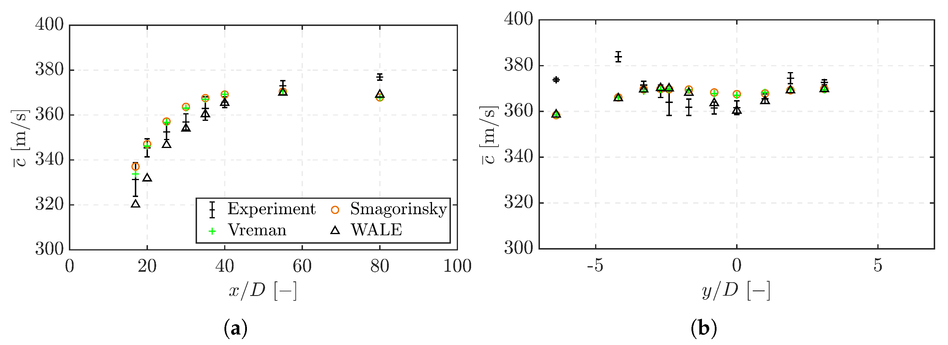
4.3. Validation with Experimental Data

In the experiment, Baab et al. [10] measured the mixture speed of sound at specific axial and radial positions. Figure 8 (top panel) visualizes the measurement positions marked on instantaneous LES results. Figure 8 (main panel) compares the mixture speed of sound obtained in the LES with the experimentally measured ones. The error bars in the experimental data represent the double standard error of the sample mean [10]. Overall, a good qualitative agreement for all three cases can be observed. In the axial direction (Figure 8a–c), the mixture speed of sound gradually increases and asymptotically approaches the value of pure nitrogen with increasing downstream position. The simulation results for SoS_1 tend to slightly underestimate the mixture speed of sound, while these of SoS_2 and SoS_3 tend to overestimate it. In addition to this, SoS_1 and SoS_2 indicate an underestimation at the very downstream positions, where numerical effects, such as a coarser grid, may already have an impact.

In the radial direction (Figure 8d), the mixture speed of sound is increased at the jet periphery due to the higher nitrogen content in this region. Here, only SoS_1 and SoS_3 are compared with the experimental data, since only for these two cases data have been provided. In general, the characteristic curve of the mixture speed of sound is well captured by the LES. In the experimental data, an asymmetry of the profiles is present, which might be associated with the nozzle geometry.

Based on these comparisons, we conclude that the LES qualitatively represents the mixing well under the considered conditions, although the quantitative comparison shows some deviations. We conjecture that besides the differences in experimental and numerical setup (nozzle geometry, boundary conditions, etc.) and numerical effects (grid resolution, numerical scheme, etc.), the fact that adiabatic mixing is not applicable to all the cases of the considered configuration (see above) plays a key role. The simulation results of SoS_2 and SoS_3 tend to overestimate the speed of sound, with the overestimation being more pronounced for SoS_3. Applying these observations to the mixing means that SoS_2 and SoS_3 tend to overestimate it, which is in excellent agreement with the observations by Föll et al. [48].

4.4. Effect of the Sub-Grid Scale Model

In order to assess the effect of the sub-grid scale modeling, additional LES studies of case SoS_1 using the Smagorinsky model and the Vreman model were conducted. Figure 9 compares the averaged mixture speed of sound obtained from the different LES studies. All three models reproduce the general mixing behavior well. In the axial direction (Figure 9a), the mixture speed of sound of the results obtained with the Smagorinsky model and the Vreman model is higher than that of the WALE model, indicating a higher nitrogen content and thus more mixing, which can be assumed to be associated with the more dissipative character of these models. The difference between the models is more pronounced close to the nozzle outlet and vanishes further downstream.

In the radial direction (Figure 9b), the characteristic increase of the mixture speed of sound in the jet mixing region is captured well by all three models and peaks at the same radial position. Regarding the mixture speed of sound in the center region, again, the more dissipative character of Smagorinsky and Vreman compared to WALE is visible. At this axial position ($x/D=35$, center), the WALE model matches the experimental values better than the other two models.

For a comparison of the effects of different LES models in transcritical injections at high pressure, we also refer to previous investigations (e.g., [16,26,29,30]). Müller et al. [26] quantitatively compared and studied results of trans- and supercritical nitrogen injections [4] obtained with the explicit eddy-viscosity models of Smagorinsky and Vreman and the implicit LES approach Adaptive Local Deconvolution Method (ALDM) [82,83]. They found that the sub-grid scale model is less important for the distribution of the averaged quantities than, for example, the inflow conditions (the inflow temperature plays a decisive role in the configuration considered in their study) or the thermodynamic modeling. Jafari et al. [27] presented a qualitative comparison of the results of a transcritical injection with phase transition [14] of the Smagorinsky and the structural Sigma model [84] and observed a shift of the position of the jet break up further upstream and a better agreement with experimental jet opening angle using the Sigma model. Furthermore, for transcritical simulations with phase transition of ECN Spray A, the suitability of the WALE model [25] and the implicit ALDM [13,17,39,43] have been recently demonstrated, where liquid and vapor penetration lengths have been qualitatively compared with experimental data. Furthermore, Lagarza-Cortés et al. [36] obtained good results for LES studies of the Mayer jets [4] using the selective structures-function model by David [85] (see also [86]). For transcritical simulations with phase transition of ECN Spray A, the suitability of the WALE model [25] and the implicit ALDM [13,17,39,43] have been recently demonstrated, where liquid and vapor penetration lengths have been qualitatively compared with experimental data.

Further investigations of the impact of the sub-grid scale modeling in this configuration are the subject of ongoing research at our institute. Due to the strong correlation of the mixture speed of sound with the local molar composition, we consider the LES comparisons of this case to be a valuable extension of previous studies.

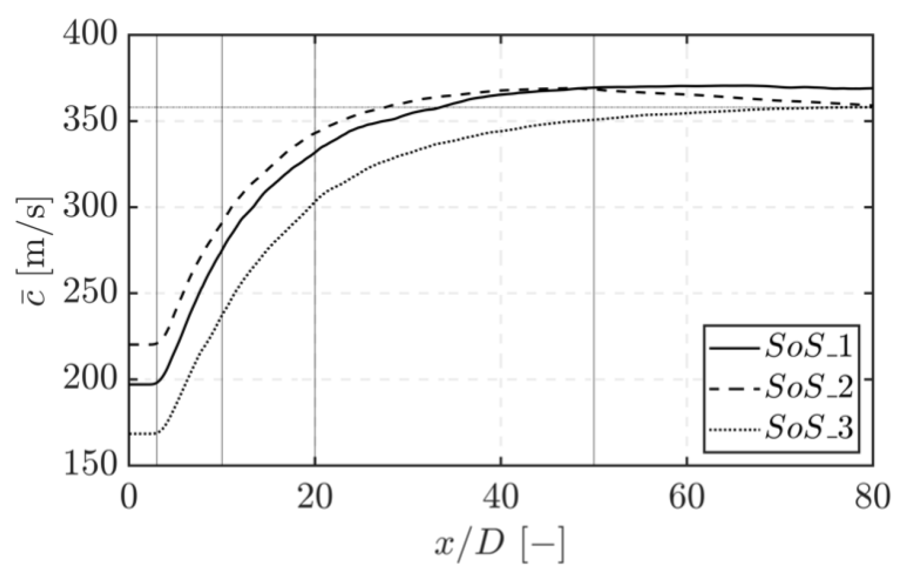
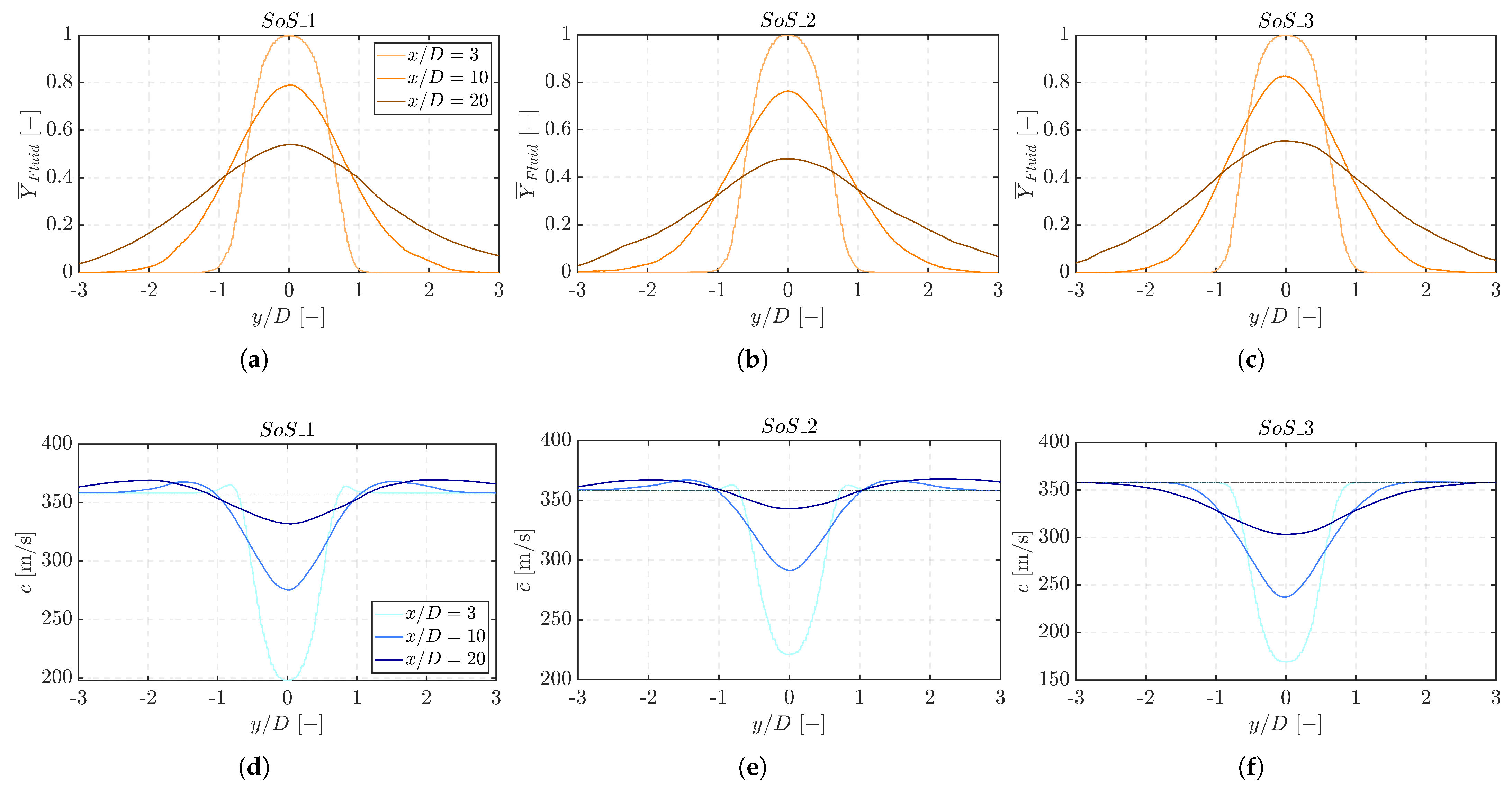
4.5. Detailed Analysis of LES Results

The LES data (WALE model) allow for more detailed analysis and provide a comprehensive database. In the following, we examine the time-averaged data of the mixture speed of sound and the mass fraction distribution in more detail.

Figure 10 compares the mixture speed of sound in the axial direction for the three investigated cases. Due to the different speed of sound values at the injection conditions, the mixture speed of sound starts at different positions at the nozzle outlet ($x/D=0$) and stays at this value until $x/D\approx 3$. This corresponds to the central stream core of the injected fluid (mass fraction $Y_{Fluid}\approx 1$) and is usually very clearly pronounced in CFD simulations [16,20], as described and discussed in detail by Banuti and Hannemann [44]. Due to the similar Reynolds numbers, the length is approximately the same for all three cases. Then, the mixture speed of sound slowly increases downstream due to an increasing nitrogen content, approaching the speed of sound of pure nitrogen. For the cases $SoS$_1 and $SoS$_2, the mixture speed of sound overshoots that of pure nitrogen due to the characteristic curve of the mixture speed of sound, see Figure 5.

Figure 11 depicts the radial profiles of the mass fraction of the injected fluid (Figure 11a–c) together with the mixture speed of sound (Figure 11d–f) at the positions $x/D=\{3,10,20\}$. Again, we see this characteristic increase of the mixture speed of sound at the jet periphery, which results in an overshoot at this position in $SoS$_1 and $SoS$_2 (see Figure 11d,e). At $SoS$_3 (Figure 11f), no overshoot is visible, which is correlated with the modeled mixture speed of sound, see Figure 5c.

The data provided here containing both the mixture speed of sound and the mass fraction for three different high pressure injections can serve as a benchmark for future numerical investigations in this field. The availability of both data sets allows for easier identification of reasons for deviations and discrepancies.

5. Conclusions and Outlook

We have presented the thermodynamic modeling and LES simulation results of multi-component jet mixing at high pressure conditions. The employed thermodynamic model is based on a cubic EoS for multi-component flows and combined with the Chung correlations for modeling the transport properties. The LES studies were conducted using an extended version of the open-source code OpenFOAM, including special modifications to account for real gas thermodynamics. Using this framework, we simulated three selected cases from the experimental study by Baab et al. [10]—one hexane injection and two pentane injections that differ in injection temperature and injection velocity.

First, we assessed the accuracy of thermodynamic modeling and the characteristics of the mixture speed of sound. With the employed thermodynamic modeling approach, we were able to capture and reproduce the strongly non-linear behavior at the considered pressure and temperature conditions. Moreover, the evaluation of the mixture speed of sound was presented, and its behavior along the adiabatic mixing temperature was analyzed for the three considered cases.

Using the experimental data, we were able to validate our numerical approach and demonstrate the suitability of LES studies for mixing processes. The LES results show the same characteristic trends observed in the experiments. The quantitative comparison revealed certain deviations that seem to be associated with the fact that adiabatic mixing is not globally applicable to the considered configurations. The observed deviations can be well explained with recent analyses in the literature.

In addition to this, we compared simulation results obtained using the Smagorinsky, the Vreman, and the WALE sub-grid scale model. All three models can capture the characteristic mixing, but the less dissipative WALE model showed the best agreement with the experimentally measured radial distribution of the mixture speed of sound. More thorough investigations are necessary and part of current research.

Finally, detailed data from the LES study were presented and discussed. For this purpose, data on the mixture speed of sound and the corresponding mass fraction were extracted at selected radial positions of the jet.

The main findings can be summarized as: (i) the mixture speed of sound is well-suited to quantitatively investigate mixing processes in experimental as well as numerical studies; (ii) single-phase jet mixing can be well represented by LES investigations; (iii) all three applied sub-grid scale models (Smagorinsky, Vreman, and WALE) can capture the characteristic mixing.

The present work extends the previous numerical studies on this subject presenting an LES study of three cases, which were experimentally documented, and closely examining the thermodynamics and the correlation of multi-component mixing and the mixture speed of sound. Nevertheless, further validations and investigations in this field are required. Unfortunately, due to the limited data on fluoroketone and the limitations of the thermodynamic model used, studies on the other two configurations of the experiment cannot be performed. To further validate our modeling approach and shed more light on the underlying physics, joint experimental and numerical studies of multi-component jet mixing are planned [87]. Based on the complementary insights from numerical flow simulations and experiments, a more comprehensive understanding of the underlying physical mechanisms and phenomena may be gained.

References

1. Anitescu, G.; Tavlarides, L.L.; Geana, D. Phase transitions and thermal behavior of fuel- diluent mixtures. Energy Fuels 2009, 23, 3068–3077. [Google Scholar] [CrossRef]
2. De Boer, C.; Bonar, G.; Sasaki, S.; Shetty, S. Application of Supercritical Gasoline Injection to a Direct Injection Spark Ignition Engine for Particulate Reduction; Technical Report No. 2013-01-0257, SAE Technical Paper; SAE: Warrendale, PA, USA, 2013. [Google Scholar]
3. Chehroudi, B. Recent experimental efforts on high-pressure supercritical injection for liquid rockets and their implications. Int. J. Aerosp. Eng. 2012, 2012, 121802. [Google Scholar] [CrossRef] [Green Version]
4. Mayer, W.; Telaar, J.; Branam, R.; Schneider, G.; Hussong, J. Raman measurements of cryogenic injection at supercritical pressure. Heat Mass Transf. 2003, 39, 709–719. [Google Scholar] [CrossRef]
5. Oschwald, M.; Smith, J.; Branam, R.; Hussong, J.; Schik, A.; Chehroudi, B.; Talley, D. Injection of fluids into supercritical environments. Combust. Sci. Technol. 2006, 178, 49–100. [Google Scholar] [CrossRef]
6. Klima, T.C.; Peter, A.; Riess, S.; Wensing, M.; Braeuer, A.S. Quantification of mixture composition, liquid-phase fraction and-temperature in transcritical sprays. J. Supercrit. Fluids 2020, 159, 104777. [Google Scholar] [CrossRef]
7. Roy, A.; Segal, C. Experimental study of fluid jet mixing at supercritical conditions. J. Propuls. Power 2010, 26, 1205–1211. [Google Scholar] [CrossRef]
8. Roy, A.; Joly, C.; Segal, C. Disintegrating supercritical jets in a subcritical environment. J. Fluid Mech. 2013, 717, 193–202. [Google Scholar] [CrossRef]
9. Steinhausen, C.; Gerber, V.; Preusche, A.; Weigand, B.; Dreizler, A.; Lamanna, G. On the potential and challenges of laser-induced thermal acoustics for experimental investigation of macroscopic fluid phenomena. Exp. Fluids 2021, 62, 1–16. [Google Scholar] [CrossRef]
10. Baab, S.; Steinhausen, C.; Lamanna, G.; Weigand, B.; Förster, F. A quantitative speed of sound database for multi-component jet mixing at high pressure. Fuel 2018, 233, 918–925. [Google Scholar] [CrossRef]
11. Qiu, L.; Reitz, R.D. Simulation of supercritical fuel injection with condensation. Int. J. Heat Mass Transf. 2014, 79, 1070–1086. [Google Scholar] [CrossRef] [Green Version]
12. Traxinger, C. Real-Gas Effects and Single-Phase Instabilities during Injection, Mixing and Combustion under High-Pressure Conditions. Ph.D. Thesis, Bundeswehr University Munich, Munich, Germany, 2021. [Google Scholar]
13. Fathi, M.; Hickel, S.; Roekaerts, D. Large eddy simulations of reacting and non-reacting transcritical fuel sprays using multiphase thermodynamics. Phys. Fluids 2022, 34, 085131. [Google Scholar] [CrossRef]
14. Traxinger, C.; Mueller, H.; Pfitzner, M.; Baab, S.; Lamanna, G.; Weigand, B.; Matheis, J.; Stemmer, C.; Adams, N.A.; Hickel, S. Experimental and numerical investigation of phase separation due to multicomponent mixing at high-pressure conditions. In Proceedings of the 28th Conference on Liquid Atomization and Spray System, Chicago, IL, USA, 22–26 July 2018. [Google Scholar]
15. Matheis, J.; Hickel, S. Multi-component vapor-liquid equilibrium model for LES of high-pressure fuel injection and application to ECN Spray A. Int. J. Multiph. Flow 2018, 99, 294–311. [Google Scholar] [CrossRef]
16. Müller, H.; Pfitzner, M.; Matheis, J.; Hickel, S. Large-eddy simulation of coaxial LN2/GH2 injection at trans-and supercritical conditions. J. Propuls. Power 2016, 32, 46–56. [Google Scholar] [CrossRef]
17. Matheis, J.; Müller, H.; Lenz, C.; Pfitzner, M.; Hickel, S. Volume translation methods for real-gas computational fluid dynamics simulations. J. Supercrit. Fluids 2016, 107, 422–432. [Google Scholar] [CrossRef]
18. Lapenna, P.E.; Creta, F. Mixing under transcritical conditions: An a-priori study using direct numerical simulation. J. Supercrit. Fluids 2017, 128, 263–278. [Google Scholar] [CrossRef]
19. Lapenna, P.; Creta, F. Direct numerical simulation of transcritical jets at moderate reynolds number. AIAA J. 2019, 57, 2254–2263. [Google Scholar] [CrossRef]
20. Sharan, N.; Bellan, J. Investigation of high-pressure turbulent jets using direct numerical simulation. J. Fluid Mech. 2021, 922, A24. [Google Scholar] [CrossRef]
21. Sou, A.; Hosokawa, S.; Tomiyama, A. Effects of cavitation in a nozzle on liquid jet atomization. Int. J. Heat Mass Transf. 2007, 50, 3575–3582. [Google Scholar] [CrossRef] [Green Version]
22. Sou, A.; Biçer, B.; Tomiyama, A. Numerical simulation of incipient cavitation flow in a nozzle of fuel injector. Comput. Fluids 2014, 103, 42–48. [Google Scholar] [CrossRef]
23. Örley, F.; Trummler, T.; Hickel, S.; Mihatsch, M.; Schmidt, S.; Adams, N. Large-eddy simulation of cavitating nozzle flow and primary jet break-up. Phys. Fluids 2015, 27, 086101. [Google Scholar] [CrossRef] [Green Version]
24. Trummler, T.; Rahn, D.; Schmidt, S.J.; Adams, N.A. Large eddy simulations of cavitating flow in a step nozzle with injection into gas. At. Sprays 2018, 28, 931–955. [Google Scholar] [CrossRef]
25. Koukouvinis, P.; Vidal-Roncero, A.; Rodriguez, C.; Gavaises, M.; Pickett, L. High pressure/high temperature multiphase simulations of dodecane injection to nitrogen: Application on ECN Spray-A. Fuel 2020, 275, 117871. [Google Scholar] [CrossRef]
26. Müller, H.; Niedermeier, C.A.; Matheis, J.; Pfitzner, M.; Hickel, S. Large-eddy simulation of nitrogen injection at trans- and supercritical conditions. Phys. Fluids 2016, 28, 015102. [Google Scholar] [CrossRef]
27. Jafari, S.; Gaballa, H.; Habchi, C.; De Hemptinne, J.C.; Mougin, P. Exploring the interaction between phase separation and turbulent fluid dynamics in multi-species supercritical jets using a tabulated real-fluid model. J. Supercrit. Fluids 2022, 184, 105557. [Google Scholar] [CrossRef]
28. Klein, M.; Sadiki, A.; Janicka, J. A digital filter based generation of inflow data for spatially developing direct numerical or large eddy simulations. J. Comput. Phys. 2003, 186, 652–665. [Google Scholar] [CrossRef]
29. Selle, L.C.; Okong’o, N.A.; Bellan, J.; Harstad, K.G. Modelling of subgrid-scale phenomena in supercritical transitional mixing layers: An a priori study. J. Fluid Mech. 2007, 593, 57–91. [Google Scholar] [CrossRef] [Green Version]
30. Petit, X.; Ribert, G.; Lartigue, G.; Domingo, P. Large-eddy simulation of supercritical fluid injection. J. Supercrit. Fluids 2013, 84, 61–73. [Google Scholar] [CrossRef]
31. Haidn, O.; Habiballah, M. Research on high pressure cryogenic combustion. Aerosp. Sci. Technol. 2003, 7, 473–491. [Google Scholar] [CrossRef]
32. Habiballah, M.; Orain, M.; Grisch, F.; Vingert, L.; Gicquel, P. Experimental studies of high-pressure cryogenic flames on the Mascotte facility. Combust. Sci. Technol. 2006, 178, 101–128. [Google Scholar] [CrossRef]
33. Zong, N.; Meng, H.; Hsieh, S.Y.; Yang, V. A numerical study of cryogenic fluid injection and mixing under supercritical conditions. Phys. Fluids 2004, 16, 4248–4261. [Google Scholar] [CrossRef] [Green Version]
34. Kim, T.; Kim, Y.; Kim, S.K. Numerical study of cryogenic liquid nitrogen jets at supercritical pressures. J. Supercrit. Fluids 2011, 56, 152–163. [Google Scholar] [CrossRef]
35. Park, T.S. LES and RANS simulations of cryogenic liquid nitrogen jets. J. Supercrit. Fluids 2012, 72, 232–247. [Google Scholar] [CrossRef]
36. Lagarza-Cortés, C.; Ramírez-Cruz, J.; Salinas-Vázquez, M.; Vicente-Rodríguez, W.; Cubos-Ramírez, J.M. Large-eddy simulation of transcritical and supercritical jets immersed in a quiescent environment. Phys. Fluids 2019, 31, 025104. [Google Scholar] [CrossRef]
37. Poblador-Ibanez, J.; Sirignano, W.A. A volume-of-fluid method for variable-density, two-phase flows at supercritical pressure. Phys. Fluids 2022, 34, 053321. [Google Scholar] [CrossRef]
38. Chung, T.H.; Ajlan, M.; Lee, L.L.; Starling, K.E. Generalized multiparameter correlation for nonpolar and polar fluid transport properties. Ind. Eng. Chem. Res. 1988, 27, 671–679. [Google Scholar] [CrossRef]
39. Matheis, J. Numerical Simulation of Fuel Injection and Turbulent Mixing Under High-Pressure Conditions. Ph.D. Thesis, Technical University Munich, Munich, Germany, 2018. [Google Scholar]
40. Doehring, A.; Kaller, T.; Schmidt, S.J.; Adams, N.A. Large-eddy simulation of turbulent channel flow at transcritical states. Int. J. Heat Fluid Flow 2021, 89, 108781. [Google Scholar] [CrossRef]
41. Reid, R.C.; Prausnitz, J.M.; Poling, B.E. The Properties of Gases and Liquids; McGraw Hill Book Co.: New York, NY, USA, 1987. [Google Scholar]
42. Miller, R.S.; Harstad, K.G.; Bellan, J. Direct numerical simulations of supercritical fluid mixing layers applied to heptane–nitrogen. J. Fluid Mech. 2001, 436, 1–39. [Google Scholar] [CrossRef] [Green Version]
43. Matheis, J.; Hickel, S. Multi-component vapor-liquid equilibrium model for LES and application to ECN Spray A. In Proceedings Stanford Summer School; Center for Turbulence Research: Stanford, CA, USA, 2016. [Google Scholar]
44. Banuti, D.T.; Hannemann, K. The absence of a dense potential core in supercritical injection: A thermal break-up mechanism. Phys. Fluids 2016, 28, 035103. [Google Scholar] [CrossRef]
45. Terashima, H.; Koshi, M. Unique characteristics of cryogenic nitrogen jets under supercritical pressures. J. Propuls. Power 2013, 29, 1328–1336. [Google Scholar] [CrossRef]
46. Schmitt, T.; Selle, L.; Ruiz, A.; Cuenot, B. Large-eddy simulation of supercritical-pressure round jets. AIAA J. 2010, 48, 2133–2144. [Google Scholar] [CrossRef]
47. Jafari, S.; Gaballa, H.; Habchi, C.; de Hemptinne, J.C. Towards Understanding the Structure of Subcritical and Transcritical Liquid–Gas Interfaces Using a Tabulated Real Fluid Modeling Approach. Energies 2021, 14, 5621. [Google Scholar] [CrossRef]
48. Föll, F.; Gerber, V.; Munz, C.D.; Weigand, B.; Lamanna, G. On the consideration of diffusive fluxes within high-pressure injections. In Future Space-Transport-System Components under High Thermal and Mechanical Loads; Springer: Cham, Switzerland, 2021; pp. 195–208. [Google Scholar]
49. Smagorinsky, J. General circulation model of the atmosphere. Mon. Weather Rev. 1963, 91, 99–164. [Google Scholar] [CrossRef]
50. Vreman, A. An eddy-viscosity subgrid-scale model for turbulent shear flow: Algebraic theory and applications. Phys. Fluids 2004, 16, 3670–3681. [Google Scholar] [CrossRef]
51. Ducros, F.; Nicoud, F.; Poinsot, T. Wall-adapting local eddy-viscosity models for simulations in complex geometries. In Numerical Methods for Fluid Dynamics VI; ICFD: Oxford, UK, 1998; pp. 293–299. [Google Scholar]
52. Prosperetti, A.; Tryggvason, G. Computational Methods for Multiphase Flow; Cambridge University Press: Cambridge, UK, 2007. [Google Scholar]
53. Zips, J.; Traxinger, C.; Pfitzner, M. Time-resolved flow field and thermal loads in a single-element GOx/GCH4 rocket combustor. Int. J. Heat Mass Transf. 2019, 143, 118474. [Google Scholar] [CrossRef]
54. Yao, M.X.; Hickey, J.P.; Ma, P.C.; Ihme, M. Molecular diffusion and phase stability in high-pressure combustion. Combust. Flame 2019, 210, 302–314. [Google Scholar] [CrossRef]
55. Peng, D.Y.; Robinson, D.B. A new two-constant equation of state. Ind. Eng. Chem. Fundam. 1976, 15, 59–64. [Google Scholar] [CrossRef]
56. Trummler, T.; Glatzle, M.; Doehring, A.; Urban, N.; Klein, M. Thermodynamic modeling for numerical simulations based on the generalized cubic equation of state. Phys. Fluids 2022, 34, 116126. [Google Scholar] [CrossRef]
57. Cismondi, M.; Mollerup, J. Development and application of a three-parameter RK–PR equation of state. Fluid Phase Equilibria 2005, 232, 74–89. [Google Scholar] [CrossRef]
58. Kim, S.K.; Choi, H.S.; Kim, Y. Thermodynamic modeling based on a generalized cubic equation of state for kerosene/LOx rocket combustion. Combust. Flame 2012, 159, 1351–1365. [Google Scholar] [CrossRef]
59. Poling, B.E.; Prausnitz, J.M.; O’Connell, J.P. The Properties of Gases and Liquids; McGraw-Hill: New York, NY, USA, 2001; Volume 5. [Google Scholar]
60. Elliott, J.R.; Lira, C.T. Introductory Chemical Engineering Thermodynamics; Prentice Hall: Upper Saddle River, NJ, USA, 2012; Volume 668. [Google Scholar]
61. Goos, E.; Burcat, A.; Ruscic, B. Third Millennium Ideal Gas and Condensed Phase Thermochemical Database for Combustion; The University of Chicago: Chicago, IL, USA, 2009. [Google Scholar]
62. Issa, R.I. Solution of the implicitly discretised fluid flow equations by operator-splitting. J. Comput. Phys. 1986, 62, 40–65. [Google Scholar] [CrossRef]
63. Issa, R.; Ahmadi-Befrui, B.; Beshay, K.; Gosman, A. Solution of the implicitly discretised reacting flow equations by operator-splitting. J. Comput. Phys. 1991, 93, 388–410. [Google Scholar] [CrossRef]
64. Jarczyk, M.M.; Pfitzner, M. Large eddy simulation of supercritical nitrogen jets. In Proceedings of the 50th AIAA Aerospace Sciences Meeting including the New Horizons Forum and Aerospace Exposition, Nashville, TN, USA, 9–12 January 2012; p. 1270. [Google Scholar]
65. Traxinger, C.; Zips, J.; Banholzer, M.; Pfitzner, M. A pressure-based solution framework for sub-and supersonic flows considering real-gas effects and phase separation under engine-relevant conditions. Comput. Fluids 2020, 202, 104452. [Google Scholar] [CrossRef]
66. Banholzer, M.; Vera-Tudela, W.; Traxinger, C.; Pfitzner, M.; Wright, Y.; Boulouchos, K. Numerical investigation of the flow characteristics of underexpanded methane jets. Phys. Fluids 2019, 31, 056105. [Google Scholar] [CrossRef]
67. Traxinger, C.; Pfitzner, M. Effect of nonideal fluid behavior on the jet mixing process under high-pressure and supersonic flow conditions. J. Supercrit. Fluids 2021, 172, 105195. [Google Scholar] [CrossRef]
68. Müller, H. Simulation turbulenter nicht-vorgemischter Verbrennung bei überkritischen Drücken. Ph.D. Thesis, Bundeswehr University Munich, Munich, Germany, 2016. [Google Scholar]
69. Patankar, S.V.; Spalding, D.B. A calculation procedure for heat, mass and momentum transfer in three-dimensional parabolic flows. In Numerical Prediction of Flow, Heat Transfer, Turbulence and Combustion; Elsevier: Amsterdam, The Netherlands, 1983; pp. 54–73. [Google Scholar]
70. Issa, R.I.; Gosman, A.; Watkins, A. The computation of compressible and incompressible recirculating flows by a non-iterative implicit scheme. J. Comput. Phys. 1986, 62, 66–82. [Google Scholar] [CrossRef]
71. Kaller, T.; Pasquariello, V.; Hickel, S.; Adams, N.A. Turbulent flow through a high aspect ratio cooling duct with asymmetric wall heating. J. Fluid Mech. 2019, 860, 258–299. [Google Scholar] [CrossRef] [Green Version]
72. Koukouvinis, P.; Naseri, H.; Gavaises, M. Performance of turbulence and cavitation models in prediction of incipient and developed cavitation. Int. J. Engine Res. 2017, 18, 333–350. [Google Scholar] [CrossRef]
73. Bell, I.H.; Wronski, J.; Quoilin, S.; Lemort, V. Pure and pseudo-pure fluid thermophysical property evaluation and the open-source thermophysical property library CoolProp. Ind. Eng. Chem. Res. 2014, 53, 2498–2508. [Google Scholar] [CrossRef] [Green Version]
74. Batchelor, G.K. The Theory of Homogeneous Turbulence; Cambridge University Press: Cambridge, UK, 1953. [Google Scholar]
75. Unnikrishnan, U.; Huo, H.; Wang, X.; Yang, V. Subgrid scale modeling considerations for large eddy simulation of supercritical turbulent mixing and combustion. Phys. Fluids 2021, 33, 075112. [Google Scholar] [CrossRef]
76. Immer, M.C. Time-resolved measurement and simulation of local scale turbulent urban flow. Ph.D. Thesis, ETH Zurich, Zurich, Switzerland, 2016. [Google Scholar]
77. Ketterl, S. Large-Eddy Simulation des Primärzerfalls von Flüssigkeitsstrahlen. Ph.D. Thesis, Bundeswehr University Munich, Munich, Germany, 2019. [Google Scholar]
78. Baab, S.; Förster, F.; Lamanna, G.; Weigand, B. Speed of sound measurements and mixing characterization of underexpanded fuel jets with supercritical reservoir condition using laser-induced thermal acoustics. Exp. Fluids 2016, 57, 1–13. [Google Scholar] [CrossRef]
79. Förster, F.J.; Baab, S.; Steinhausen, C.; Lamanna, G.; Ewart, P.; Weigand, B. Mixing characterization of highly underexpanded fluid jets with real gas expansion. Exp. Fluids 2018, 59, 1–10. [Google Scholar] [CrossRef] [Green Version]
80. Chen, C.J.; Rodi, W. Vertical turbulent buoyant jets: A review of experimental data. NASA Sti/Recon Technical Report A 1980, 80, 23073. [Google Scholar]
81. Ma, P.C.; Wu, H.; Banuti, D.T.; Ihme, M. On the numerical behavior of diffuse-interface methods for transcritical real-fluids simulations. Int. J. Multiph. Flow 2019, 113, 231–249. [Google Scholar] [CrossRef]
82. Hickel, S.; Adams, N.A.; Domaradzki, J.A. An adaptive local deconvolution method for implicit LES. J. Comput. Phys. 2006, 213, 413–436. [Google Scholar] [CrossRef]
83. Hickel, S.; Egerer, C.P.; Larsson, J. Subgrid-scale modeling for implicit large eddy simulation of compressible flows and shock-turbulence interaction. Phys. Fluids 2014, 26, 106101. [Google Scholar] [CrossRef]
84. Nicoud, F.; Toda, H.B.; Cabrit, O.; Bose, S.; Lee, J. Using singular values to build a subgrid-scale model for large eddy simulations. Phys. Fluids 2011, 23, 085106. [Google Scholar] [CrossRef] [Green Version]
85. David, E. Modélisation des écoulements compressibles et hypersoniques: Une approche instationnaire. Ph.D. Thesis, Grenoble INPG, Grenoble, France, 1993. [Google Scholar]
86. Lesieur, M.; Metais, O. New trends in large-eddy simulations of turbulence. Annu. Rev. Fluid Mech. 1996, 28, 45–82. [Google Scholar] [CrossRef]
87. Neumann, P.; Das Sharma, A.; Viot, L.; Trummler, T.; Doehring, A.; Son, M.; Auweter, A.; Gross, J.; Stierle, R.; Tippmann, N.; et al. MaST: Scale-Bridging Exploration of Transcritical Fluid Systems; Universitat der Bundeswehr Hamburg: Hamburg, Germany, 2022. [Google Scholar]
Figure 1. (a) Simulation domain; (b) grid on the midplane overlaid to the temperature distribution on the midplane; (c) grid resolution in the nozzle cross section. To promote visibility only every second grid line is shown. Note that there are graphical artifacts from the visualization using ParaView.
Energies 16 02113 g001
Figure 2. Grid convergence study for the mean density extracted along the center line for case SoS_1. Coarse, medium, fine refer to grid resolutions 30, 45, and 60 cells over the nozzle diameter.
Energies 16 02113 g002
Figure 3. Thermodynamic modeling using the Peng–Robinson EoS for nHexane in (a) and for nPentane in (b). Reference data [73] is included for comparison. Figures are generated using realtpl [56].
Energies 16 02113 g003
Figure 4. Temperature composition diagram for hexane/nitrogen ( S o S _1) in (a) and pentane/nitrogen ( S o S _2, S o S _3) in (b). The two-phase region, limited by the bubble-point line (blue) and dew-point line (red), is additionally indicated.
Energies 16 02113 g004
Figure 5. Mixture speed of sound as a function of the mass fraction of the injected fluid ( Y F l u i d ) for S o S _1 (a), S o S _2 (b), S o S _3 (c). “PR” refers to the data obtained with our thermodynamic modeling approach and “Experiment" to the experimental reference data [10].
Energies 16 02113 g005
Figure 6. (a) Exemplary shadowgram of a hexane jet ( T e = 600 K , p c h = 5 MPa , T c h = 293 K ) reprinted from Baab et al. [10] (a shadowgram corresponding to one of the considered cases was not provided in Ref. [10]); (b) instantaneous temperature field on the midplane of case SoS_1 (hexane) ( T e = 627 K , p c h = 4.99 MPa , T c h = 296 K ).
Energies 16 02113 g006
Figure 7. Comparison of the axial mass fraction distribution of the experiment [78] (symbols) with the similarity law of Chen and Rodi [80] (solid line). Case 1, Case 2, and Case 3 correspond to SoS_1, SoS_2, and SoS_3. The figure is reprinted from Föll et al. [48].
Energies 16 02113 g007
Figure 8. Top panel: Experimental measurement positions of the mixture speed of sound indicated on LES results. Main panel: Comparison of the mixture speed of sound of the LES (orange) and the experiment (black) (error bars represent the double standard error of the sample mean) for the cases S o S _ 1 (a), S o S _ 2 (b), and S o S _ 3 (c) in the axial direction and for the cases S o S _ 1 and S o S _ 3 in the radial direction at the position x / D = 35 (d).
Energies 16 02113 g008
Figure 9. Comparison of the mixture speed of sound of LES studies using different sub-grid scale models (color) and the experiment (black) for the cases S o S _ 1 in the axial direction (a) and in the radial direction at the position x / D = 35 (b).
Energies 16 02113 g009
Figure 10. Time-averaged mixture speed of sound along the center line. The horizontal line at c 355 m / s corresponds to the speed of sound of pure nitrogen.
Energies 16 02113 g010
Figure 11. Radial profiles of the mass fraction of the injected fluid (ac) and the mixture speed of sound (df) at the axial positions x / D = { 3 , 10 , 20 } . Data in (a,d) correspond to SoS_1, in (b,e) to SoS_2 and in (e,f) to SoS_3.
Energies 16 02113 g011