New Method of Modeling Daily Energy Consumption

Abstract

At present, papers concerning energy consumption and forecasting are predominantly dedicated to various known techniques and their combinations. On the other hand, the research on load modeling and forecasting methodologies is quite limited. This paper presents a new approach concerning hourly energy consumption using a multivariate linear regression model. The proposed technique provides a way to accurately model day-to-day energy consumption using just a few selected variables. The number of data points required to describe a whole day’s consumption depends on the demanded precision, which is up to the user. This model is self-configurable and very fast. The applied model shows that four hours are sufficient to describe energy consumption during the remainder of a given day. We show that for about 84% of the data points, the relative error of the model is below 2.5%, and for all the data points the error does not exceed 7.5%. We obtained a mean relative uncertainty of 1.72% in the learning data set, and 1.69% and 1.82% in the two testing data sets, respectively. In addition, we conclude that the model can also detect days with unusual energy consumption.

1. Introduction

The terms load, demand, power, and energy consumption are often used alternately in different articles dealing with energy modeling and forecasting. The scope of electricity consumption forecasting techniques [1,2,3] and methodologies [4,5] is quite large. The choice of the appropriate technique and method for load forecasting depends largely on the forecast horizon. In general, load forecasting has been investigated by utilities and electricity suppliers. Long-term load forecasting (LTLF) is used to predict the annual peak of the power system [6,7] in order to optimize future investments in construction and launching of new units required to meet nationwide electricity demand over time periods of up to 20 years [8]. Medium-term load forecasting (MTLF) uses hourly loads to predict the weekly peak load for both power and system operations planning [9]. Short-term load forecasting (STLF), which is investigated most often, usually aims to predict the load from one day to up to one week ahead, and very-short-term load forecasting (VSTLF) is used for forecasts with the time horizons of less than 24 h.

Load forecasting practices incorporate both techniques and methodologies, but the literature has been dominated by papers focusing on techniques and their combinations, while little has been written about the methodology of load modeling and forecasting. In this article, the authors attempt to introduce a new method for modeling short-term energy consumption.

1.1. Forecasting Techniques

Electricity load modeling techniques can generally be divided into two main categories: multi-factor modeling methods and time-series forecasting techniques. The first category, also known as causal relationships, considers the cause-and-effect relation between the amount of energy consumption obtained as the output on the basis of input variables such as economic, social, and climate factors. These methods include linear regression models, semiparametric additive models, artificial neural networks, and univariate models (such as autoregressive and moving average (ARMA) models and exponential smoothing models). The second type is based on historical data. Regression is the most widely implemented statistical tool in the energy industry because the statistics behind it are relatively straightforward, while artificial neural networks are commonly used and are the preferred technique among scientists and researchers [10].

1.1.1. Linear Regression

The literature on modeling and load prediction using linear regression techniques is rich. There are some interesting items for different forecast horizons. Elkamel et al. [11] formed regression models and employed convolutional neural networks (CNNs) to forecast long-term electricity demand predictions for the state of Florida. The use of significant variables such as the month, cooling degree days (CDD), heating degree days (HDD), and GDP explained 94.7% of the variation in electricity demand. This value increased to 97.7% when including other variables such as the number of visitors to the state, the population, and the number of consumers and households. Angelopoulos et al. [12] developed two regression models (ordinal and multiple linear regression) to predict electricity demand for Greece. Seventeen years of historical data, which included economic, weather, and energy efficiency variables, were collected. The study concluded that GDP had the greatest impact on electricity demand, while HDD and CDD also had their own impacts. Regression models have also been used for both short- and medium-term load forecasting. Three different models based on multi-variable regression were developed to perform the hourly loads of the Jordanian power system for different years [13]. Three other models—linear regression model, compound growth model, and cubic regression model—were compared in [14]. Their analysis focuses on the electric load capacity of a fast-growing urban city (Ikorodu, located in Nigeria) with respect to the hot earth surface temperature and the migration of people living outside the country or town returning home for festivities. Regression techniques are effectively implemented for modeling in short-term load forecasting, including non-linear regression [15] and nonparametric regression [16] methods. Linear multiple regression to predict the daily electricity consumption of administrative and academic buildings located at a campus of London South Bank University was developed by Amber et al. [17]. In contrast to STLF, there are only a few published papers on VSTLF. A new approach for 5 min ahead electricity load forecasting was provided by Rohen Sood et al. [18]. They used a 4-week sliding window and selected 51 features corresponding to the previous load on the day of the forecast as well as 1, 2, 3, 6, and 7 days before. Applying linear regression and support vector regression, they were able to achieve an improvement of 7.56% in the MAPE compared with the industry model, which uses a backpropagation neural network.

1.1.2. Artificial Neural Networks

In the past few decades, artificial neural networks (ANNs) have been one of the most important research issues for achieving higher efficiency and reliability in modeling and forecasting [19,20]. Generally, ANNs can give better performance when dealing with highly non-linear series [21]. Considering load modeling, they attempt to learn by themselves the functional relationship between the input variables and the outputs. A number of ANN architectures have been used to forecast short-term load to manage the day-ahead scheduling, planning, and maintenance of power systems [22,23,24].

1.1.3. Time-Series Forecasting

The multi-factor forecasting technique focuses on the search for causal relationships between different influencing factors and forecasting values. On the other hand, the time-series forecasting method depends more on the historical series. When there are too many external influence factors or the relevant influential factor data are difficult to analyze, many researchers turn to the time-series forecasting technique to avoid the complicated and non-objective factors that might have an effect on establishing an accurate forecasting model using a multi-factor forecasting technique. Campo and Ruiz [25] believe that some of the developed time-series models, such as ARIMA models and state-space models, are among the most useful short-term forecasting models. Ghos [26] investigated the monthly peak demand for electricity in North India. Meanwhile, Mirasgedis et al. [27] developed two statistical models, daily and monthly demand predictions, to estimate medium-term demand for up to 12 months ahead in Greece. Relative humidity as well as derived meteorological parameters such as heating and cooling degree days were introduced in the model. Because ARIMA models require more explanatory variables than historical load series, they are rarely used to forecast long-term electricity consumption. Generally, a time-series model applied to load forecasting can reflect the continuity of load forecasting, but requires the stability of the time series. The disadvantage is that it cannot reflect the impact of external environmental factors on load forecasting.

1.2. Methodologies

By definition, methodology represents a general solution framework that can be implemented with various techniques. Some methods are more accurate than others, depending on the time zone in which the strategies are planned.

1.2.1. Similar Day Methods

Similar day methods are based on searching historical data for days that have similar characteristics to those of the forecast day. The similarity includes day of the week, season of the year, and weather parameters [28]. Although these methods seem to be simple and intuitive because the load on a similar day is comparable to that on the forecasted day, they may not be sufficient to capture the load feature over whole days. For these reasons, instead of one similar day, the developed algorithms may identify several similar days or similar segments of a day and then combine them to obtain the forecasted load profile. A similar-day-based wavelet neural network algorithm to forecast tomorrow’s load was investigated by Chen et al. [29]. The key idea is to use a similar day’s load supplemented by today’s predicted load at hour 24 as input load, and use wavelet neural network decomposition to capture key features of load at low and high frequencies. Results show that this method provides accurate predictions.

1.2.2. Variable Selection

When there are too many external influence factors or when the number of features is very large, a great deal of noise is present in the data, and the forecasting model will result in very large errors. It is not necessary to use every available feature to create an algorithm. The algorithm can be assisted by feeding in only those features that are truly important. Feature selection is a key process for selecting necessary input variables when establishing a robust model. Autocorrelation function (ACF) is a traditional statistical feature selection method in forecasting load time series. ACF can easily handle the linear correlation of time series between time t and t-lag(k). Based on the idea of selecting optimal input features, a hybrid model using autocorrelation feature selection and a least-squares support vector machine was developed by Ailing et al. [30] to forecast half-hourly electricity consumption. Experimental results show that the applied approach clearly improves forecasting accuracy compared with other benchmark models. Another application of feature selection with an empirical mode decomposition-gated recurrent unit (EMD-GRU) forecasting model was proposed by Xin Gao et al. [31]. The achieved prediction accuracy of short-term electricity load was higher than that achieved with single models, including frequently used support vector machines and random forest models. Hong [32] proposed a variable selection mechanism and applied it to compare three different techniques for STLF: linear regression, ANN, and fuzzy regression. The proposed mechanism reduced the forecasting errors effectively.

1.2.3. Hierarchical Forecasting

Usually forecasts express the relationship between past and future values, using mathematical models, to describe the behavior and characteristics of a historical time series. Time series can often be disaggregated in a hierarchical structure, depending on attributes such as geographical location, spatial hierarchy, temporal hierarchy, etc. Among existing approaches to hierarchical time-series forecasting, the bottom-up method and the top-down method are the most used. The top-down approach assumes a start with forecasts for the aggregated series at the top of the hierarchy and then disaggregate the forecasts in the lower-level series based on various types of assumed historical proportion. The bottom-up method follows the reverse approach, i.e., the lowest-level series of the hierarchy is forecasted and then the base forecasts are aggregated to obtain the forecasts at the higher level of the hierarchy. Many papers in the literature produce forecasts for different models. None of these hierarchical forecasting methods are constrained to a specific technique. In fact, all of them can be implemented with regression models, semi-parametric models, ANNs, etc. [33,34].

This paper presents in detail a new methodology of energy consumption modeling using a multivariate linear regression model. The idea of such modeling was mentioned in [35]. However, the main part of the method, the selection of the variables, was not correctly defined, and the model did not find the optimal results. In this paper, we present a complete and fully tested algorithm that provides a way to accurately model day-to-day energy consumption. We show that the algorithm is fast and yields the best results. We start with the description of the data being analyzed, then describe the method itself. The efficiency of the model is compared with that of the regular approach. Special attention is paid to evaluating the model’s precision and its statistical correctness. A separate part of this work is devoted to constructing and testing the specific model. The quality of the obtained model is evaluated. The last part of this paper focuses on the detection of days with unusual energy consumption.

2. The Data

These studies were carried out based on the data representing total electricity consumption in the Polish power system [36]. The consumption in MWh is denoted on an hourly basis, covering the time span between 1 January 2008 and 31 December 2020. The data obtained were consistent and had no gaps. For each year, two minor corrections were applied due to the winter/summer time change. Eventually, the data contained 4749 days, which corresponded to 113,976 h. We took into account 7 discrete variables in addition to the continuous variable (energy consumption): hour (1, …, 24), year (2008, …, 2020), month (1, …, 12), day of the month (1, …, 31), week of the year (1, …, 52), holiday or working day (binary), night or day (binary). While our model was solely based on energy consumption, additional variables were used in the discussion of the model results to distinguish separate days and hours. We divided the full data set into three separate subsets: a learning set (used to model construction) and two testing sets. The data are presented in Figure 1, where each of the three subsets contains 1583 days and is separated by vertical lines. The two testing sets were used to test the model and investigate the influence of time on the model’s precision. Each data subset contains whole days. Basic information about the subsets is listed in

Table 1. Three data subsets being analyzed.

Subset	Date	Number of Days	Number of Hours
learning set	1 January 2008–1 May 2012	1583	37,992
testing set I	2 May 2012–31 August 2016	1583	37,992
testing set II	1 September 2016–31 December 2020	1583	37,992

.

Three main frequencies characterize an electricity consumption time series. There is an annual periodicity clearly visible in Figure 1. Figure 2 (left plot) shows the spectrum obtained by use of the discrete Fourier transform (DFT). The main unit of time is a day, so the spectrum is plotted versus frequency expressed in [1/day]. The sampling frequency was assumed to be fs = 24. We observe many spectrum lines; however, the main frequencies are daily, f₁ = 1; weekly, f₂ = 0.1428; and annual, f₃ = 0.0027. The remainder of the spikes are assigned to the same harmonic series—observed periodicities with frequencies being the integer multiple of the original frequency. The weekly and annual harmonic series are relatively long. In the case of the daily frequency, only the first two harmonics are visible in the plot. There are also daily and weekly periodicities shown in Figure 2 (right plot). The graph depicts an energy demand plotted versus variables: Day# and Hour. Plotting along the Day# axis confirms the existence of a strong weekly periodicity. On the other hand, strong daily periodicity is visible along the Hour axis.

In this place, we would like to draw attention to some features of daily periodicity. These features led to the idea of our model.

(1) The daily time series are different for each day, as is visible in Figure 3, where time series are plotted using the same scale. On the other hand, one can observe several common features. For example, all the curves exhibit low power consumption during the night hours and a maximum at around 18:00. The maxima are preceded by the local minima; however, their positions and values are slightly different on different days. Some of the common features are also visible in Figure 4a, which plots all possible power demands vs. Hour variable. During nights, we face not only the lowest values but also the lowest dispersion, which is about 9 × 10³ MWh, while total dispersion is 18 × 10³ MWh. The highest dispersions are of the similar values and are observed between 10:00 and 19:00.

(2) When observing the daily time series, we can conclude that energy demand does not change rapidly. Even when the factors that influence electricity consumption change (for example, temperature, night/day, start/end of business hours), electricity consumption does not change as quickly. In order to further investigate this phenomenon, we plotted energy consumption as the relative consumption to the consumption at 12:00 in Figure 4b. The base hour was chosen arbitrarily. However, very similar results were obtained for other hours. The power consumptions at 11:00 and 13:00 are spread over about 0.07 MWh. Dispersion arises when moving further from 12:00, but the increase is still not rapid. One can conclude that the daily time series has some kind of inertia.

The above observations can lead to the expectation that energy consumption at various hours of the same day may not differ too much. Moreover, they may depend on one another. That means it would be possible to reconstruct the whole daily time series based on only a few hours.

3. Model Construction and Evaluation

3.1. The Model

The aim of the model presented herein is to find the most essential hours at which power consumptions could describe the consumption at remaining hours of the same day in the best way. In order to find such a set of hours in a regular way we face two problems. The first problem is that since we do not know how many hours are sufficient, we have to assume this number before calculations. The second problem is the large number of combinations to investigate. The presented algorithm solves both problems simultaneously. It requires neither parameters nor assumptions, while being fast and needing a limited number of calculations.

The whole data set consists of 24 time series of hourly electricity consumption. At the beginning, these hourly consumptions $E\left(h\right), h=1,2,\dots , 24$ are the described variables. The construction of the model is performed in steps. In the first step, the first hour, which becomes the describing variable, is chosen, while the remaining 23 h are still described variables. Twenty-three single-variable linear regressions were built and used to assess precisions. During the second step, the hour with the lowest predictability is chosen as another describing variable. Twenty-two two-variable linear regressions are constructed. Each following step expands the model by changing the type of one variable from described to describing. During each step, another hour is chosen until the demanded accuracy of the model is reached. In this way, we can obtain a model based on multiple linear regressions that is self-configurable and parameterless. The way variables are chosen is described in the next section.

Let us consider a set of hours $\left\{h_1, h_2, \dots , h_{24}\right\}$. Let $E\left(h_m\right)=\left(E_1\left(h_m\right), \dots , E_i\left(h_m\right), \dots , E_N\left(h_m\right)\right)$ indicate a variable (time series), with values equal to total electricity consumptions at hour $h_m$ on every day, where N is the total number of analyzed days. The basis of the algorithm is a multiple equation linear regression model of the form:

$$E\left(h_p\right)=a_{0p}+a_{1p}E\left(h_1\right)+a_{2p}E\left(h_2\right)+\cdots +a_{kp}E\left(h_k\right)+{\xi }_p$$

(1)

where $a_{0p}, a_{1p}, \dots , a_{kp}$ are model parameters and $p\in \left\{1, \dots , 24\right\}\setminus \left\{1, \dots , k\right\}.$ The number of equations is related to the number of describing variables. In the case of k variables, the model consists of 24 − k equations. Covariance matrix ${\mathit{V}}^2=\left[cov\left({\xi }_p, {\xi }_r\right)\right]$ has dimensions (24 − k) × (24 − k). There are residual variances $var\left({\xi }_p\right)=\frac{1}{N}{{\displaystyle \sum }}_{i=1}^N{\xi }_{pi}^2$ on the main diagonal of the ${\mathit{V}}^2$ matrix.

There are several calculated measures necessary to construct the model and evaluate its quality. For each model equation, we calculate the standard deviation of residuals (root of the mean squared error). The formula takes into account the number of independent variables k in the model, which has the form:

$$\sigma \left(h_p\right)=\sqrt{\frac{1}{N-k-1}{\displaystyle \sum }_{i=1}^N{\left(E_i\left(h_p\right)-{\widehat{E}}_i\left(h_p\right)\right)}^2}$$

(2)

where an error $E_i\left(h_p\right)-{\widehat{E}}_i\left(h_p\right)$ is the difference between theoretical and empirical values at hour $h_p$ on the i-th day. Measure (2) is used during variable selection for model (1), and to evaluate the quality of the model. The quality of model regressions is also measured by means of two relative measures: the relative standard deviation and the relative residual standard deviation. The first one has the form:

$$\nu \left(h_p\right)=\sqrt{\frac{1}{N-k-1}{\displaystyle \sum }_{i=1}^N{\left(E_i\left(h_p\right)-{\widehat{E}}_i\left(h_p\right)\right)}^2}/\overline{E\left(h_p\right)}$$

(3)

while the second one is:

$$\tau \left(h_p\right)=\sqrt{\frac{1}{N-k-1}{\displaystyle \sum }_{i=1}^N{\left(\frac{E_i\left(h_p\right)-{\widehat{E}}_i\left(h_p\right)}{E_i\left(h_p\right)}\right)}^2}.$$

(4)

The quality of the whole model (1) is measured using the mean values of measures (2)–(4) calculated based on all 24 − k equations in the model:

$$MSD=\frac{1}{24-k}{\displaystyle \sum }_{p=1}^{24-k}\sigma \left(h_p\right)$$

(5)

$$MRSD=\frac{1}{24-k}{\displaystyle \sum }_{p=1}^{24-k}\nu \left(h_p\right)$$

(6)

$$MRRSD=\frac{1}{24-k}{\displaystyle \sum }_{p=1}^{24-k}\tau \left(h_p\right).$$

(7)

Abbreviations MSD, MRSD, and MRRSD denote the mean standard deviation, mean relative standard deviation, and mean relative residuals standard deviation, respectively. Various methods of model quality measurement are provided by Formulas (2)–(7). The first three are used to evaluate the quality of model equations and the next three are used to evaluate the quality of the whole model. The smaller their values, the more consistent the equation/model is with data. On the other hand, Formulas (2)–(7) define various types of errors, and their values show the level of uncertainty of the obtained results. Further in this work, we will refer to those quantities by providing the numbers of the formulas defining them.

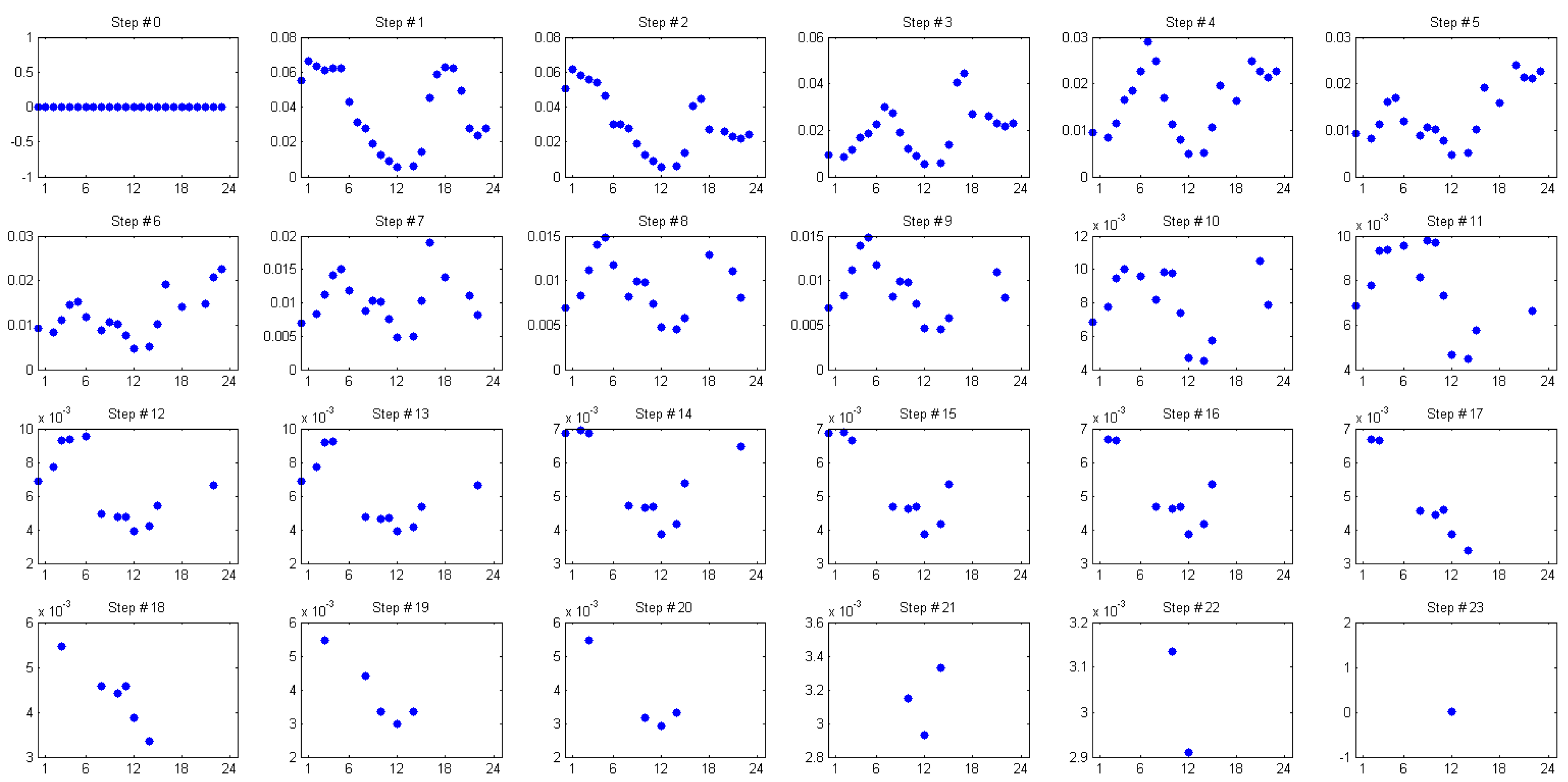
3.2. Model Construction

The model is built based on the learning data set consisting of n = 1583 days. In step zero, we construct 24 models (1) with one describing variable. Each model consists of 23 regression equations $E\left(h_p\right)=a_{0p}+a_{1p}E\left(h_q\right)$, where $p=1,\dots , 24,$ $q=1,\dots , 24$, and $p\ne q$. For each model, we calculate the MRSD (6) measure. Values of the measure are plotted in Figure 5 vs. index of the describing variable. The lowest values of the measure are mainly located between hours 11 and 15. Those models are characterized by the lowest mean relative standard deviation.

In the first step, we choose the best model—the one with the lowest MRSD. The describing variable for that model is the first chosen hour. This hour is denoted by $h_1=14$, and the model has the form $E\left(h_p\right)=a_{0p}+a_{1p}E\left(h_1\right)$. During steps 2 to 23, the choice of the describing variable is performed on the basis of another rule: the worst described hour $h_p$ is chosen. We calculate the root mean squared error (2) for each equation. The second step starts with choosing the variable with the maximum measure (2): $h_2=9$. This is the worst described variable. Now it becomes one of the describing variables. Twenty-two linear regressions with variables $E\left(h_1\right)$ and $E\left(h_2\right)$ are evaluated, and for each equation measure (2) is calculated. Other steps are processed in the same manner as step 2 until one model with 23 variables is obtained. However, the procedure can be aborted when the assumed precision is reached.

Table 2. The all ordered hours chosen by the algorithm.

Symbol	h1	h2	h3	h4	h5	h6	h7	h8	h9	h10	h11	h12
Hour	14	20	2	18	8	21	24	17	19	6	22	10
Symbol	h13	h14	h15	h16	h17	h18	h19	h20	h21	h22	h23
Hour	7	5	23	1	16	3	12	9	4	15	11

summarizes the hours chosen by the algorithm in steps 1 through 23.

3.3. Statistical Evaluation of the Model

We performed an evaluation of the statistical significance of the parameters for each regression of the model (1). The F test was used, whose statistic is the ratio of the explained variance to the unexplained variance. Obtained values of F are high, ranging from 1.9 × 10³ to 8.3 × 10⁵. The results are presented in Figure 6 on a log scale. The values of F greatly exceed critical values F*, which are in the range of 0.004—0.568 for significance level α = 0.05. The results clearly show that all of the model’s regressions are statistically significant (1).

Figure 7 shows the values of the relative standard deviation (3) for every equation of the model (1). For the first step, $\nu \left(h_p\right)$ does not exceed 7% of the average power consumption, and its mean value is about 5%. We observe a systematic decrease of $\nu \left(h_p\right)$ when going through the steps. For example, already in steps 4–6, $\nu \left(h_p\right)$ is less than 3%. In the next steps, we observe even lower values. The results indicate good and very good agreement of the models with data.

In the next step, we tested the null H₀ hypothesis regarding the agreement of the residual distribution with the normal distribution for every model equation and step. The Kolmogorov–Smirnov test (K-S test) was used. Its statistics measure the distance between the cumulative empirical distribution of the sample and the cumulative distribution function of the normal distribution. The large samples we used allowed us to precisely evaluate empirical distributions. For comparison, we utilized Marsaglia’s version of the K-S test [37]. The results of both tests were very similar. For 256 regressions, about 70.8% indicated a lack of reasons to reject the null hypothesis. The positive results increased with steps: from 30.1% for k = 1 and 70.0% for k = 4 to 100.0% for k = 12, …, 23. In about 29.2% of cases, the results of the test indicated a rejection of the H₀. It is important to note that the residual distributions in these cases did not deviate significantly from the normal distribution. The values of the skewness and kurtosis of the residual distributions are shown in Figure 8 and Figure 9.

The values of skewness are around 0, and the values of kurtosis are mostly located slightly below 3. The values of skewness are spread from −1 to 1, but from step 5 they are between −0.4 and 0.4. Kurtosis in the first steps assumes values between 2 and 4, during the next steps its values are concentrated between 2.5 and 3.5, and at the end of the procedure they are in the range of 2.6–3.0. The observed values of skewness and kurtosis indicate an approximate agreement between the distribution of random terms and a normal distribution. These results prove that the linear models were evaluated properly, and the predictions made based on them should be consistent in the whole range of independent variables.

The presented algorithm chooses and converts one described variable into the describing variable in each step. In order to obtain the model in step k, one has to go through steps 1 to k and evaluate ${{\displaystyle \sum }}_{i=1}^k\left(24-k\right)$ equations. Thus, for step k = 23, it is necessary to evaluate a total of 276 equations. On the other hand, when using the regular approach, previous steps can be skipped, but all combinations of k describing variables must be considered. Each combination requires the evaluation of 24 − k equations. Therefore, in order to build a model with k variables one has to evaluate $\left(\begin{array}{c}24\\ k\end{array}\right)\left(24-k\right)$ equations. The number of evaluated equations for each step is presented in Figure 10a for both approaches.

The number of calculated equations in the regular approach exceeds the number of equations in our model by several orders of magnitude. For example, at step number 10, those values are 27,457,584 and 185, respectively. A computer equipped with an Intel Core i7-855OU CPU and 16 GB RAM calculated the model using the regular method for about 197 h (see Figure 10, right plot). The presented algorithm required less than 1 min for the calculations.

We now compare the accuracy of model (1) with the accuracy of the models yielded by the regular method. In order to evaluate the qualities of the models, we used two measures defined by Formulas (5) and (6). The results are presented in Figure 11 for steps 3, 4, 5, and 6. The horizontal axes show mean relative standard deviations ($MRSD\mathrm{s}$) and the vertical axes show mean standard deviations ($MSD\mathrm{s}$). The blue points indicate the qualities of the models yielded by considering all the k-element subsets. The highlighted points reflect the results for model (1) and are located among the models with the best values of both measures. There are a few models that have lower values of the measures. However, these differences do not seem to be significant from a statistical point of view. In order to evaluate the accuracy of the measures used, we adopted the bootstrap method. We generated 5000 bootstrap samples, evaluated a model for each sample and calculated both measures. The 95% bootstrap confidence intervals are listed in

Table 3. The 95% bootstrap confidence intervals of MRSD and MRRSD measures for steps 3 to 6.

Step (k)	3	4	5	6
MRSD	353.08 ± 9.38	284.80 ± 9.00	236.08 ± 8.08	210.66 ± 6.96
MRRSD	0.0205 ± 0.0008	0.0170 ± 0.0007	0.0140 ± 0.0006	0.0126 ± 0.0006

for steps 3 to 6.

The results are also presented in the inset plots in Figure 11. Model (1) is indicated by a green diamond, and the 95% bootstrap regions are marked by a red color. The bootstrap regions are reflected by the 95% confidence intervals in the axes. They exceed beyond the lowest obtained values of both measures. Therefore, the obtained results show that observed differences between the best models are not statistically important. The presented model produces statistically consistent results with the best models.

4. Testing the Model

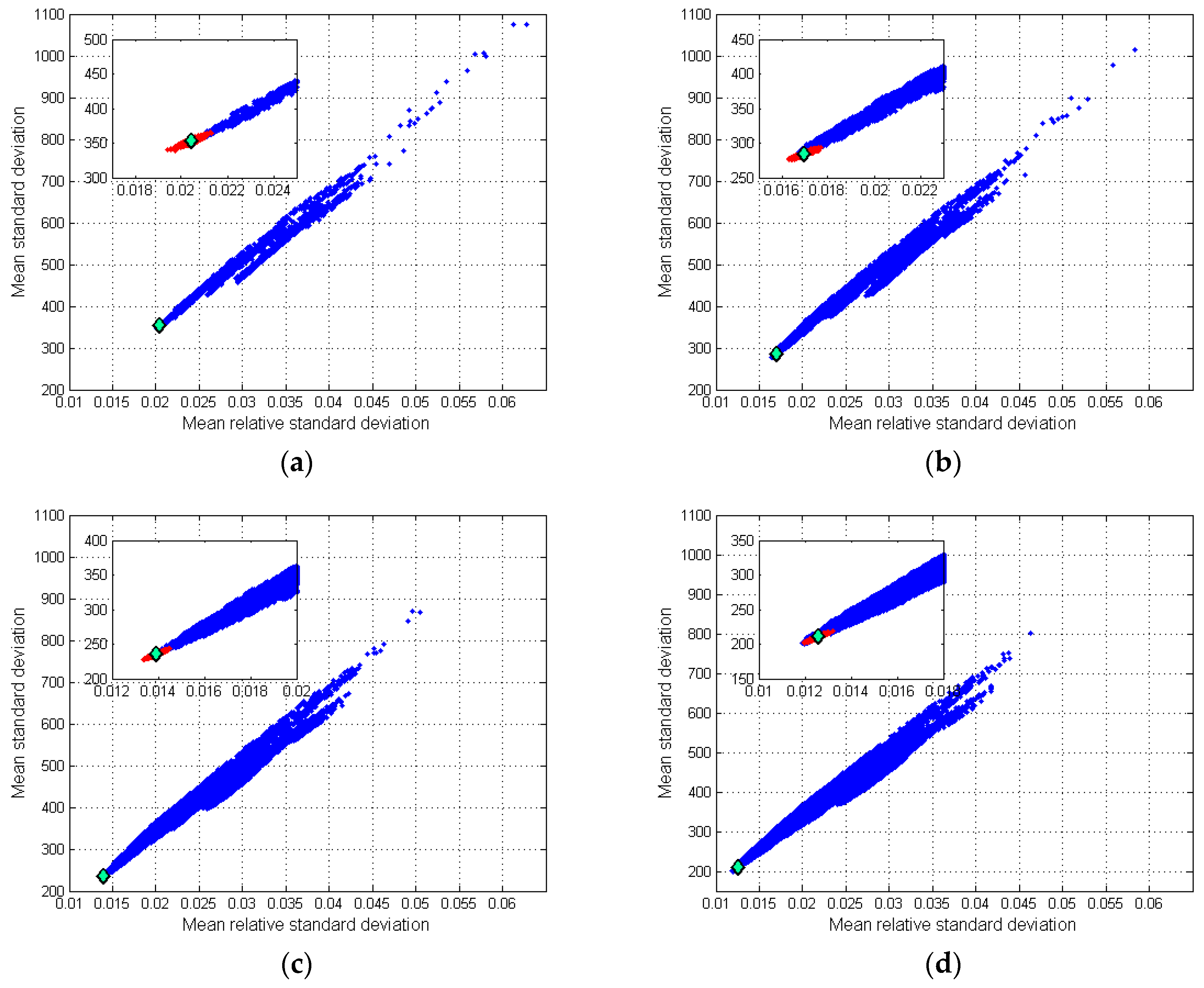
4.1. Choosing the Optimal Model

During the construction of the model, the accuracy increases with the number of steps. On the other hand, the number of described variables decreases. Therefore, with every step we obtain a model which is more accurate but has lower usefulness (describes fewer variables). The final number of describing variables is a compromise between the accuracy of the model and the number of described variables.

The values of the relative standard deviation (see Figure 7) indicate that already in step 4, the compatibility of the model with the data is very good, $\nu \left(h_p\right)<0.03$. There is only a small improvement of the precision with the next two steps. This result indicates that the model with four describing variables is the optimal model. In order to verify this result, another two measures were used: MSD and MRSD. The results for both measures are very similar to each other. The values of MSD are plotted in Figure 12.

The improvement of the measure is very substantial in the first steps and decreases thereafter. This behavior is clearly shown in the inset logarithmic plot. The value of the measure at step 4 drops by 7.3 times when compared with the dispersion of data points. During the next steps, the measure decreases systematically according to the exponential law. However, the decrease in the measure after step 4 is significantly smaller. These results point to step 4 as the optimal model with high accuracy and a small number of describing variables (20 described variables). To summarize, the algorithm chose a model with four variables defined by energy consumption at h₁ = 14, h₂ = 20, h₃ = 2, and h₄ = 18. The model consists of 20 equations and is described by the formula:

$$E\left(h_p\right)=a_{0p}+a_{1p}E\left(h_1\right)+a_{2p}E\left(h_2\right)+a_{3p}E\left(h_3\right)+a_{4p}E\left(h_4\right)+{\xi }_p$$

(8)

where $p\in \left\{5, \dots , 24\right\}.$

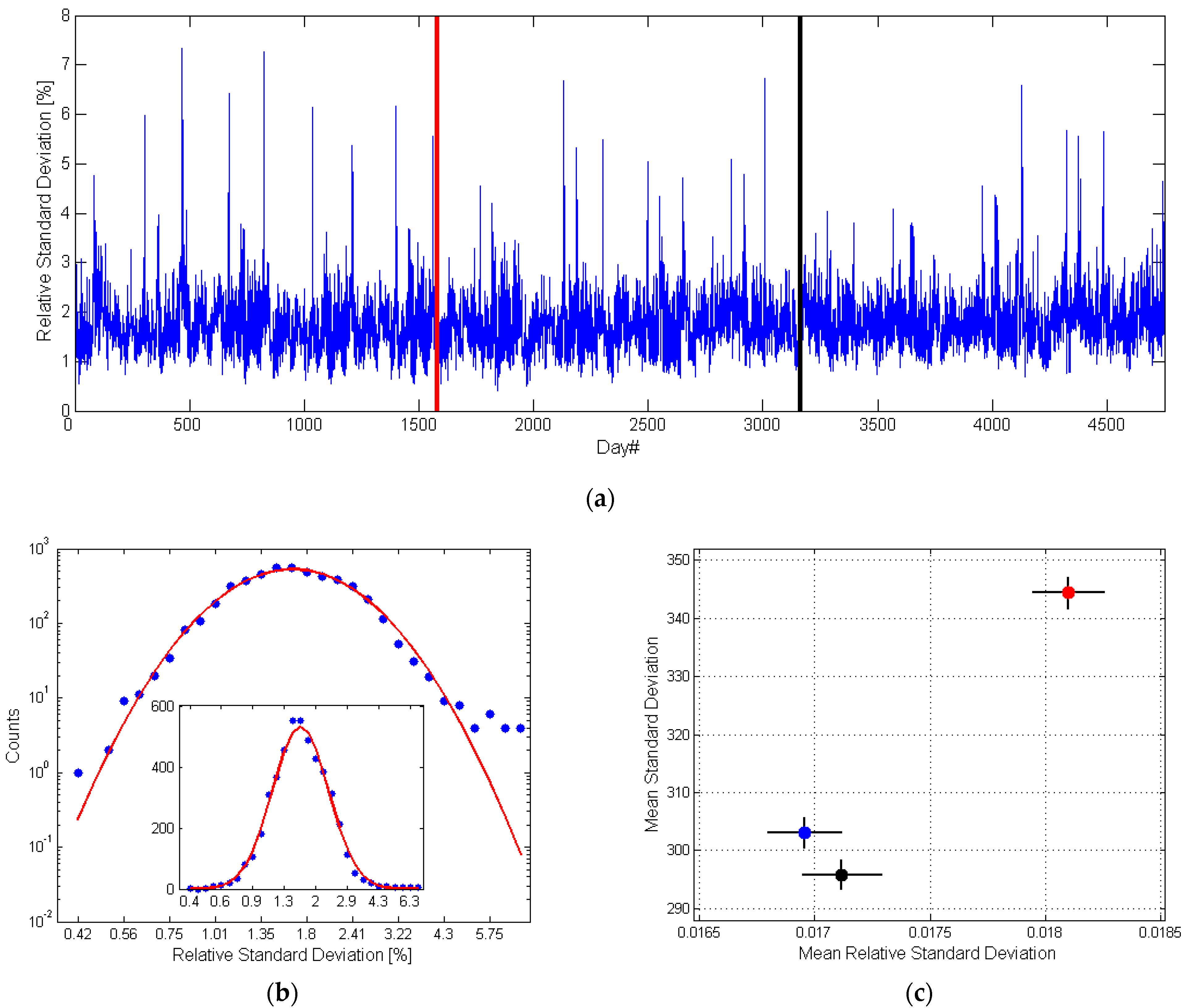
4.2. Testing the Optimal Model

The optimal model with four variables was tested on the two additional testing data sets mentioned in Table 1. For each day, the quality of the model was evaluated using two measures: absolute and relative. The measures for the model consisting of 20 equations are defined by the following formulas:

$$SD\left(i\right)=\sqrt{\frac{1}{20}{\displaystyle \sum }_{p=5}^{24}{\left(E_i\left(h_p\right)-{\widehat{E}}_i\left(h_p\right)\right)}^2}$$

(9)

$$RSD\left(i\right)=\sqrt{\frac{1}{20}{\displaystyle \sum }_{p=5}^{24}{\left(E_i\left(h_p\right)-{\widehat{E}}_i\left(h_p\right)\right)}^2}/\frac{1}{20}{\displaystyle \sum }_{p=5}^{24}{E}_i\left(h_p\right)$$

(10)

where in the sum, the following hours are omitted: from $h_1$ to $h_4$; i = 1, 2, …, N; and N denotes the number of analyzed days. Measures (9) and (10) correspond to measures (2) and (4), but the summing runs by hours instead of days. We will name them in the same fashion as the previous ones: standard deviation and relative standard deviation. The values of the measures express errors and, thus, the magnitude of the uncertainty of the results. The values of the RSD shown in % are presented for all three data sets in Figure 13.

The values of RSD indicate a very good model agreement with the data. Moreover, there is no visible trend of values of RSD when going from the learning set to the testing sets. The relative standard deviation is less than approximately 2.5% for the majority of days. The distribution is strongly asymmetric, and its right tail contains some relatively high values, shown in Figure 13 as tall spikes. We examine those values closer in the following part of this section. We investigated the logarithms of RSD. Figure 13b shows that their distribution is Gaussian, and thus the distribution of errors is log-normal. To ensure consistency between plots, the numbers on the horizontal axis represent RSD values rather than log(RSD) values. The outer bottom left plot shows the distribution of counts on a log scale. There are outliers corresponding to the tall spikes. The results were grouped for each data set, and mean values of the standard deviation and relative standard deviation were calculated. The results are provided in

Table 4. Mean errors and their standard deviations for learning and testing data sets.

Measure	Learning Set	Testing Set I	Testing Set II
MRSD	0.0172 ± 0.0018	0.0169 ± 0.0017	0.0182 ± 0.0017
RSD [MWh]	296.5 ± 2.8	302.8 ± 2.7	344.2 ± 2.7

, and are plotted together with errors in Figure 13c for each data set. Errors of measures are expressed as their standard deviations. The vales for the learning and first testing sets are very close to each other. The differences do not exceed one (for MRSD) and two (for MSD) standard deviations. One can conclude that the results for those two data sets are statistically compatible. For the second testing set, we obtained slightly higher values of both measures. However, the values of both measures for the third data set exceed the values for the learning data set by approximately 5% and 16%. Moreover, the number of tall spikes in the third data set does not exceed the number of such spikes in the remaining data sets.

4.3. Typical Days and Outliners

We show the model values and empirical data for selected days in Figure 14. Days are chosen in pairs from the first and second testing data sets. The chosen dates correspond to each other in both data sets:

• First Thursday of March;
• First day of school holidays;
• Last Monday of school holidays;
• Tuesday in the middle of October;
• Friday in the middle of January;
• Christmas;
• First Wednesday of December.

A description of the selected days and the compliance level with data measured by the relative standard deviation (RSD) is presented in

Table 5. The selected 14 days with the RSD errors in %.

No	Date Testing Set I	RSD (%)	Date Testing Set II	RSD (%)	Weekday	Figure 14
1	7 March 2013	0.882	2 March 2017	1.139	Thursday	(a), (b)
2	1 July 2012	2.671	2 July 2017	1.958	Sunday	(c), (d)
3	27 August 2012	1.736	28 August 2017	1.440	Monday	(e), (f)
4	14 October 2014	1.366	16 October 2018	2.069	Tuesday	(g), (h)
5	16 January 2015	1.553	18 January 2019	1.052	Friday	(i), (j)
6	25 December 2015	1.858	25 December 2020	1.830	Friday	(k), (l)
7	2 December 2015	1.725	2 December 2020	1.386	Wednesday	(m), (n)

.

Although the presented plots are for different days of the week, seasons, and environmental conditions (thus having various shapes), the model describes the data very well. The shapes of the empirical and theoretical plots are similar to each other. Looking at Figure 14 it can be seen that theoretical data points are very close to empirical data points, and often overlap. For some hours, slightly greater differences are visible, but the mean values of RSD are mainly below 2%. One can conclude that the level of uncertainty for the presented days is low.

In this part of the paper, we examine days with the highest values of the RSD measure, shown in Figure 13 as tall spikes. We discussed all spikes higher than 5%, and they are described in

Table 6. The days described by the model with the quality RSD greater than 5%. Learning set, testing set I, and testing set II are separated by horizontal lines.

Day#	Date	RSD (%)	Description
306	1 November 2008	5.972	All Saints’ Day
468	12 April 2009	7.330	Easter
671	1 November 2009	6.420	All Saints’ Day
825	4 April 2010	7.254	Easter
1036	1 November 2010	6.149	All Saints’ Day
1210	24 April 2011	5.379	Easter
1401	1 November 2011	6.170	All Saints’ Day
1560	8 April 2012	5.553	Easter
2132	1 November 2013	6.673	All Saints’ Day
2185	24 December 2013	5.333	Christmas Eve
2302	20 April 2014	5.484	Easter
2497	1 November 2014	5.036	All Saints’ Day
2862	1 November 2015	5.091	All Saints’ Day
3009	27 March 2016	6.717	Easter
4129	21 April 2019	6.578	Easter
4323	1 November 2019	5.672	All Saints’ Day
4376	24 December 2019	5.546	Christmas Eve
4486	12 April 2020	5.660	Easter

.

All the observed tall spikes are related to the biggest religious holidays in Poland, which are also public holidays. Christmas is the biggest holiday in Poland. Christmas Eve cannot be considered as a regular working day. The working hours are usually reduced, and people celebrate with holiday supper. All Saints’ Day is a public holiday during which many people travel to visit family graves. On Easter Sunday, families celebrate with breakfast. All the observed days cannot be considered as typical days from the energy consumption point of view. Energy demands and daily time series are different from those for regular days. The model distinguishes those days by high RSD values. The model integrates this feature obtained during learning and propagates it precisely onto the testing data sets. The developed model can be used to distinguish nontypical days from the electricity consumption point of view.

5. Discussion

5.1. Novelty of the Presented Approach

When building models on electricity consumption, numerous works [11,12,13,14] focus on the effect of external factors (humidity, temperature, sunshine, etc.) on energy consumption. Meanwhile, these factors not only do not change rapidly from hour to hour, but often remain at the same level throughout the day. On the other hand, other works [12,28] focus on the determination of energy consumption based on past energy consumption (autoregressive models). We, meanwhile, focus on modeling daily runs determined by energy consumption at specific fixed hours, regardless of external factors.

The proposed multiple-equation linear regression model is an iterative one, and consists of a series of steps. The model is modified in each step. the novelty of this approach is that it allows us to model energy consumptions for the entire day using only a few selected hours. It has been shown that just four hours are sufficient to describe the energy consumption for the remaining hours with high precision, no worse than other models involving many external factors, which increases the cost of the model. Our previous work [5] with the use of (approximately) 35 variables, their selection, and optimization of many parameters led to results with errors above 3%—larger than those obtained when using this new model in step 4, i.e., below 2.5%.

5.2. Selection of the Best Variable Set

The algorithm presented in this paper is iterative and consists of a series of steps. The model is modified in each step. At the first step, the algorithm chooses the best describing variable. This choice is made based on 24 models, each consisting of 23 regressions. The model with the lowest mean relative standard deviation, MRSD, is selected. The first chosen hour is a describing variable for that model. One can say that this variable describes the remaining variables in the best possible way. Starting from the second step, the algorithm chooses the variable described as the worst in the previous step according to the relative standard deviation (RSD). This variable becomes another describing variable. One can say that this variable is related to the other describing variables in the worst way. Using this approach, other models are constructed, each containing a set of variables that are less related to one another. As we have proven, this procedure leads to the best model (see Figure 11). We verified that choosing variables based on the correlation matrix did not produce good results.

The algorithm chose t₁ = 14 in the first step. As can be seen in Figure 5, there are some points (t = 11, 12, 13, 15) with very similar values of measure. We investigated them and found that choosing one of the above points only slightly lowered the quality of the model. The remaining hours were chosen for the model in a similar way (see Table 2). On the other hand, the starting hours with significantly higher MRSD led to models of significantly lower quality. Figure 15 illustrates this fact. The green point indicates our optimal model for t₁ = 14, and the red points denote models with different starting hours. Models with the starting hours mentioned above (t = 11, 12, 13, 15) are located close to the green point but characterized by the worse values of both measures.

The described algorithm allows for a quality measure to be chosen. The obtained results were confirmed using the additional measures listed in Section 3.1. The choice of the first hour was performed using the MRRSD measure (7) instead of MRSD (6). For steps 2 onward, measure (3) was replaced by measure (4). Measures (4) and (7) are based on the calculation of the relative residual value for each empirical data point. In contrast, measures (3) and (6) are based on the mean values of empirical data points. The replacement of measure led to the same results.

5.3. The Issue of Overfitting

The described algorithm allows the procedure to be stopped at any step. A decision can be taken based on the observed errors. The presented results were obtained when the procedure was stopped at step 4 when $\nu \left(h_p\right)<0.03$. In the previous step, the model uncertainty was greater and reached 0.05. That model contained only three variables, and the remaining hours were described with greater errors. On the other hand, one could proceed to the next steps, e.g., for k = 6, $\nu \left(h_p\right)<0.0025$ and for k = 8, $\nu \left(h_p\right)<0.0015$ (see Figure 7). Results would be more accurate, but more data would be used and less described. In this way, by reducing the error too much, the model would be overtrained. In the case of our model, early stopping should be used to reduce the chance of overfitting.

Even when the overfitted model does not contain an excessive number of parameters, it is to be expected that the model will perform less well on the testing data set than on the learning set. In our study, this phenomenon did not take place. We showed that on the learning set, mean relative error MRSD is approximately 1.72%, while on the testing sets it is 1.69% and 1.82% (see Table 4). Moreover, the mean absolute error MSD on the learning set is equal to about 297 MWh, while on the testing sets it is about 303 MWh and 344 MWh. The slightly greater error observed on the second learning set is related to the distant time horizon (a few years), in which we observe a slight overall increase in energy consumption. This increase is cancelled out by using relative error. We also ensured that the distributions of the model residuals are normal by investigating their kurtosis and skewness.

6. Summary

In this work, a new approach to modeling hourly energy consumption was presented. We proposed a multiple-equation linear regression model. The approach presented herein allows for the modeling of energy consumptions for the entire day using only a few selected hours. This model was verified in detail using statistical methods. The results are summarized in the following items.

• All the model equations are statistically significant and the agreement with empirical data is very high. In the first step, the relative error of the model does not exceed 7% and decreases to below 3% in step 4.
• For approximately 71% of equations, the residual distribution is fully compatible with a Gaussian distribution. The observed differences in the remaining cases are very small.
• When compared to the standard approach based on the analysis of all possible combinations of describing hours, the model yields the best result.
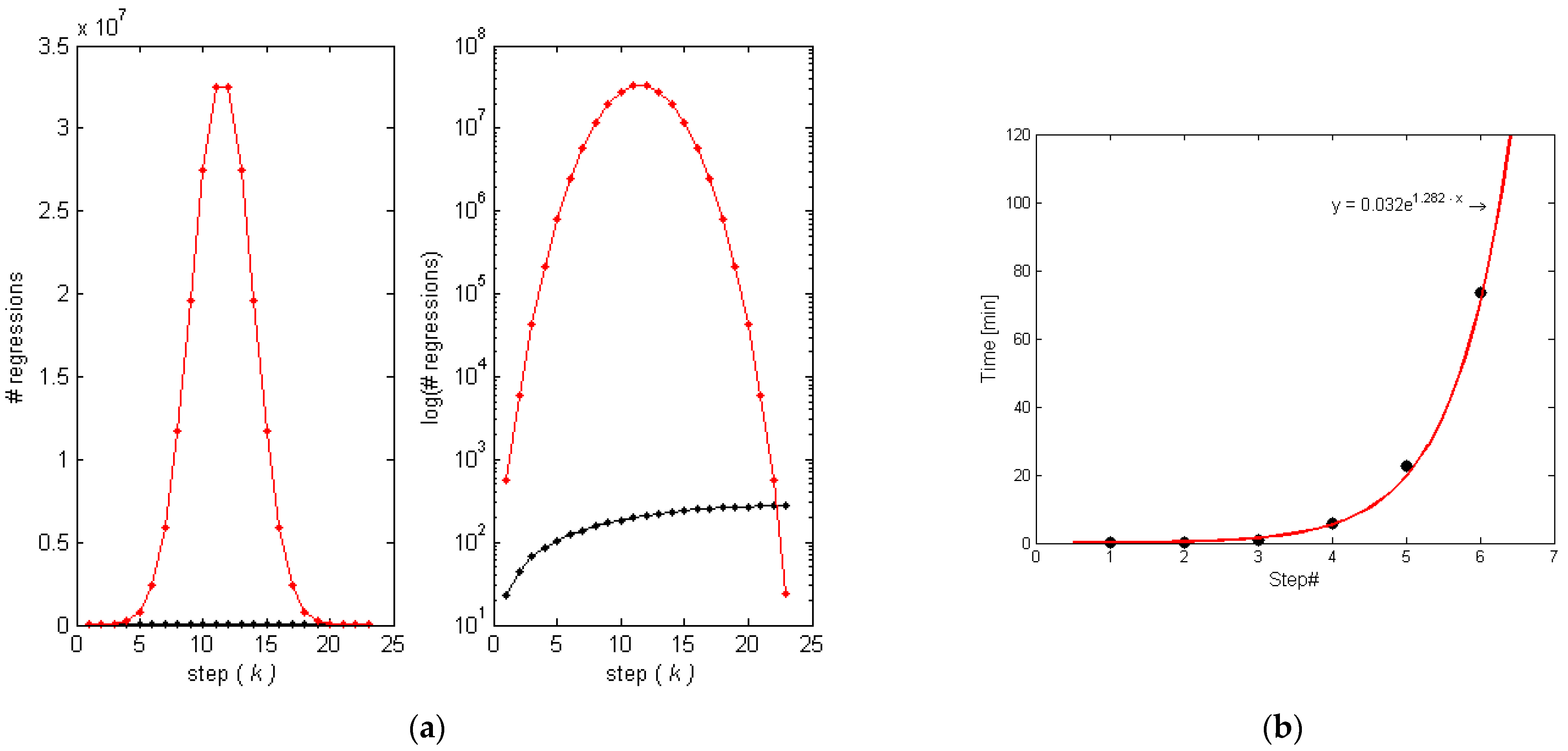
• The algorithm is very fast. With limited computation power it detects the optimal describing variables, and calculates the parameters of the model.
• Only four hours are sufficient to describe the energy consumption for the remaining hours with high precision. We obtained a mean relative uncertainty of 1.72% in the learning data set, and 1.69% and 1.82% in the two testing data sets.
• The highest daily errors of the model do not exceed 7.5%, but the majority of days are described with an uncertainty better than 2.5%.
• Days for which the model has the highest uncertainty, greater than 5%, are public holidays in Poland. They exhibit nontypical energy consumption.

The authors can indicate further directions for studies implementing the presented method.

• The detection of days with nontypical energy consumption. The values of the model quality measures are high for such days. Detecting these days is critical, not only for forecasting purposes, but also for optimizing the energy supplier system.
• The classification of days based on the energy consumption profile is another issue that is of great interest. On the other hand, the classification and clustering of the daily energy consumption require the consideration of 24 variables. The proposed method allows for a significant reduction of the space dimension.
• The standard methods of long-term forecasting deal with the forecasting of energy consumption, which exhibits strong daily periodicity. At the same time, forecasting energy consumption at separate hours allows for the elimination of problems arising from such periodicity. The model will allow for the reconstruction of the energy consumption for the entire day based on the forecasted energy demand for only a few hours.

References

- Alfares, H.K.; Nazeeruddin, M. Electric load forecasting: Literature survey and classification of methods. Int. J. Syst. Sci. 2002, 33, 23–34. [Google Scholar] [CrossRef]
- Feinberg, E.A.; Genethliou, D. Load forecasting. In Applied Mathematics for Restructured Electric Power Systems. Power Electronics and Power Systems; Chow, J.H., Wu, F.F., Momoh, J., Eds.; Springer: Boston, MA, USA, 2005; pp. 269–285. [Google Scholar] [CrossRef]
- Hong, T. Energy forecasting: Past, present, and future. Int. J. Appl. Forecast. 2014, 32, 43–48. [Google Scholar]
- Hong, T.; Gui, M.; Baran, M.E.; Willis, H.L. Modeling and forecasting hourly electric load by multiple linear regression with interactions. In Proceedings of the 2010 Power and Energy Society General Meeting, Minneapolis, MN, USA, 25–29 July 2010; pp. 1–8. [Google Scholar]
- Karpio, K.; Łukasiewicz, P.; Nafkha, R. Regression Technique for Electricity Load Modeling and Outlined Data Points Explanation. In Advances in Soft and Hard Computing; Advances in Intelligent Systems and, Computing; Pejaś, J., El Fray, I., Hyla, T., Kacprzyk, J., Eds.; Springer: Cham, Switzerland, 2019; Volume 889, pp. 56–67. [Google Scholar] [CrossRef]
- Lindberg, K.B.; Seljom, P.; Madsen, H.; Fischer, D.; Korpas, M. Long-term electricity load forecasting: Current and future trends. Util. Policy 2019, 58, 102–119. [Google Scholar] [CrossRef]
- Rajakovic, N.L.; Shiljkut, V.M. Long-term forecasting of annual peak load considering effects of demand-side programs. J. Mod. Power Syst. Clean Energy 2018, 6, 145–157. [Google Scholar] [CrossRef]
- Mojica, J.L.; Petersen, D.; Hansen, B.; Powell, K.M.; Hedengren, J.D. Optimal combined long-term facility design and short-term operational strategy for CHP capacity investments. Energy 2017, 118, 97–115. [Google Scholar] [CrossRef]
- Torkzadeh, R.; Mirzaei, A.; Mirjalili, M.M.; Anaraki, A.S.; Sehhati, M.R.; Behdad, F. Medium term load forecasting in distribution systems based on multi linear regression & principal component analysis: A novel approach. In Proceedings of the 19th Electrical Power Distribution Networks (EPDC), Tehran, Iran, 6–7 May 2014; pp. 66–70. [Google Scholar]
- Taleb, I.; Guerard, G.; Fauberteau, F.; Nguyen, N. A Flexible Deep Learning Method for Energy Forecasting. Energies 2022, 15, 3926. [Google Scholar] [CrossRef]
- Elkamel, M.; Schleider, L.; Pasiliao, E.; Diabat, A.; Zheng, Q.P. Long-Term Electricity Demand Prediction via Socioeconomic Factors—A Machine Learning Approach with Florida as a Case Study. Energies 2020, 13, 3996. [Google Scholar] [CrossRef]
- Angelopoulos, D.; Siskos, Y.; Psarras, J. Disaggregating time series on multiple criteria for robust forecasting: The case of long-term electricity demand in Greece. Eur. J. Oper. Res. 2019, 275, 252–265. [Google Scholar] [CrossRef]
- Abu-Shikhah, N.; Elkarmi, F.; Aloquili, O. Medium-Term Electric Load Forecasting Using Multivariable Linear and Non-Linear Regression. Smart Grid Renew. Energy 2011, 2, 126–135. [Google Scholar] [CrossRef]
- Eneje, I.S.; Fadare, D.A.; Simolowo, O.E.; Falana, A. Modelling and Forecasting Periodic Electric Load for a Metropolitan City in Nigeria. Afr. Res. Rev. 2012, 6, 101–115. [Google Scholar] [CrossRef]
- Bruhns, A.; Deurveilher, G.; Roy, J.S. A non-linear regression model for midterm load forecasting and improvements in seasonality. In Proceedings of the 15th Power Systems Computation Conference, Liege, Belgium, 22–26 August 2005; pp. 22–26. [Google Scholar]
- Charytoniuk, W.; Chen, M.S.; Van Olinda, P. Nonparametric regression based short-term load forecasting. IEEE Trans. Power Syst. 1998, 13, 725–730. [Google Scholar] [CrossRef]
- Dudek, G. Pattern-based local linear regression models for short-term load forecasting. Electr. Power Syst. Res. 2016, 130, 139–147. [Google Scholar] [CrossRef]
- Sood, R.; Koprinska, I.; Agelidis, V.G. Electricity load forecasting based on autocorrelation analysis. In Proceedings of the 2010 International Joint Conference on Neural Networks (IJCNN), Barcelona, Spain, 18–23 July 2010; pp. 1–8. [Google Scholar] [CrossRef]
- Fan, S.; Hyndman, R.J. Short-term load forecasting based on a semi-parametric additive model. IEEE Trans. Power Syst. 2012, 27, 134–141. [Google Scholar] [CrossRef]
- Sharma, P.; Said, Z.; Kumar, A.; Nižetić, S.; Pandey, A.; Hoang, A.T.; Huang, Z.; Afzal, A.; Li, C.; Le, A.T.; et al. Recent Advances in Machine Learning Research for Nanofluid-Based Heat Transfer in Renewable Energy System. Energy Fuels 2022, 36, 6626–6658. [Google Scholar] [CrossRef]
- Said, Z.; Nguyen, T.H.; Sharma, P.; Li, C.; Ali, H.M.; Nguyen, V.N.; Pham, V.V.; Ahmed, S.F.; Van, D.N.; Truong, T.H. Multi-attribute optimization of sustainable aviation fuel production-process from microalgae source. Fuel 2022, 324, 124759. [Google Scholar] [CrossRef]
- Jihoon, M.; Yongsung, K.; Minjae, S.; Eenjun, H. Hybrid Short-Term Load Forecasting Scheme Using Random Forest and Multilayer Perceptron. Energies 2018, 11, 3283. [Google Scholar] [CrossRef]
- Dahl, M.; Brun, A.; Kirsebom, O.S.; Gorm, B.; Andresen, G.B. Improving Short-Term Heat Load Forecasts with Calendar and Holiday Data. Energies 2018, 11, 1678. [Google Scholar] [CrossRef]
- Ping-Huan, K.; Chiou-Jye, H. A High Precision Artificial Neural Networks Model for Short-Term Energy Load Forecasting. Energies 2018, 11, 213. [Google Scholar] [CrossRef]
- Campo, R.; Ruiz, P. Adaptive weather-sensitive short term load forecast. IEEE Trans. Power Syst. 1987, 2, 592–598. [Google Scholar] [CrossRef]
- Ghosh, S. Univariate time-series forecasting of monthly peak demand of electricity in northern India. Int. J. Indian Cult. Bus. Manag. 2008, 1, 466–474. [Google Scholar] [CrossRef]
- Mirasgedis, S.; Sarafidis, Y.; Georgopoulou, E.; Lalas, D.P.; Moschovits, M.; Karagiannis, F.; Papakonstantinou, D. Models for Mid-Term Electricity Demand Forecasting Incorporating Weather Influences. Energy 2006, 31, 208–227. [Google Scholar] [CrossRef]
- Hong, T.; Wilson, J.; Xie, J. Long Term Probabilistic Load Forecasting and Normalization with Hourly Information. IEEE Trans. Smart Grid 2014, 5, 456–462. [Google Scholar] [CrossRef]
- Chen, Y.; Luh, P.B.; Guan, C.; Zhao, Y.; Michel, L.D.; Coolbeth, M.A.; Friedland, P.B.; Rourke, S.J. Short-term load forecasting: Similar day-based wavelet neural networks. IEEE Trans. Power Syst. 2010, 25, 322–330. [Google Scholar] [CrossRef]
- Ailing, Y.; Weide, L.; Xuan, Y. Short-term electricity load forecasting based on feature selection and Least Squares Support Vector Machines. Knowl.-Based Syst. 2019, 163, 159–173. [Google Scholar] [CrossRef]
- Li, X.; Zhao, B.; Ji, W.; Jing, X.; He, Y. Short-Term Electricity Load Forecasting Model Based on EMD-GRU with Feature Selection. Energies 2019, 12, 1140. [Google Scholar] [CrossRef]
- Hong, T. Short Term Electric Load Forecasting. Ph.D. Thesis, North Carolina State University, Raleigh, NC, USA, 20 November 2010. [Google Scholar]
- Hyndman, R.J.; Ahmed, R.A.; Shang, H.L. Optimal combination forecasts for hierarchical time-series. Comput. Stat. Data Anal. 2011, 55, 2579–2589. [Google Scholar] [CrossRef]
- Pang, Y.; Jin, C.; Zhou, X.; Guo, N.; Zhang, Y. Hierarchical Electricity Demand Forecasting by Exploring the Electricity Consumption Patterns. In Proceedings of the 7th International Conference on Pattern Recognition Applications and Methods (ICPRAM 2018), Madeira, Portugal, 16–18 January 2018; pp. 576–581. [Google Scholar]
- Karpio, K.; Łukasiewicz, P.; Nafkha, R.; Orłowski, A. Description of Electricity Consumption by Using Leading Hours Intra-day Model. In Computational Science—ICCS 2021. Lecture Notes in Computer Science; Paszynski, M., Kranzlmüller, D., Krzhizhanovskaya, V.V., Dongarra, J.J., Sloot, P.M., Eds.; Springer: Cham, Switzerland, 2021; Volume 12745, pp. 392–404. [Google Scholar] [CrossRef]
- Polskie Sieci Elektroenergetyczne. Available online: http://www.pse.pl (accessed on 15 January 2023).
- Marsaglia, G.; Tsang, W.W.; Wang, J. Evaluating Kolmogorov’s Distribution. J. Stat. Softw. 2003, 8, 1–4. [Google Scholar] [CrossRef]