Kernel Function-Based Inverting Algorithm for Structure Parameters of Horizontal Multilayer Soil

Abstract

A multilayer soil structure model is fundamental to design grounding systems. A new method is presented to invert the structure parameters of horizontal multilayer soil. The structure parameters of soil are determined by analyzing the kernel function of the integral equation of the apparent resistivity. The essence of the proposed method avoids the difficulties encountered in general optimization methods; namely, the calculation of the apparent resistivity and its derivative.

1. Introduction

When installing an underground system, knowledge of the local underground structure is essential. Parameters of the stratum structure are indispensable data for field or circuit level simulations of the underground system. This is because a poorly designed grounding system cannot guarantee the safety of human lives as well as expensive equipment [1,2].

An analysis of the underground structure is mainly based on an $N$-layer structure, in which the strata are formed horizontally. This is because in the process of formation of strata, in most strata, new sediments are often formed as new sediments are horizontally stacked on top of existing strata. Therefore, the problem of estimating the parameters of a land structure composed of $N$ layers results in an unconstrained nonlinear minimization problem of estimating $2N-1$ parameters. It is only necessary to determine $N$ resistivities and $N-1$ layer thicknesses [3,4].

This study can be classified into two categories. The first one is using deterministic optimization algorithms, the advantage of which is high efficiency, but it normally requires accurate derivatives of the objective function to accelerate the convergence procedure. The other type is the non-deterministic optimization algorithms, such as the artificial neural networks (ANN) and genetic algorithms (GA). Over the past few decades, new methods based on artificial intelligence have been applied in various fields. Recently, deep learning systems based on artificial intelligence have been put in the limelight; they are popular in all fields. ANNs are basically models that learn from data, similar to biological systems in the brain [4]. Recently, with the help of massive amounts of data and ultra-fast processors that can process them, ANNs have been rapidly developing. In addition, artificial neural networks of various structures are being used in the fields of parameter estimation and ground structure prediction. For the deterministic optimization algorithm methods, various optimization algorithms have been used to solve this problem, but the most used method is to set an objective function and minimize the objective function while adjusting the parameters. The objective function uses the apparent soil resistivity, which is found by the error between the measured value and the theoretical value. The measurement of apparent soil resistivity mainly uses Wenner’s four-electrode method.

One of the most important parts of the deterministic optimization technique is the calculation of the apparent resistivity, which is a derivative of different combinations of soil parameters. Each update of the parameters requires calculating the theoretical apparent resistivity and its derivative, but it is difficult to perform infinite integrations including the Bessel function. Nondeterministic optimization algorithms avoid the difficulties mentioned by deterministic optimization techniques but have difficulties in determining the ANN type and its hyperparameters. The type of ANN and the hyperparameters of these methods produce completely different results and there are no rules determining them [3,4,5]. Many published papers have aimed to address these issues. Bo Zhang used Prony’s method to improve the computational number of theoretical values [3]. J. Zou especially proposed a two-stage algorithm to avoid calculating the apparent soil resistivity each time a parameter is updated [6,7,8,9,10].

The method proposed in this paper uses the kernel function of the apparent resistance integration. The kernel function is included in the formula for calculating the apparent earth resistivity. Additionally, the kernel function consists of soil composition parameters. That is, in the general optimization method, in the process of minimizing the error function, the assumed variable approaches the actual value and the kernel function becomes accurate. J. Zou has proposed a method for estimating the kernel function directly from the measured data. In this way, he avoided calculating the apparent soil resistivity every time the parameters were updated, reducing the amount of calculations [6,7,8,9,10]. In this paper, we propose a method for calculating soil parameters analytically using a kernel function rather than a general optimization method. In other words, after estimating the kernel function with the method proposed by J. Zou, we propose a method to obtain the site parameters by analyzing the characteristics of the kernel function. The method proposed in this paper is also a two-step algorithm. In the first step, the kernel function of the apparent resistivity integral equation was solved based on J. Zou’s method. A method of linearizing the nonlinear equation thus derived was proposed, and the underdetermined system was solved using the QR decomposition method. In the second step, we propose a new method to determine soil parameters using the properties of the kernel function of the apparent resistivity integral.

In this paper, a new method is presented to invert the parameter of horizontal multilayer soil. The key point is to bypass the forementioned difficulties in general optimization techniques. The contributions of this paper can be summarized as follows. First, it avoids repetitive calculation of the apparent resistivity with different parameters to fit the measured data, saving considerable computational demand. Second, there is no need for derivatives of optimized expressions that are difficult to obtain. To the knowledge of the authors, there are no articles reporting approaches for inverting soil parameters as an analytical method.

The composition of this paper is as follows: Section 2 presents the calculation and measurement method of the apparent soil resistivity, and Section 3 shows how to invert the kernel function and presents a method of linearizing the nonlinear system that occurs during inversion. Section 4 proposes a method for analytically inverting soil parameters using the properties of the kernel function. Section 5 presents numerical examples of two- and four-story structures to check their applicability in the case of various soil structures. Finally, a conclusion is presented.

2. Apparent Soil Resistivity

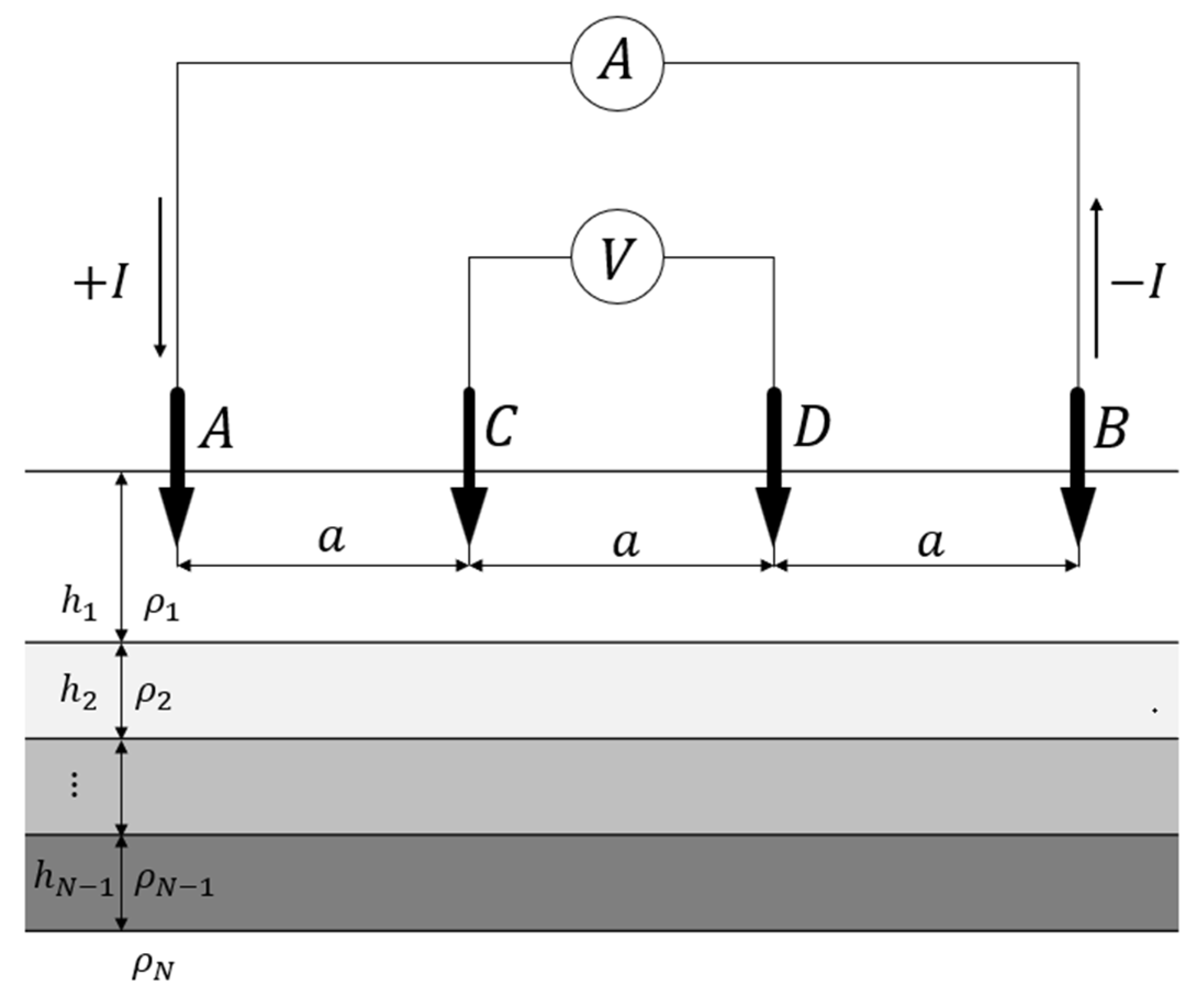
2.1. Measurement of Apparent Soil Resistivity Using the Wenner Method

The general soil resistivity measurement technique is a modified technique of the equal-spaced four-electrode method first proposed by Frank Wenner. In this method, to interpret the problem easily, it is assumed that each layer of the earth is horizontal and that each layer is formed with the same resistivity [1,2,3,4].

Figure 1 shows the arrangement of the electrodes in Wenner’s four-electrode method, where the potential electrodes C and D are placed inside on the straight line of the measurement line and the current electrodes A and B are installed outside. Additionally, the distance, a, between the measuring electrodes of A-C, C-D and D-B is equally spaced. The earth resistance, $R$, is calculated by injecting a current, I, into the external current electrode and measuring the potential difference between the internal potential electrodes. The earth resistance, $R$, is proportional to the apparent soil resistivity, and when the electrode spacing is $a$, the apparent soil resistivity, ${\mathsf{\rho }}^m\left(\mathsf{\Omega }\mathrm{m}\right)$, can be expressed as (1) in the case of the Wenner method [3].

$${\mathsf{\rho }}^m=2\mathsf{\pi }aR.$$

(1)

The apparent resistivity is the name given to the resistivity measured on the surface of the earth, and the superscript ‘m’ of $\rho$ in (1) indicates the value obtained by measuring. In Figure 1, $h_i\left(i=1,2,\dots N-1\right)$ and ${\mathsf{\rho }}_i\left(i=1,2,\dots ,N\right)$ represent the depth and resistivity of each soil layer, respectively.

2.2. Theoretical Apparent Soil Resistivity Calculation

If the depth, $h_i\left(i=1,2,\dots ,N-1\right)$, and the soil resistivity, ${\mathsf{\rho }}_i\left(i=1,2,\dots ,N\right)$, of each layer are known in the soil structure, the theoretical formula for calculating the apparent soil resistivity is as follows [7,11,12,13]:

$${\mathsf{\rho }}_a={\mathsf{\rho }}_1\left\{1+2a{{\displaystyle \int }}_0^{\infty }f\left(\mathsf{\lambda }\right)[J_0(\mathsf{\lambda }a)-J_0(2\mathsf{\lambda }a)]d\mathsf{\lambda }\right\},$$

(2)

where $a$ is the electrode spacing, $J_0\left(\mathsf{\lambda }a\right)$ is the first kind of zero-order Bessel function, and the kernel function $f\left(\mathsf{\lambda }\right)$ is defined as:

$$f\left(\mathsf{\lambda }\right)={\mathsf{\alpha }}_1\left(\mathsf{\lambda }\right)-1$$

(3)

$${\mathsf{\alpha }}_1\left(\mathsf{\lambda }\right)=1+\frac{2k_1\left(\mathsf{\lambda }\right)e^{-2\mathsf{\lambda }{h}_1}}{1-k_1\left(\mathsf{\lambda }\right)e^{-2\mathsf{\lambda }{h}_1}}, k_1\left(\mathsf{\lambda }\right)=\frac{{\mathsf{\rho }}_2{\mathsf{\alpha }}_2\left(\mathsf{\lambda }\right)-{\mathsf{\rho }}_1}{{\mathsf{\rho }}_2{\mathsf{\alpha }}_2\left(\mathsf{\lambda }\right)+{\mathsf{\rho }}_1}$$

$${\mathsf{\alpha }}_2\left(\mathsf{\lambda }\right)=1+\frac{2k_2\left(\mathsf{\lambda }\right)e^{-2\mathsf{\lambda }{h}_2}}{1-k_2\left(\mathsf{\lambda }\right)e^{-2\mathsf{\lambda }{h}_2}}, k_2\left(\mathsf{\lambda }\right)=\frac{{\mathsf{\rho }}_3{\mathsf{\alpha }}_3\left(\mathsf{\lambda }\right)-{\mathsf{\rho }}_2}{{\mathsf{\rho }}_3{\mathsf{\alpha }}_3\left(\mathsf{\lambda }\right)+{\mathsf{\rho }}_2}$$

$${\mathsf{\alpha }}_{N-2}\left(\mathsf{\lambda }\right)=1+\frac{2k_{N-2}\left(\mathsf{\lambda }\right)e^{-2\mathsf{\lambda }{h}_{N-2}}}{1-k_{N-2}\left(\mathsf{\lambda }\right)e^{-2\mathsf{\lambda }{h}_{N-2}}}, k_{N-2}\left(\mathsf{\lambda }\right)=\frac{{\mathsf{\rho }}_{N-1}{\mathsf{\alpha }}_{N-1}\left(\mathsf{\lambda }\right)-{\mathsf{\rho }}_{N-2}}{{\mathsf{\rho }}_{N-1}{\mathsf{\alpha }}_{N-1}\left(\mathsf{\lambda }\right)+{\mathsf{\rho }}_2}$$

$${\mathsf{\alpha }}_{N-1}\left(\mathsf{\lambda }\right)=1+\frac{2k_{N-1}\left(\mathsf{\lambda }\right)e^{-2\mathsf{\lambda }{h}_{N-1}}}{1-k_{N-1}\left(\mathsf{\lambda }\right)e^{-2\mathsf{\lambda }{h}_{N-1}}}, k_{N-1}\left(\mathsf{\lambda }\right)=\frac{{\mathsf{\rho }}_N-{\mathsf{\rho }}_{N-1}}{{\mathsf{\rho }}_N+{\mathsf{\rho }}_{N-1}}$$

3. Inversion of the Kernel Function

3.1. Inversion of the Kernel Function Using Apparent Soil Resistivity

It is known that the kernel function decreases exponentially as expected from (3) and can be approximated as follows [14]:

$$f\left(\mathsf{\lambda }\right)\simeq {{\displaystyle \sum }}_{k=1}^N{b}_k{e}^{-c_k\mathsf{\lambda }},$$

(4)

where $b_k$ and $c_k$ are constants.

Using Lipschitz’s integral,

$${{\displaystyle \int }}_0^{\infty }{e}^{-\mathsf{\lambda }\mid c\mid }{J}_0\left(\mathsf{\lambda }l\right)d\mathsf{\lambda }=\frac{1}{\sqrt{c^2+l^2}},$$

(5)

${\mathsf{\rho }}_a$ in (2) can be approximated as follows.

$${\mathsf{\rho }}_a\simeq {\mathsf{\rho }}_1\left\{1+2a{{\displaystyle \sum }}_{k=1}^N{b}_k\left[\frac{1}{\sqrt{c_k^2+a^2}}-\frac{1}{\sqrt{c_k^2+4a^2}}\right]\right\}$$

(6)

By rearranging (6) to obtain $b_k$, using the measured apparent soil resistivity, it can be expressed as follows:

$${{\displaystyle \sum }}_{k=1}^N{b}_k\left[\frac{1}{\sqrt{c_k^2+a_i^2}}-\frac{1}{\sqrt{c_k^2+4a_i^2}}\right]=\frac{1}{2a_i}\left(\frac{{\mathsf{\rho }}_{a_i}}{{\mathsf{\rho }}_1}-1\right), i=1,2,\dots ,M$$

(7)

However, if the soil resistivity (${\mathsf{\rho }}_1$) of the surface layer is known in (7), the right side of (7) is determined, resulting in a nonlinear system. $a_i$ in (7) represents the electrode spacing at the ith Wenner measurement. As can be seen from (2), the smaller the value of $a$, the closer the apparent soil resistivity, ${\mathsf{\rho }}_a$, is to ${\mathsf{\rho }}_1$. If this property is used, the apparent soil resistivity measured with a very small distance ($a$) from Wenner’s measurement can be used as ${\mathsf{\rho }}_1$, and can be expressed as follows:

$${{\displaystyle \sum }}_{k=1}^N{b}_k\left[\frac{1}{\sqrt{c_k^2+a_i^2}}-\frac{1}{\sqrt{c_k^2+4a_i^2}}\right]\simeq \frac{1}{2a_i}\left(\frac{{\mathsf{\rho }}_{a_i}}{{\mathsf{\rho }}_{a_1}}-1\right), i=1,2,\dots ,M$$

(8)

where ${\mathsf{\rho }}_{a_1}$ is the apparent soil resistivity measured at the smallest distance among the four Wenner electrode distances ($a_1$). In the experience of the author, the apparent soil resistivity measured at about 0.1 m showed a value very close to ${\mathsf{\rho }}_1$. In this way, $b_k$ can be obtained by solving the nonlinear system (8). Solutions of nonlinear systems are obtained using various iterative methods, including the Newton–Raphson method [15,16,17].

3.2. Linearization

In this section, we propose a method for linearizing the nonlinear system derived in the first step. Additionally, a considerable number of $b_k$ values are required in (9) to estimate an accurate kernel function according to the author’s experience. Therefore, the final equation is the underdetermined system. This part was solved by the QR decomposition method.

To determine the kernel function, $f\left(\mathsf{\lambda }\right)$, $b_k$, and $c_k$ must be obtained from (8). Note that (8) is a non-linear system, and simulation experience has shown that a large number of $b_k$ and $c_k$ values are required to obtain an accurate $f\left(\mathsf{\lambda }\right)$. Therefore, it is not easy to find $b_k$ and $c_k$ with a general iterative method. If $f\left(\mathsf{\lambda }\right)$ in (4) is made up of numerous exponential functions in which the exponents of the exponential function increase at regular intervals, it can be expressed as follows:

$$\mathrm{s}f\left(\mathsf{\lambda }\right)\simeq {{\displaystyle \sum }}_{k=1}^N{b}_k{e}^{-d\times k\times \mathsf{\lambda }}$$

(9)

Since the value in the parenthesis of the left side of (8) is determined, it becomes a linear system. Here, $d$ is a very small constant value, and according to the author’s experience, a value of about 0.1 is suitable. Then, it can be expressed as a linear system as:

$$\left[\begin{array}{c}{A}_{11} A_{12} \cdots A_{1N}\\ A_{21} A_{22} \cdots A_{2N}\\ ⋮ ⋮ \cdots ⋮\\ A_{M1} A_{M2} \cdots A_{MN}\end{array}\right]\left[\begin{array}{c}\begin{array}{c}{b}_1\\ b_2\\ ⋮\\ b_N\end{array}\end{array}\right]=\left[\begin{array}{c}\frac{1}{2a_1}\left(\frac{{\rho }_{a_1}}{{\rho }_{a_1}}-1\right)\\ \frac{1}{2a_2}\left(\frac{{\rho }_{a_2}}{{\rho }_{a_1}}-1\right)\\ ⋮\\ \frac{1}{2a_M}\left(\frac{{\rho }_{a_M}}{{\rho }_{a_1}}-1\right)\end{array}\right]$$

(10)

We set $d=0.1$ here, where $A_{ik}$ is expressed as:

$$A_{ik}=\frac{1}{\sqrt{0.01k^2+a_i^2}}-\frac{1}{\sqrt{0.01k^2+4a_i^2}}$$

Since $a_i$ is a constant (which is the electrode spacing at the ith Wenner measurement), $A_{ij}$ is a constant.

Usually, the apparent soil resistivity measurements used to estimate parameters are in the range of 10 to 20. Thus, the number of measurements ($M$) is also about 10 to 20. However, the authors discovered that a considerable number of $b_k$ values are required in (9) to estimate an accurate kernel function through trial and error. Therefore, we know that $N$ must be a fairly large number. In other words, it was found that the kernel function, $f\left(\mathsf{\lambda }\right)$, was accurately obtained only when $N\gg M$.

In (10), since the number of variables ($N$) and the number of equations ($M$) do not match, that is, $M\ne N$, a unique solution cannot be obtained. If the number of equations is smaller than the number of variables, that is, if $M<N$, an underdetermined system has many kinds of solutions. According to the authors’ experience, it was found that the value of $d^2{N}^2$ (the last value of $d^2{k}^2$) should be four to five times greater than the value of $a_M$ (the longest distance between electrodes). Therefore, (10) is generally an underdetermined linear system. There are various methods for solving underdetermined linear systems, but a widely used method is the QR factorization method. In this paper, the QR decomposition method was used [16,17,18,19,20].

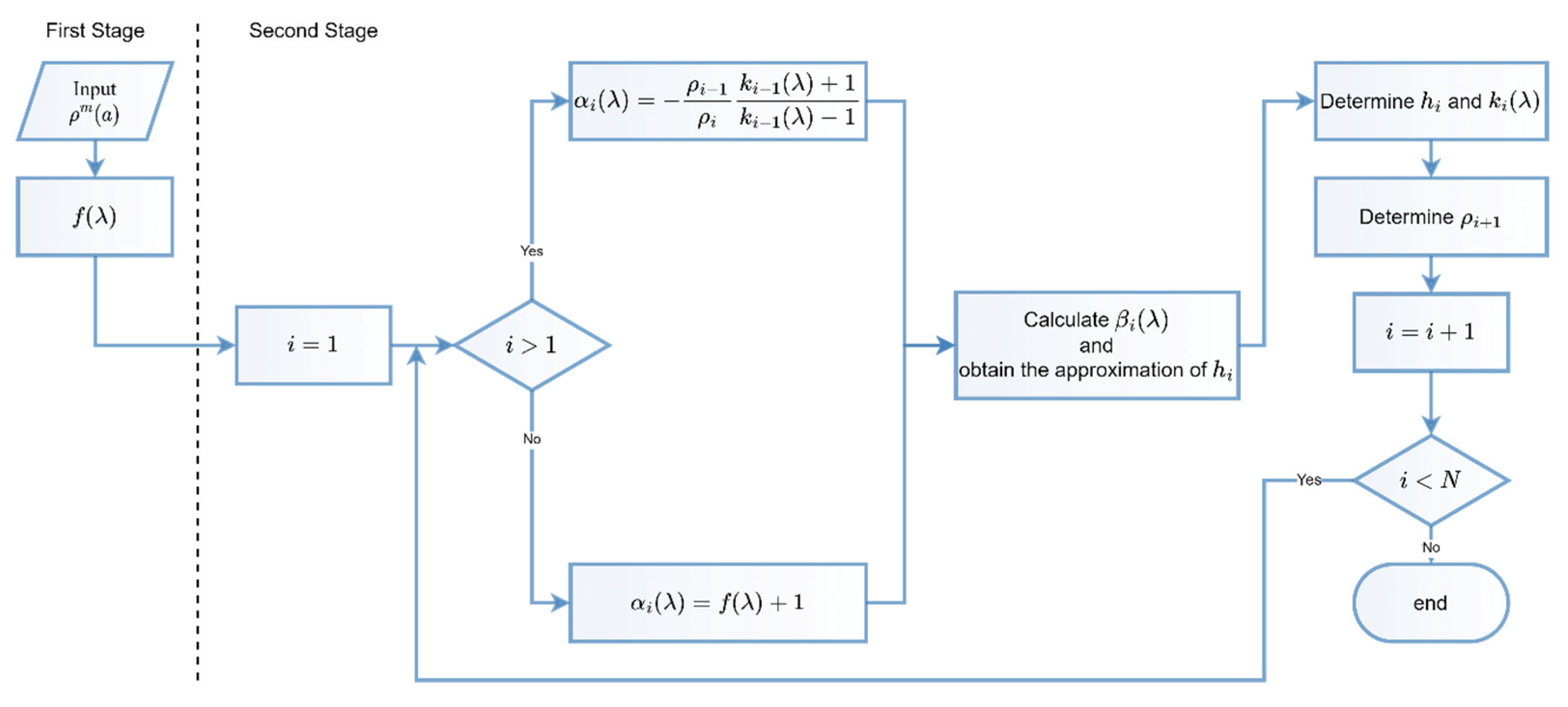
4. Inversion of Soil Parameters Using Kernel Function Characteristics

In this paper, we analyze the characteristics of the kernel function and introduce a method for inverting the soil resistivity (${\mathsf{\rho }}_i$) and depth ($h_i$) of each layer very simply using this characteristics. By analyzing the characteristics of $k_i$ and ${\mathsf{\alpha }}_i$ in the kernel function of (3), the parameters of the soil structure, that is, the soil resistivity and depth of each layer, can be obtained.

In general, the kernel function is a function used to theoretically calculate the apparent soil resistivity, as shown in (3). Additionally, from the parameters of the given land structure, the parameters of the deep layer are used in order, that is, $k_{n-1}\left(\mathsf{\lambda }\right)$, ${\mathsf{\alpha }}_{n-1}\left(\mathsf{\lambda }\right)$, $\cdots k_1\left(\mathsf{\lambda }\right)$, ${\mathsf{\alpha }}_1\left(\mathsf{\lambda }\right)$. When the parameters of the assumed soil structure approach the correct answer, the calculated value and the measured value of the apparent soil resistivity become closer. In other words, as the parameter of the soil structure approaches the correct answer, the kernel function also approaches the correct answer. However, the method proposed in this paper is a two-step method. In the first step, the kernel function is first obtained from the apparent soil resistivity. In the next step, we analyze the characteristics of the pre-acquired kernel functions to find ${\mathsf{\alpha }}_1\left(\mathsf{\lambda }\right)$, $k_1\left(\mathsf{\lambda }\right), \cdots , {\mathsf{\alpha }}_{n-1}\left(\mathsf{\lambda }\right)$,$k_{n-1}\left(\mathsf{\lambda }\right)$. Then, using the characteristics of ${\mathsf{\alpha }}_i\left(\mathsf{\lambda }\right)$ and $k_i\left(\mathsf{\lambda }\right)$, $h_i$ and ${\mathsf{\rho }}_{i+1}$ are subsequently obtained. Additionally, it is assumed that the soil resistivity of the surface layer can be known through a measurement of ${\mathsf{\rho }}_1$.

(1) Characteristics of k(λ): If $k_i\left(\mathsf{\lambda }\right)$ is known, ${\mathsf{\rho }}_{i+1}$ can be obtained if the soil resistivity, ${\mathsf{\rho }}_i$, is known.

In (3), as $\mathsf{\lambda }$ approaches infinity, then ${\mathsf{\alpha }}_{i+1}\left(\mathsf{\lambda }\right)$ converges to 1 as follows:

$$\underset{\lambda \to \infty }{\lim }{\alpha }_{i+1}\left(\mathsf{\lambda }\right)=\underset{\lambda \to \infty }{\lim }\left(1+\frac{2K_i{e}^{-2\mathsf{\lambda }{h}_i}}{1-K_i{e}^{-2\mathsf{\lambda }{h}_i}}\right)=1$$

(11)

Additionally, $k_i\left(\mathsf{\lambda }\right)$ converges to a constant as follows:

$$\underset{\lambda \to \infty }{\lim }{k}_i\left(\mathsf{\lambda }\right)=\underset{\lambda \to \infty }{\lim }\frac{{\mathsf{\rho }}_{i+1}{\mathsf{\alpha }}_{i+1}-{\mathsf{\rho }}_i}{{\mathsf{\rho }}_{i+1}{\mathsf{\alpha }}_{i+1}+{\mathsf{\rho }}_i}=\frac{{\mathsf{\rho }}_{i+1}-{\mathsf{\rho }}_i}{{\mathsf{\rho }}_{i+1}+{\mathsf{\rho }}_i}=k_i^c$$

(12)

Therefore, ${\mathsf{\rho }}_{i+1}$ can be obtained as follows from (12):

$${\mathsf{\rho }}_{i+1}\simeq \frac{1+k_i^c}{1-k_i^c}{\mathsf{\rho }}_i$$

(13)

For explanation, a four-layer soil structure was selected as shown in

Table 1. Soil parameters of a four-layer structure.

ith Layer	${\mathsf{\rho }}_{\mathit{i}} \left(\mathit{\Omega }m\right)$	${\mathit{h}}_{\mathit{i}} \left(m\right)$
1	235.32	1.2
2	3518.28	18.3
3	205.53	21.06
4	1504.71	∞

, and the parameters were also arbitrarily set.

Figure 2 shows the ${\mathsf{\alpha }}_i\left(\mathsf{\lambda }\right)$ and $k_i\left(\mathsf{\lambda }\right)$ corresponding to the soil parameters of the four-layer structure in Table 1. As mentioned in (11), Figure 2 shows that all ${\mathsf{\alpha }}_i\left(\mathsf{\lambda }\right)$ converge to 1 and $k_i\left(\mathsf{\lambda }\right)$ also converges.

As seen in (12), $k_i\left(\mathsf{\lambda }\right)$ converges to a constant which is the ratio of the soil resistivity of the adjacent layer. Therefore, if the convergence value of $k_i\left(\mathsf{\lambda }\right)$ is known, ${\mathsf{\rho }}_{i+1}$ can be obtained using the known soil resistivity, ${\mathsf{\rho }}_i$. As seen in Figure 3, if all the convergence values of $k_i\left(\mathsf{\lambda }\right)$ are known, all the soil resistivity, ${\mathsf{\rho }}_i,$ in Table 1 can be obtained.

(2) Characteristics of α(λ):

(i) Using the characteristics of ${\mathsf{\alpha }}_i\left(\mathsf{\lambda }\right)$, an approximate value of the depth, $h_i$, of each soil layer can be obtained.

In ${\mathsf{\alpha }}_i\left(\mathsf{\lambda }\right)$ in (3), $k_i\left(\mathsf{\lambda }\right)$ can be rearranged and expressed as follows:

$$k_i\left(\mathsf{\lambda }\right)=\frac{{\mathsf{\alpha }}_i\left(\mathsf{\lambda }\right)-1}{{\mathsf{\alpha }}_i\left(\mathsf{\lambda }\right)+1}{e}^{2\mathsf{\lambda }{h}_i}={\mathsf{\beta }}_i\left(\mathsf{\lambda }\right)e^{2\mathsf{\lambda }{h}_i},$$

(14)

where

$${\mathsf{\beta }}_i\left(\mathsf{\lambda }\right)=\frac{{\mathsf{\alpha }}_i\left(\mathsf{\lambda }\right)-1}{{\mathsf{\alpha }}_i\left(\mathsf{\lambda }\right)+1}$$

(15)

Since $k_i\left(\mathsf{\lambda }\right)$ tends towards a constant, $\frac{{\mathsf{\rho }}_{i+1}-{\mathsf{\rho }}_i}{{\mathsf{\rho }}_{i+1}+{\mathsf{\rho }}_i}$, as λ gets larger, ${\mathsf{\beta }}_i\left(\mathsf{\lambda }\right)$ also tends towards:

$${\mathsf{\beta }}_i\left(\mathsf{\lambda }\right)\simeq C_i{e}^{-2\mathsf{\lambda }{h}_i}$$

(16)

If we know the two coordinates in the graph of ${\mathsf{\beta }}_i\left(\mathsf{\lambda }\right)$, that is, ${\mathsf{\beta }}_i\left({\mathsf{\lambda }}_1\right)$, and ${\mathsf{\beta }}_i\left({\mathsf{\lambda }}_2\right)$ at ${\mathsf{\lambda }}_1$ and ${\mathsf{\lambda }}_2$, we can obtain the approximate value of $h_i$ using the following equation:

$$\frac{{\mathsf{\beta }}_i\left({\mathsf{\lambda }}_2\right)}{{\mathsf{\beta }}_i\left({\mathsf{\lambda }}_1\right)}=\frac{C_i{e}^{-2{\mathsf{\lambda }}_2{h}_i}}{C_i{e}^{-2{\mathsf{\lambda }}_1{h}_i}}=e^{-2h_i\left({\mathsf{\lambda }}_2-{\mathsf{\lambda }}_1\right)}$$

(17)

If (17) is rearranged for $h_i$, it follows:

$$h_i=-\frac{1}{2\left({\mathsf{\lambda }}_2-{\mathsf{\lambda }}_1\right)}\ln \frac{{\mathsf{\beta }}_i\left({\mathsf{\lambda }}_2\right)}{{\mathsf{\beta }}_i\left({\mathsf{\lambda }}_1\right)}$$

(18)

If ${\mathsf{\beta }}_1\left({\mathsf{\lambda }}_1\right)=0.34019$ and ${\mathsf{\beta }}_1\left({\mathsf{\lambda }}_2\right)=0.116488$ at ${\mathsf{\lambda }}_1=0.39$ and ${\mathsf{\lambda }}_2=0.84$ in Figure 4, the approximate value of $h_1$ can be obtained as follows:

$$h_1=-\frac{1}{2\left(0.84-0.39\right)}\ln \frac{0.11649}{0.34019}=1.19$$

(19)

(ii) Using the approximate value of $h_i$, a more precise $h_i$ and $k_i\left(\mathsf{\lambda }\right)$ can be estimated.

In (14), a simple program can obtain a more accurate $h_i$ than the approximate $h_i$ that tries to converge $k_i\left(\mathsf{\lambda }\right)$ to a constant. At the same time, $k_i\left(\mathsf{\lambda }\right)$ becomes more accurate the more accurate $h_i$ is.

As shown in Figure 5, $k_1\left(\mathsf{\lambda }\right)$ converges closer to a constant at $h_1=1.2$ m than at $h_1=1.19$ m. Therefore, determining the final $h_1$ to be 1.2 m is considered the correct decision. At the same time, the following $k_1\left(\mathsf{\lambda }\right)$ can be determined using (14).

$$k_1\left(\mathsf{\lambda }\right)=\frac{{\mathsf{\alpha }}_1\left(\mathsf{\lambda }\right)-1}{{\mathsf{\alpha }}_1\left(\mathsf{\lambda }\right)+1}{e}^{2.4\mathsf{\lambda }}$$

(20)

(3) The recursive properties of kernel functions:

All ${\mathsf{\alpha }}_i\left(\mathsf{\lambda }\right)$ and $k_i\left(\mathsf{\lambda }\right)$ can be obtained sequentially from the kernel function $f\left(\mathsf{\lambda }\right)$.

(i) Calculate ${\mathsf{\alpha }}_1\left(\mathsf{\lambda }\right)$ using $f\left(\mathsf{\lambda }\right)$.

${\mathsf{\alpha }}_1\left(\mathsf{\lambda }\right)$ is obtained as follows using (3):

$${\mathsf{\alpha }}_1\left(\mathsf{\lambda }\right)=f\left(\mathsf{\lambda }\right)+1$$

(21)

(ii) Obtain an approximation of $h_i$ using the characteristics of ${\mathsf{\alpha }}_i\left(\mathsf{\lambda }\right)$.

(iii) A more precise $h_i$ is obtained using the characteristics of converging to the constant $k_i\left(\mathsf{\lambda }\right)$. At the same time, $k_i\left(\mathsf{\lambda }\right)$ is determined.

(iv) ${\mathsf{\alpha }}_{i+1}\left(\mathsf{\lambda }\right)$ can be obtained using $k_i\left(\mathsf{\lambda }\right)$ as follows.

Reordering $k_i\left(\mathsf{\lambda }\right)$ in (3) with respect to ${\mathsf{\alpha }}_{i+1}\left(\mathsf{\lambda }\right)$ gives:

$${\mathsf{\alpha }}_{i+1}\left(\mathsf{\lambda }\right)=-\frac{{\mathsf{\rho }}_i}{{\mathsf{\rho }}_{i+1}}\frac{k_i\left(\mathsf{\lambda }\right)+1}{k_i\left(\mathsf{\lambda }\right)-1}$$

(22)

A flow chart for inverting the parameters of an $N$-layer soil structure is illustrated in Figure 6, where $f\left(\mathsf{\lambda }\right)$ is the estimated kernel function in the first step.

5. Numerical Examples

The case study is split into two. The first part shows the process of estimating the kernel function from the apparent soil resistivity using linearization. The second part shows the process of inversing the parameters by analyzing the characteristics of the kernel function.

5.1. Kernel Function Estimation Using Apparent Soil Resistivity

If the structure parameters of the soil are known, one can generate the apparent resistivity data for different electrode distances, a, using (2). Then, these generated data can be used to check the proposed analysis method. To verify that the linearization method is generally applicable to kernel function inversion, two different soil structures (two-layer and four-layer structures) are used.

5.1.1. Two-Layer Soil Structure

As shown in

Table 2. Parameters of the two-layer structure.

ith Layer	${\mathsf{\rho }}_{\mathit{i}} \left(\mathit{\Omega }m\right)$	${\mathit{h}}_{\mathit{i}} \left(m\right)$
1	132.9	5.1
2	20.4	∞

, a simple two-layer structure was arbitrarily selected. The 12 apparent soil resistivities in

Table 3. Apparent soil resistivity.

${\mathit{a}}_{\mathit{i}} ()$	${\mathsf{\rho }}_{\mathit{a}}^{\mathit{m}} \left(\mathit{\Omega }m\right)$	${\mathit{a}}_{\mathit{i}} \left(m\right)$	${\mathsf{\rho }}_{\mathit{a}}^{\mathit{m}} \left(\mathit{\Omega }m\right)$
0.1	132.9	15	32.6
0.5	132.8	20	25.3
1	132.4	30	21.8
3	122.8	40	21.0
7	79.3	50	20.8
10	53.6	60	20.7

were generated using (2) based on these parameters.

Therefore, the number of equations, ($M$), is 12. As can be seen in Figure 7a, the kernel function was well estimated by the proposed method. Additionally, it can be seen that the number of unknown b is the major factor. Through trial and error, it was confirmed that the kernel function, $f\left(\mathsf{\lambda }\right)$, can be accurately obtained only when $N\gg M$. Figure 7b shows the estimated kernel function according to the number of $N$. The kernel function is estimated properly when the number of $N$ is higher than a certain number. Figure 7a shows an estimate graph with $N=300$, which is in close agreement with the exact value.

5.1.2. Four-Layer Soil Structure

In

Table 4. Parameters of the four-layer soil structure.

ith Layer	${\mathsf{\rho }}_{\mathit{i}} \left(\mathit{\Omega }m\right)$	${\mathit{h}}_{\mathit{i}} \left(m\right)$
1	68	1.08
2	627.9	1.64
3	7.3	3.98
4	125.4	∞

, a four-layer structure was arbitrarily selected as an example of a complicated case. Based on the data in Table 4, 14 apparent soil resistivities in

Table 5. Apparent resistivity data.

${\mathit{a}}_{\mathit{i}} ()$	${\mathsf{\rho }}_{\mathit{a}}^{\mathit{m}} \left(\mathit{\Omega }m\right)$	${\mathit{a}}_{\mathit{i}} \left(m\right)$	${\mathsf{\rho }}_{\mathit{a}}^{\mathit{m}} \left(\mathit{\Omega }m\right)$
0.1	68.0	6	292.4
0.5	71.9	10	350.1
0.7	77.3	12	359.7
1.4	109.7	14	359.3
2.3	157.6	17	348.3
3.0	191.0	20	329.6
4	232.0	30	258.1

were generated using (2). Hence, $M=14$ and $N=300$. Again, the equation is the underdetermined system, and the unknown b was obtained by the QR decomposition method. Additionally, the approximation obtained in the same way closely matched the exact kernel function. Figure 8 shows the result.

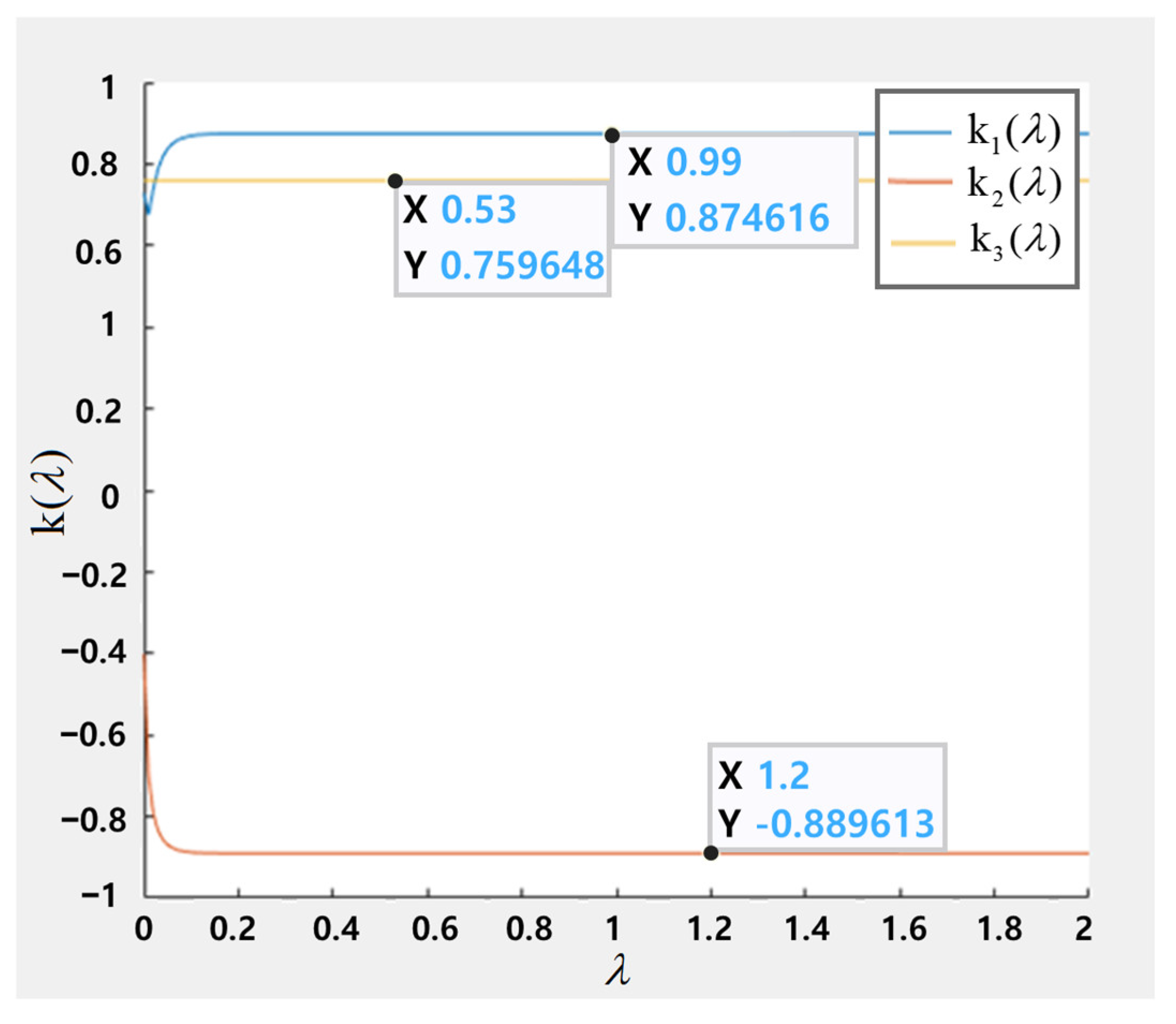
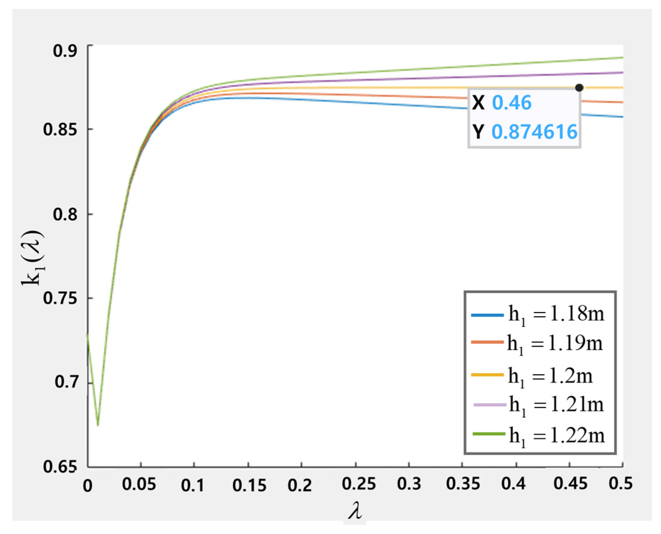
5.2. Inversion of Soil Parameter Using Kernel Function Characteristics

The four-layer soil structure in Table 4 was selected and the proposed method was verified using the kernel function estimated from the selected structure. The four-layer soil structure is represented by seven parameters: ${\mathsf{\rho }}_1$, ${\mathsf{\rho }}_2$, ${\mathsf{\rho }}_3$, ${\mathsf{\rho }}_4$, ${\mathrm{h}}_1$, ${\mathrm{h}}_2$, and ${\mathrm{h}}_3$. Here, ${\mathsf{\rho }}_1$ is assumed to be measurable. This is considered equal to the ground resistance of the earth’s surface. Therefore, we will demonstrate the procedure for finding six parameters as follows.

(1) Obtain ${\mathsf{\alpha }}_1\left(\mathsf{\lambda }\right)$.

Using the estimated kernel function, $f\left(\mathsf{\lambda }\right)$, as defined in (3), ${\mathsf{\alpha }}_1\left(\mathsf{\lambda }\right)$ is obtained as follows:

$${\mathsf{\alpha }}_1\left(\mathsf{\lambda }\right)=f\left(\mathsf{\lambda }\right)+1$$

(23)

(2) Calculate ${\mathsf{\beta }}_1\left(\mathsf{\lambda }\right)$ and find an approximation for $h_1$.

As defined in (15), ${\mathsf{\beta }}_1\left(\mathsf{\lambda }\right)$ is calculated as follows:

$${\mathsf{\beta }}_1\left(\mathsf{\lambda }\right)=\frac{{\mathsf{\alpha }}_1\left(\mathsf{\lambda }\right)-1}{{\mathsf{\alpha }}_1\left(\mathsf{\lambda }\right)+1}$$

(24)

The approximation of $h_1$ can be obtained using (18) as follows:

$$h_1=\frac{-1}{2\left({\mathsf{\lambda }}_1-{\mathsf{\lambda }}_2\right)}\ln \frac{{\mathsf{\beta }}_1\left({\mathsf{\lambda }}_1\right)}{{\mathsf{\beta }}_1\left({\mathsf{\lambda }}_2\right)}$$

(25)

Substituting the two coordinates (1.11, 0.0723) and (2.11, 0.0084) in Figure 9 into (25), an approximation of $h_1$ can be obtained as follows:

$$h_1\simeq \frac{-1}{2\left(1.11-2.11\right)}\ln \frac{0.0723}{0.0084}=1.074$$

(26)

(3) Determine $h_1$ and $k_1\left(\mathsf{\lambda }\right)$.

As shown in Figure 10, $k_1\left(\mathsf{\lambda }\right)$ converges closer to a constant at $h_1=1.08$ m than at $h_1=1.074$ m. Therefore, determining the final $h_1$ to be 1.08 m is considered to be the correct decision. At the same time, the following $k_1\left(\mathsf{\lambda }\right)$ can be determined using (14).

$$k_1\left(\mathsf{\lambda }\right)=\frac{{\mathsf{\alpha }}_1\left(\mathsf{\lambda }\right)-1}{{\mathsf{\alpha }}_1\left(\mathsf{\lambda }\right)+1}{e}^{2.16\mathsf{\lambda }}$$

(27)

(4) Obtain ${\mathsf{\rho }}_2$.

The second layer’s soil resistivity, ${\mathsf{\rho }}_2$, can be obtained using the characteristic that $k_1\left(\mathsf{\lambda }\right)$ converges to a constant as follows:

$$\underset{\mathsf{\lambda }\to \infty }{\lim }{k}_1\left(\mathsf{\lambda }\right)=k_1^c=\frac{{\mathsf{\rho }}_2-{\mathsf{\rho }}_1}{{\mathsf{\rho }}_2+{\mathsf{\rho }}_1}$$

(28)

Rearranging (28) with respect to ${\mathsf{\rho }}_2$, ${\mathsf{\rho }}_2$ can be obtained as follows:

$${\mathsf{\rho }}_2=\frac{1+k_1^c}{1-k_1^c}{\mathsf{\rho }}_1$$

(29)

In Table 5, using the apparent soil resistivity at the electrode span a = 0.1 m, ${\mathsf{\rho }}_2$ is calculated as follows:

$${\mathsf{\rho }}_2=\frac{1+k^{c_1}}{1-k^{c_1}}{\mathsf{\rho }}_1\simeq \frac{1+0.804567}{1-0.804567}\times 68=627.89$$

(30)

(5) Obtain ${\mathsf{\alpha }}_2\left(\mathsf{\lambda }\right)$.

Using (22) and ${\mathsf{\rho }}_1$, ${\mathsf{\rho }}_2$, and $k_1\left(\mathsf{\lambda }\right)$ which are obtained above, ${\mathsf{\alpha }}_2\left(\mathsf{\lambda }\right)$ can be obtained as follows:

$${\mathsf{\alpha }}_2\left(\mathsf{\lambda }\right)=-\frac{{\mathsf{\rho }}_1}{{\mathsf{\rho }}_2}\frac{k_1\left(\mathsf{\lambda }\right)+1}{k_1\left(\mathsf{\lambda }\right)-1}$$

(31)

(6) Calculate ${\mathsf{\beta }}_2\left(\mathsf{\lambda }\right)$ and find an approximation of $h_2$.

As defined in (15), ${\mathsf{\beta }}_2\left(\mathsf{\lambda }\right)$ is calculated as follows:

$${\mathsf{\beta }}_2\left(\mathsf{\lambda }\right)=\frac{{\mathsf{\alpha }}_2\left(\mathsf{\lambda }\right)-1}{{\mathsf{\alpha }}_2\left(\mathsf{\lambda }\right)+1}$$

(32)

The approximation of $h_2$ can be obtained using (18) as follows:

$$h_2=\frac{-1}{2\left({\mathsf{\lambda }}_1-{\mathsf{\lambda }}_2\right)}\ln \frac{{\mathsf{\beta }}_2\left({\mathsf{\lambda }}_1\right)}{{\mathsf{\beta }}_2\left({\mathsf{\lambda }}_2\right)}$$

(33)

Substituting the two coordinates (0.41, −0.25418) and (1.18, −0.02037) in Figure 11 into (33), an approximation of $h_2$ can be obtained as follows:

$$h_2\simeq \frac{-1}{2\left(0.41-1.18\right)}\ln \frac{-0.25418}{-0.02037}=1.6389$$

(34)

(7) Determine $h_2$ and $k_2\left(\mathsf{\lambda }\right)$.

As shown in Figure 12, $k_2\left(\mathsf{\lambda }\right)$ converges closer to a constant at $h_2=1.64$ m than at $h_2=1.6389$ m. Therefore, determining the final $h_2$ to be 1.64 m is considered the correct decision. At the same time, the following $k_2\left(\mathsf{\lambda }\right)$ can be determined using (14).

$$k_2\left(\mathsf{\lambda }\right)=\frac{{\mathsf{\alpha }}_2\left(\mathsf{\lambda }\right)-1}{{\mathsf{\alpha }}_2\left(\mathsf{\lambda }\right)+1}{e}^{3.28\mathsf{\lambda }}$$

(35)

(8) Obtain ${\mathsf{\rho }}_3$.

The soil resistivity, ${\mathsf{\rho }}_3$, of the third layer can be obtained as follows using the characteristic that $k_2\left(\mathsf{\lambda }\right)$ converges to a constant. That is, in the same way as for finding ${\mathsf{\rho }}_2$.

$${\mathsf{\rho }}_3=\frac{1+k_2^c}{1-k_2^c}{\mathsf{\rho }}_2$$

(36)

In Figure 12, it was found that $k_2\left(\mathsf{\lambda }\right)$ converged to −0.977015. Additionally, substituting the pre-obtained ${\mathsf{\rho }}_2=627.89 \Omega \mathrm{m}$ into the following equation, ${\mathsf{\rho }}_3$ can be calculated as:

$${\mathsf{\rho }}_3=\frac{1+k^{c_2}}{1-k^{c_2}}{\mathsf{\rho }}_2\simeq \frac{1-0977015}{1+0.977015}\times 627.89=7.299$$

(37)

(9) Obtain ${\mathsf{\alpha }}_3\left(\mathsf{\lambda }\right)$.

Using (22) and ${\mathsf{\rho }}_2$, ${\mathsf{\rho }}_3$, and $k_2\left(\mathsf{\lambda }\right)$ obtained above, ${\mathsf{\alpha }}_3\left(\mathsf{\lambda }\right)$ can be obtained as follows:

$${\mathsf{\alpha }}_3\left(\mathsf{\lambda }\right)=-\frac{{\mathsf{\rho }}_2}{{\mathsf{\rho }}_3}\frac{k_2\left(\mathsf{\lambda }\right)+1}{k_2\left(\mathsf{\lambda }\right)-1}$$

(38)

(10) Calculate ${\mathsf{\beta }}_3\left(\mathsf{\lambda }\right)$ and find an approximation for $h_3$.

As defined in (15), ${\mathsf{\beta }}_3\left(\mathsf{\lambda }\right)$ is calculated as follows:

$${\mathsf{\beta }}_3\left(\mathsf{\lambda }\right)=\frac{{\mathsf{\alpha }}_3\left(\mathsf{\lambda }\right)-1}{{\mathsf{\alpha }}_3\left(\mathsf{\lambda }\right)+1}$$

(39)

The approximation of $h_3$ can be obtained using (18) as follows:

$$h_3=\frac{-1}{2\left({\mathsf{\lambda }}_1-{\mathsf{\lambda }}_2\right)}\ln \frac{{\mathsf{\beta }}_3\left({\mathsf{\lambda }}_1\right)}{{\mathsf{\beta }}_3\left({\mathsf{\lambda }}_2\right)}$$

(40)

Substituting the two coordinates (0.18, 0.212384) and (0.43, 0.029032) in Figure 13 into (40), an approximation of $h_3$ can be obtained as follows:

$$h_3\simeq \frac{-1}{2\left(0.43-0.18\right)}\ln \frac{0.212384}{0.029032}=3.978$$

(41)

(11) Determine $h_3$ and $k_3\left(\mathsf{\lambda }\right)$.

As shown in Figure 14, $k_3\left(\mathsf{\lambda }\right)$ converges closer to a constant when $h_3=3.98$ m than with any other value of $h_3$. Therefore, determining the final $h_3$ to be 3.98 m is considered the correct decision. At the same time, the following $k_3\left(\mathsf{\lambda }\right)$ can be determined using (14).

$$k_3\left(\mathsf{\lambda }\right)=\frac{{\mathsf{\alpha }}_3\left(\mathsf{\lambda }\right)-1}{{\mathsf{\alpha }}_3\left(\mathsf{\lambda }\right)+1}{e}^{7.96\mathsf{\lambda }}$$

(42)

(12) Obtain ${\mathsf{\rho }}_4$.

The last layer’s soil resistivity, ${\mathsf{\rho }}_4$, can be obtained using the characteristic that $k_3\left(\mathsf{\lambda }\right)$ converges to a constant as follows:

$${\mathsf{\rho }}_4=\frac{1+k_3^c}{1-k_3^c}{\mathsf{\rho }}_3$$

(43)

Here, $k_3^c$ denotes the converged value of $k_3\left(\mathsf{\lambda }\right)$ with increasing $\mathsf{\lambda }$.

In Figure 14, it was found that $k_3\left(\mathsf{\lambda }\right)$ converged to 0.889978. Additionally, substituting the pre-obtained ${\mathsf{\rho }}_3=7.299 \Omega \mathrm{m}$ into the following equation, ${\mathsf{\rho }}_4$ can be obtained as follows:

$${\mathsf{\rho }}_4=\frac{1+k_3}{1-k_3}{\mathsf{\rho }}_3\simeq \frac{1+0.8895}{1-0.8895}\times 7.299=124.8$$

(44)

The estimated value is very close to the exact value.

6. Conclusions

In this paper, we propose a new method to efficiently invert the parameters of horizontal multilayer soil. Soil parameters can be inverted by analyzing the characteristics of the kernel function of the apparent resistivity integral equation. That is, all parameters are inverted sequentially in a single procedure in an analytical manner. The essence of the proposed method avoids the difficulties encountered in general optimization methods; namely, the calculation of the apparent resistivity and its derivative. A typical optimization method requires iteratively calculating the apparent resistivity and its derivative each time the parameters are updated to reduce the error function, which is computationally demanding. The numerical results show the feasibility and the key features of the proposed approach.

References

1. Karnas, G.; Maslowski, G.; Ziemba, R.; Wyderka, S. Influence of different multilayer soil models of grounding system resistance. In Proceedings of the International Conference on Lightning Protection (ICLP), Vienna, Austria, 2–7 September 2012. [Google Scholar]
2. Dawalibi, F.; Blattner, C.J. Earth resistivity measurement interpretation techniques. IEEE Trans. Power Appar. Syst. 1984, 103, 374–382. [Google Scholar] [CrossRef]
3. He, J.; Zeng, R.; Zhang, B. Methodology and Technology for Power System Grounding; John Wiley and Sons Ltd.: Singapore, 2013; pp. 86–89. [Google Scholar]
4. Lee, J.P.; Ji, P.S.; Lim, J.Y.; Kim, S.S.; Ozdemir, A.; Singh, C. Earth parameter and equivalent resistivity estimation using ANN. In Proceedings of the IEEE Power Engineering Society General Meeting, San Francisco, CA, USA, 16 June 2005. [Google Scholar]
5. Zhiqiang, H.; Bin, Z. Soil model’s inversion calculation based on genetic algorithm. In Proceedings of the 7th Asia-Pacific International Conference on Lightning, Chengdu, China, 1–4 November 2011. [Google Scholar]
6. Dan, Y.; Zhang, Z.; Yin, J.; Yang, J.; Deng, J. Parameters estimation of horizontal multilayer soils using a heuristic algorithm. Electr. Power Syst. Res. 2022, 203, 1206–1231. [Google Scholar] [CrossRef]
7. Zhang, B.; Cui, X.; Li, L.; He, J. Parameter estimation of horizontal multilayer earth by complex image method. IEEE Trans. Power Deliv. 2005, 20, 1394–1401. [Google Scholar] [CrossRef]
8. Pereira, W.R.; Soares, M.G.; Neto, L.M. Horizontal multilayer soil parameter estimation through differential evolution. IEEE Trans. Power Deliv. 2016, 31, 622–629. [Google Scholar] [CrossRef]
9. Zou, J.; Zhang, B.; Du, X.; Lee, J.; Ju, M. High-efficient evaluation of the lightning electromagnetic radiation over a horizontally multilayered conducting ground with a new complex integration path. IEEE Trans. Electromagn. Compat. 2014, 56, 659–667. [Google Scholar] [CrossRef]
10. Coelho, R.R.A.; Pereira, A.E.C.; Neto, L.M. A High-performance multilayer earth parameter estimation rooted in Chebyshev polynomials. IEEE Trans. Power Deliv. 2018, 33, 1054–1061. [Google Scholar] [CrossRef]
11. Yang, J.; Zou, J. Parameter estimation of a horizontally multilayered soil with a fast evaluation of the apparent resistivity and its derivatives. IEEE Access 2020, 8, 52652–52662. [Google Scholar] [CrossRef]
12. Seedher, H.R.; Arora, J.K. Estimation of two layer soil parameters using finite Wenner resistivity expressions. IEEE Trans. Power Deliv. 1992, 7, 1213–1217. [Google Scholar] [CrossRef]
13. Takahashi, T.; Kawase, T. Analysis of apparent resistivity in a multi-layer earth structure. IEEE Trans. Power Deliv. 1990, 5, 604–612. [Google Scholar] [CrossRef]
14. Zou, J.; He, J.L.; Zeng, R.; Sun, W.M.; Yu, G.; Chen, S.M. Two-stage algorithm for inverting structure parameters of the horizontal multilayer soil. IEEE Trans. Magn. 2004, 40, 1136–1139. [Google Scholar] [CrossRef]
15. Islam, T.; Chik, Z.; Mustafa, M.M.; Sanusi, H. Estimation of soil electrical properties in a multilayer earth model with boundary element formulation. Math. Probl. Eng. 2012, 2012, 472457. [Google Scholar] [CrossRef] [Green Version]
16. Ahmad, S.; Khan, T. Comparison of statistical inversion with iteratively regularized Gauss Newton method for image reconstruction in electrical impedance tomography. Appl. Math. Comput. 2019, 358, 436–448. [Google Scholar] [CrossRef]
17. Hohage, T.; Munk, A. Iteratively regularized Gauss–Newton method for nonlinear inverse problems with random noise. SIAM J. Numer. Anal. 2009, 47, 1827–1846. [Google Scholar]
18. Dan, Y.; Zhang, Z.; Zhao, H.; Li, Y.; Ye, H.; Deng, J. A novel segmented sampling numerical calculation method for grounding parameters in horizontally multilayered soil. Int. J. Electr. Power Energy Syst. 2021, 126, 126–135. [Google Scholar] [CrossRef]
19. Honarbakhsh, B.; Karami, H.; Sheshyekani, K. Direct characterization of grounding system wide-band input impedance. IEEE Trans. Electromagn. Compat. 2020, 63, 328–331. [Google Scholar] [CrossRef]
20. Chapra, S.C. Applied Numerical Methods with MATLAB for Engineers and Scientists, 2nd ed.; McGraw-Hill: New York, NY, USA, 2008; pp. 270–276. [Google Scholar]
Figure 1. Wenner configuration method and the multilayer soil structure.
Energies 16 02078 g001
Figure 2. α i ( λ )   and   k i ( λ ) by the parameters in Table 1.
Energies 16 02078 g002
Figure 3. k i ( λ ) by the parameters in Table 1.
Energies 16 02078 g003
Figure 4. β ( λ ) by the parameters in Table 1.
Energies 16 02078 g004
Figure 5. k 1 ( λ ) by the different h 1 in Table 1.
Energies 16 02078 g005
Figure 6. Flow chart for the inversion of soil parameters.
Energies 16 02078 g006
Figure 7. The estimated kernel functions using the data in Table 3.
Energies 16 02078 g007
Figure 8. The estimated kernel functions using the data in Table 5.
Energies 16 02078 g008
Figure 9. β 1 ( λ ) according to Equation (24).
Energies 16 02078 g009
Figure 10. k 1 ( λ ) according to the different h 1 .
Energies 16 02078 g010
Figure 11. β 2 ( λ ) according to Equation (32).
Energies 16 02078 g011
Figure 12. k 2 ( λ ) according to the different h 2 .
Energies 16 02078 g012
Figure 13. β 3 ( λ ) according to Equation (40).
Energies 16 02078 g013
Figure 14. k 3 ( λ ) according to the different h 3 .
Energies 16 02078 g014