Abstract
The use of photovoltaic systems has increased in recent years due to their decreasing costs and improved performance. However, these systems can be susceptible to faults that can reduce efficiency and energy yield. To prevent and reduce these problems, preventive or predictive maintenance and effective monitoring are necessary. PV health monitoring systems and automatic fault detection and diagnosis methods are critical for ensuring PV plants’ reliability, high-efficiency operation, and safety. This paper presents a new framework for developing fault detection in photovoltaic (PV) systems. The proposed approach uses machine learning algorithms to predict energy power production and detect anomalies in PV plants by comparing the predicted power from a model and the measured power from sensors. The framework utilizes historical data to train the prediction model, and live data is compared with predicted values to analyze residuals and detect abnormal scenarios. The proposed approach has been shown to accurately distinguish anomalies using constructed thresholding, either static or dynamic thresholds. The paper also reports experimental results using the Matthews correlation coefficient, a more reliable statistical rate for an imbalanced dataset. The proposed approach leads to a reasonable anomaly detection rate, with an MCC of 0.736 and a balanced ACC of 0.863.
1. Introduction
The decrease in the costs of photovoltaic (PV) systems, the trend of market prices, and the improvement in performance due to improved cell efficiencies and lower electrical conversion losses are why PV systems have become more frequently usd over the last decade. Furthermore, PV systems offer numerous benefits, including clean and safe energy generation, quiet operation, lower installation costs, ease of installation, and building integration [1,2]. As a result, the PV industries have seen significant growth in the fabrication of photovoltaic equipment and the number of installations. On the other hand, solar cell systems are susceptible to various faults in any system component (modules, cables, protective devices, transformers, and inverters), which can reduce their efficiency and energy yield [3]. This is mainly due to external operating conditions such as shadow effects, dirty modules, faulty inverters, variation in manufacturing, and module aging [4]. Furthermore, faults may cause increased fault effects or the creation of new faults. To avoid and reduce the occurrence and consequences of these problems, preventive or predictive maintenance is required [5]. Effective monitoring is required for implementing predictive maintenance. The system standards then emphasize the importance of outfitting PV projects with effective monitoring equipment and tools. This has been made feasible by the collaboration of numerous projects aimed at improving the technical qualities of PV plants, on the one hand, and developing more effective monitoring tools and systems, on the other.
PV health monitoring systems (PV-HMS) are critical for ensuring that the production output is managed and that any possible faults are identified [6]. Display operation, data monitoring, anti-theft, faults detection and correction, emergency stop, and misalignment loss minimization are all examples of monitoring systems [7]. In addition, high-efficiency monitoring allows the manufacturer or the owner to identify problems or the need to take action with solar panels. PV system fault monitoring has become increasingly crucial due to the often severe and dynamic climatic conditions and the growing structural complexity of the PV system. The faults are typically recognized and solved manually; however, this method is not recommended because it is time-consuming, imprecise, and potentially dangerous to the operator, especially in large-scale PV arrays. Instead, the automatic fault detection and diagnosis (FDD) methods are essential for system reliability, high-efficiency operation, and PV plant safety [3].
Machine learning (ML) is a powerful technology that enables systems to learn from data and improve their performance over time without explicit programming. As a subset of artificial intelligence, it uses algorithms and statistical models to recognize patterns, make predictions, and make decisions autonomously. In the field of fault detection, ML-based approaches are becoming increasingly popular as they can improve efficiency, accuracy, and reliability by analyzing large amounts of data and identifying patterns that may indicate a fault. Additionally, ML’s ability to handle high-dimensional, non-linear, missing, and uncertain data, provide early detection, and adapt to changing conditions make it an ideal technology for fault detection. The goal of using ML for fault detection include increased efficiency and speed, improved accuracy, reduced costs, adaptability, and early detection.
There are several methods for developing fault detection in photovoltaic systems, for example, using electrical measurements, environmental data, or images of PV panels. In this study, we are interested in the indirect method framework according to these three steps. The first step is to create a regression model with input from environmental data and output from electrical data. This step generates prediction data that can be compared to sensor measurement data. The second step is to produce residuals by comparing the predicted value from the first step’s model to the measured value from a sensor. This step has several evaluation metrics for comparing data. The final step is to produce the thresholds to determine abnormal data points. An anomaly detection algorithm could give an accurate model for estimating electricity production under normal operating conditions, which could then be used to detect anomalies. Power production samples that indicate significant discrepancies between those expected under particular operating conditions and measured power can be used to detect such abnormalities [8,9,10].
Jiang et al. [8] provide a complex fault detection and diagnosis methodology. The experiments in this work use simulation data and verify the effectiveness using simulation results. Mekki et al. [9] focus on fault detection under partial shade conditions. The estimated current and voltage comparison was used for the operating state of the considered photovoltaic module. They also analyze the relation between power production volume and the number of shading cells. We have conducted some experiments on our dataset, and have found that the hourly averages of the measurements, which is an idea of Massimiliano et al. [10], provide good accuracy because of the slow intrinsic dynamic of the solar signals. Massimiliano et al. [10] report results of proposed low complexity of the power production model archive anomaly detection, with a rate better than 90%. However, their report uses a true positive rate as accuracy, which not only provides the wrong perspective of the company but also refuses some significant false predictions. The main limitation of this work is that the authors use a single model for all data despite various irradiance and seasonality. In addition, the static threshold, which separates the abnormality of daily data, has been used in this work.
The following list summarizes the significant contributions of this paper:
- 1.
- We provide a framework for creating an indirect defect detection in photovoltaic systems. As the first step, we present the developed approaches from previous articles [8,9,10], which contain a variety of procedures and data, in order to identify faults and evaluate how well they function in our dataset, which was collected using data from Thailand;
- 2.
- The second step follows from the results of the first step. We choose the method that worked well and provided high accuracy using our data. Then, a configuration algorithm to create a regression model, which predicted the power output inside the best methodology, is provided;
- 3.
- Finally, the last step provides ideas for constructing residual thresholds, either static or dynamic thresholds. Each threshold is constructed for defining anomaly behavior by measuring residuals to achieve high accuracy and performance in detecting abnormal scenarios. In this step, we compare one static and three dynamic threshold methods, such as daily threshold using Prophet, which is a time series forecasting and calculates the trend of residuals. The monthly threshold, which creates a constant threshold reliant on the month, has been constructed by ANN. Lastly, an hourly threshold was created by computing the threshold of each hour and summarizing the anomaly behavior of each day.
Our workflow differs from other publications by presenting the experimental results of various machine learning models to determine the most effective approach for predicting energy production. Furthermore, while previous research has focused on static thresholds for detecting abnormalities, we introduce a dynamic threshold approach that significantly improves the efficiency of automatic fault detection. Additionally, we address the common issue of imbalanced datasets in fault detection by utilizing the Matthews correlation coefficient as a more reliable statistical measure rather than solely relying on accuracy scores.
The rest of this paper is structured as follows: Section 2 reports a summary of the main literature in the related method. Section 3 provides a machine-learning model used in our experiment. Section 4 enters the methodology part, including anomaly detection and evaluation technique. This part provides all the details about the related ideas, including existing work and our ideas. The details of the data are described in Section 5, and data preprocessing is also illustrated in this section. Section 6 provides the results, including experimental pre-existing ideas, comparing machine learning models, and comparing static threshold and proposed dynamic thresholds for anomaly detection. Finally, Section 7 concludes the paper.
2. Related Work and Background
The rapid growth of photovoltaic (PV) technology and the growing number and size of PV power plants need increasingly sophisticated and intelligent health monitoring systems to maintain the dependable operation and high energy availability. For example, in Ref. [11], the authors discuss the various techniques: Artificial neural network (ANN), fuzzy logic, decision tree, support vector machine (SVM), k-nearest neighbors(KNN), and more, and also different kinds of data, such as electrical or environmental measurements and images of PV panels, which are commonly used. All the applications differ in various aspects, e.g., input data, data preprocessing, model type, and structure of prediction methodology. They describe the application of artificial neural networks for PV fault detection, diagnosis, and analysis from many aspects. The reported classification archive success rate is higher than 90%, which is proof that AI deserves to be explored for health monitoring in a photovoltaic system. In Ref. [12], the authors assessed the effectiveness of various machine learning techniques and used them to look for abnormalities in photovoltaic components.
The concept of the indirect method, previously cited, is the idea of fault detection diagnosed by comparing the predicted power from the model and measured power from a sensor. The methodology to figure out a good model, matrices to create residuals, and thresholding idea is the biggest challenge for this concept. However, there are a few papers discussing this idea. For photovoltaic fault detection and diagnosis, which use the indirect method concept, Ref. [11] provides different techniques that explain their ideas. By merging ANN and analytical approaches, the author suggested a strategy for string-based PV systems in Ref. [8]. Based on the measured irradiance and module temperature, a multilayer feed-forward ANN is utilized to forecast the power. The expected power generated by the ANN is then compared to the actual power measured by the PV system in the diagnosis section. The analytical method is used to determine the cause of the fault based on the power difference. Ref. [9] presents an ANN-based method for detecting faulty states of PV modules online under partially shaded conditions. It enables real-time fault detection by estimating the monitored system’s electrical outputs (output current and voltage) using only two meteorological parameters (solar irradiance and cell temperature). It could also detect possible anomalies in the PV module through real-time correlation of estimated and measured performance under variable conditions. Ref. [10] describes a method for detecting irregularities in PV systems and issuing maintenance notices in advance. The AC power production prediction model is based on an Artificial Neural Network (ANN), which can estimate AC power generation using solar irradiation and PV panel temperature measurements. Live PV system trend data is then compared to the model’s output, and the residuals vector is evaluated to discover anomalies and create daily predictive maintenance notifications.
We recognize that the related works in the literature examine the model development phase, either using regression models or detection techniques, with the goal of identifying anomalies. Nevertheless, none of them compare a different model used to predict power output and experiment with other ideas.
3. Machine Learning Models
In this section, we provide a brief taxonomy of the learning paradigms, aiming to provide some perspective on the content of this paper. Learning in the context of machine learning (ML) is the process of converting available input or training data (experience) into output (knowledge or expertise); consequently, machine learning is an interaction between the learner and the environment. Supervised learning is a task of interaction in which the environment is the teacher that supervises the learner by providing extra information (label). For example, the learner receives training e-mails that provide the label spam/not-spam, and thus a successful learner should be able to check/predict whether a set of words whose appearance in an unseen e-mail is spam or not. Models are a representation of actual or natural phenomena in the form of mathematical equations, e.g., a linear function that consumes information involving current power consumption in households to predict next-hour energy used volume.
Methods are an approach to problem-solving. In machine learning, a method is an approach that finds the parameters of a model using the given training data, e.g., gradient methods of optimization are used in training ML models. Algorithms are a set of instructions, sometimes written in pseudo-code, that exhibit the exact operations that need to be done to create an implementation of a given method.
Finally, implementations are a piece of code realized on some algorithms. In this work, we used the implementation of machine learning algorithms: Scikit-learn, a Python module integrating a wide range of machine learning algorithms for medium-scale supervised and unsupervised problems [13]. Additionally, for deep learning algorithms, we used Tensorflow [14] and Keras [15].
3.1. Linear Models
One of the most basic statistical tools for modeling is linear regression, which performs the relationship model between some explanatory variables and some real-valued outcome. Let X be an input space subset of and Y a measurable subset of , we would like to learn a linear function that best estimates the relationship between variables (i.e., when and ).
However, when the independent input variables are highly correlated, simple regression may be unstable [16]. Then, thus the Ridge regression or Linear least squares with regularization was introduced to carry out stable estimates of the coefficients by adding a regularization term for reducing the effects of the correlation.
To produce interpretable models but also show the stability of estimates such as Ridge regression, the Lasso (least absolute shrinkage and selection operator) regression was proposed [17]. Instead of using regularization, the Lasso model uses -norm for shrinking some variables and setting some to 0. The regularization term in Lasso shrinks some coefficients and sets others to 0, hence it performs feature selection to retain good features that exhibit relatively stronger effects on predictions. Moreover, shrinking coefficients tend to make the model more stable, such as Ridge regression; that is, the learner not only provides interpretable models but also stable models.
When the number of independent variables is much bigger than the number of data in the training set, the Lasso model is not a very satisfactory features selection method [18]. To improve the accuracy and interpretation of the model and overcome some limitations in the Lasso model, the Elastic-Net regression, a regularization technique, was introduced. By continuing shrinkage and simultaneously selecting variables, instead of adding either or regularization, the Elastic-Net model has both and regularization terms.
Stochastic Gradient Descent (SGD) [19] is an iterative algorithm that optimizes an objective function. In gradient descent we used the ’true’ gradient of the empirical risk; however, in SGD, the gradient is approximated by choosing a random sample in the training set. One advantage of this manner is that the computational cost at every iteration is low when the training set is huge, hence it is remarkably effective in large-scale machine learning tasks. More importantly, when using convex loss function, the SGD will converge to a global optimum, otherwise, it converges to a local minimum [20].
3.2. Kernel Methods
One of most widely used machine learning, kernel methods are flexible techniques that can be used to extend algorithms to define non-linear prediction. Unlike linear methods, kernel methods are replacing the original data in the input space with “kernels” or “kernel functions”, which extend algorithms (e.g., Support vector machines) to a linear separation in a high-dimensional space, or (equivalently to) a non-linear separation in the input space. For any constant , , and for all in the input space ; basic kernel functions are defined as the following,
Support vector machines (SVMs) [21] are supervised learning models associated with machine learning algorithms that receive and analyze data for building classification or regression models. The main idea behind SVMs was mapping non-linear input vectors to a high-dimensional space by using kernels, then in that space a linear decision model is constructed. Support vector regressions (SVRs) [22] are regression techniques based on the concept of SVMs. SVRs are an extended soft-margin SVMs that instead of using the hinge loss function, use -insensitive loss to make robust and sparse models [23].
3.3. Ensemble Models
Ensemble models are a combination of several models of predictions for improving the generalization performance and robustness over a single estimator [24,25,26], and consist of averaging and boosting methods. In averaging methods such as Bagging [27] or Random forests [28], the approach builds several models and averages their predicted values as the output from an ensemble model. On the other hand, in boosting methods, e.g., AdaBoost [29] or Gradient Tree Boosting [30], the approach sequentially builds estimators and tries to reduce the bias of the combined model. In this work we used Random forests (an averaging approach), Gradient Boosted Decision Trees (a boosting approach), and Adaptive Boosting (a boosting approach) for building models.
The core concept of the Random forests method is to combine the decision tree predictors that each tree depends on, such as the values of independent and identically distributed random sample vectors. This idea is not only applicable to classification but also regression problems. Random forests are one of the effective tools used for prediction; according to the law of large numbers, they do not overfit and give results that are competitive with boosting methods.
The goal of boosting methods is to fit a sequence of weak learners (learners whose performance is slightly better than random guessing), which converges to a strong learner.
The similarity between the boosting and averaging method is the use of an ensemble of predictors. In contrast, the averaging approach tries to fit its predictions to bootstrapped data; in the boosting method, each learner uses information from previous learners (sequentially learning). Gradient Tree Boosting involves mimicking a gradient descent algorithm in sense of updating learners by their negative gradient and its final prediction is an average of all the weak learners. On the other hand, AdaBoost’s final prediction is a weighted average and its updating step depends on modified weights rather than the gradient of loss functions.
3.4. Neural Network Models
Neural network or artificial neural networks (ANNs) are inspired by the structure of neural networks in the brain. They are a model of computation, which consists of a number of computing nodes or so-called neurons that are connected to each other in a complex network [31]. In this article, we focused on feed-forward neural networks, which are a form of supervised learning that use hierarchical layers to represent high-dimensional non-linear models.
The concept of feed-forward neural networks is to approximate function that best fits the training set T, which is the same as in linear regression methods. Instead of directly mapping the training points to the outcome predictions, feed-forward ANNs involve mapping data of the input layer to the hidden layers and thus mapping values in the last hidden layer to the output layer to perform predictions. There can be one or more non-linear layers in-between the input and the output layer. This paradigm is the so-called Multi-layer Perceptron (MLP). Optimization algorithms or optimizers are algorithms that solve the optimization of objective functions in ANNs. Normally, ANNs can be gradient descending or stochastic gradient descending in cases of large-scale learning. In this work we used Adam [32], which is an algorithm used for stochastic optimization. It requires little memory and is computationally efficient.
4. Methodology
As previously discussed, this work aims to enhance the efficiency of automatic fault detection through an indirect method. We have divided this section into three main parts. The first part, Anomaly, delves into previous research that utilizes an indirect approach for implementing a fault detection algorithm. Through careful examination, we determine an appropriate approach that involves data frequency and residual types that align with our data. We conduct experiments using various machine learning techniques to ensure that we achieve an optimal prediction model. Our investigation revealed that previous research only employed static thresholds to identify abnormalities. To boost the efficiency of fault detection, we introduce three dynamic thresholds that differentiate normal behavior from abnormal scenarios, taking into consideration time factors such as monthly, daily, and hourly. The last part of this section is dedicated to evaluation techniques, where we introduce the Matthews correlation coefficient as a more reliable statistical measure for evaluating the detection performance of our model. This approach is particularly suitable for imbalanced datasets such as the ones encountered in fault detection problems.
4.1. Anomaly Detection
In this section, we will introduce our process to create anomaly detection. However, some steps have been modified as a result of our data being labeled abnormal on a daily basis. Jiang et al. [8] provided a step that starts with a build regression of minutely collected data by ANN using Solar Irradiance and Module Temperature as the input and power output as the output. Then, they compute the residuals from the relative error between the predicted power and measured power . The threshold idea of this paper is a static threshold, which is defined as constant. The process given in Ref. [8] is sketched in Figure 1. We determined the threshold for this experiment to be through a process of trial and error. Consequently, we obtained the predicted behavior of each minute point in data. The day is labeled as normal if there are more typical than abnormal states. On the other hand, the day is labeled as an abnormal state if there is a normal state less than an abnormal one.
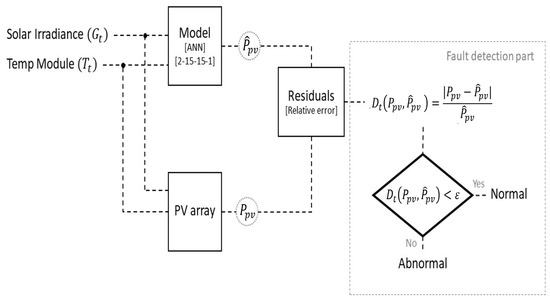
Figure 1.
Anomaly detection process. Developed from Ref. [8].
Mekki et al. [9] considered on ANN in order to estimate the two outputs photovoltaic current and voltage . Each output has its own residuals and , respectively, which are given by
where are the measured values of the output photovoltaic current produced in A and voltage in V, respectively, are the estimated values of the output photovoltaic current produced in A and voltage in V, respectively, by the developed ANN-based model. In addition, and have their own pre-defined threshold and , respectively. The grid parameters of and have been set as shown in Table 1. In the proposed method, the residual has the threshold and the residual has the threshold . If the residual errors and exceed the given threshold values , the PV module’s operational state will be contrasted with its faulty state (abnormality). The process given in Ref. [9] is sketched in Figure 2.

Table 1.
Grid parameters setting of in our experiment. Developed from Ref. [9].
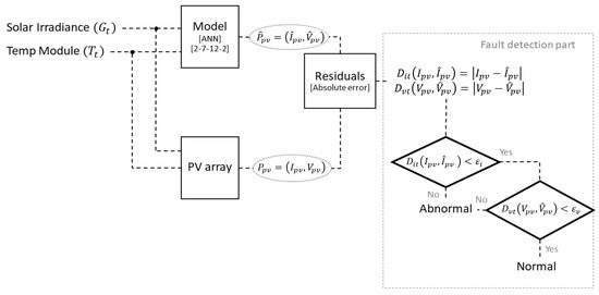
Figure 2.
Anomaly detection process. Developed from Ref. [9].
Recently, Massimiliano et al. [10] built the regression of hourly data by ANN using power output (Ppv) as the output. They introduced the two daily level thresholds as the following:
where is the RMSE computed during the ANN validation and K is an appropriate number of peak sun hours (in Ref. [10], ) Figure 3. They compute hourly residuals from absolute error between prediction and measure value . After that, daily residuals will be calculated from the summation of hourly residuals on the same day. This paper uses peak sun hours at . If the daily residuals are above the thresholds, they are labeled as abnormal.
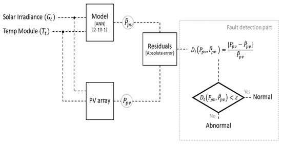
Figure 3.
Anomaly detection process. Developed from Ref. [10].
4.2. Residual Analysis
In the previous section, we introduced a method to create a prediction model and obtain the residuals. All the above methods use residuals, calculated by comparing the predicted and measured values for separate abnormalities of data points. However, after some experiments, we investigated that the static threshold did not have that much ability to capture the abnormality of a data point. We noticed some relations inside data between residuals and time, not only time, which means a date or sequence of date, but also a time in each day. Consequently, we would like to remove the weakness of the static threshold by proposing three novel approaches for the analysis of the residuals to determine the abnormality of data.
By only focusing on the residuals analysis, we have proposed three novel approaches according to these three concepts: time series using Prophet, ANN using month character, and hour vote. These three concepts have been described below.
4.2.1. Daily Threshold Using Prophet
The Facebook data scientist team created an open-source forecasting framework known as FbProphet. It is utilized to forecast time series data using an additive model, making forecasting more approachable and straightforward. It functions best when there are multiple seasons of historical data and time series with substantial seasonal effects [33]. Prophet employs regressive models such as ARIMA, exponential, and other models that are comparable. According to our assumption, the residual signal is the time series intended to be forecasted using Prophet [33] in Python. The concept is to forecast the values of the next four months using past time series information. Additionally, the Prophet is built on this equation’s combination of decomposable time series.
There are three main components in Equation (4), where a trend function called g(t) is used to represent and fit non-periodic changes in time series, such as piecewise linear growth or logical growth. A holiday term, h(t), reflects the influence of erratic holiday effects that may occur over one or more days. S(t) is a periodic term representing the periodic change (for example, the seasonality of each year). is an error representing unusual model modifications and is thought to follow a normal distribution.
The amount of change points (n-changepoints) in the dataset is a critical Facebook-Prophet parameter. Here, 25 is usually the value. Change points are evenly distributed on the first 80% of the time-series signal. The changepoint prior scale reveals how adaptable the change points can be or how much they can accommodate the data. It usually has a value of 0.05. The seasonality mode option defines the multiplicative and additive modes. The forecast trend and the seasonality’s impact are combined because the default mode is additive. The Prophet parameters grid is displayed in Table 2 with 162 potential models.
Table 2.
Grid parameters of Prophet. From Ref. [12].
We used the first substation, which has less abnormal data, to create a prediction model in the experiment. The second substation contains a lot of abnormal data to evaluate fault detection. Nonetheless, we constructed the residual prediction model using Prophet in the first substation data and analyzed it on the second substation. Figure 4 represents the workflow used in this idea. According to the first substation containing less abnormal data, we noticed that residuals would have less value. On the other hand, residuals in the second substation have a high value due to the dataset containing massive abnormal data. Furthermore, thresholds have to adapt, causing different natures of data too. The threshold has been computed as described in Equation (5).
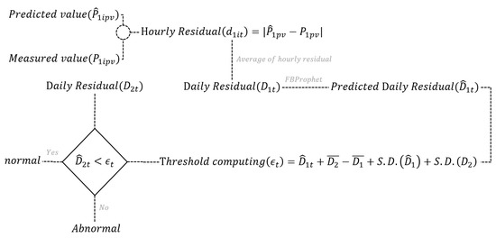
Figure 4.
Process chart of analyzing the residuals using the Prophet threshold.
4.2.2. Monthly Threshold Using ANN
This second approach still contains some concepts of the previous approach, which believes that time affects the residual. Based on engineering knowledge, seasonality affects the photovoltaic systems due to the sun’s movement and the temperature character. Consequently, we have proposed thresholds depending on the month of a data record. The model to create a threshold has been constructed following Figure 5.
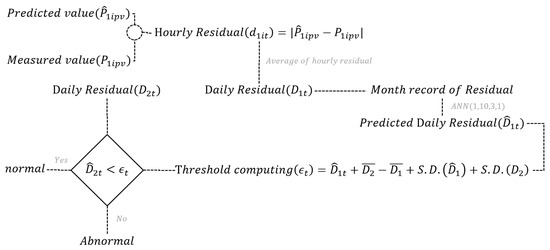
Figure 5.
Process chart of analyzing the residuals using the month threshold.
The residuals prediction model has been constructed using the month as input and residuals as output. The architecture of the ANN model has been designed using four layers with nodes , and 1, respectively. The mean square error has been used as loss and Adam as the optimizer. As mentioned in the Prophet part, there are differences between the first and second substations. Consequently, the threshold used is config, similar to the Prophet threshold.
Following these steps, we obtained a model that tries to predict the residuals of daily data. This model has led us to construct an adaptive threshold that depends on a month by computing the threshold, as shown in Figure 5.
4.2.3. Hourly Threshold Using 95th Residual’s Percentile
The final approach is constructed using the idea that each hour in a day produces a different amount of energy. We figure out the residual from each hour by separating the abnormality of the hourly data point. However, we are interested in the abnormality of daily data, so the details of this approach are described in Figure 6.
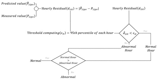
Figure 6.
Process chart of analyzing the residuals using the hour vote threshold.
There are a few abnormalities in the first substation, which we concluded as being due to most of the hourly data being standardized. Then, we set the residual threshold of each hour at the 95th percentile. The production ability of the first and second substations is similar; the difference between the two substations is that the first substation contains normal energy production behavior while the second substation contains abnormal behavior on some days. The same identicals of both substations in part of energy production efficiency are the reason why this threshold is not configured. Then, the 95th percentile of each hour in the first substation should be able to separate the outlier data that appear in each hour of the second substation.
4.3. Evaluation Technique
The model was created with the objective of predicting the power output from a solar panel. Overfitting will therefore be a value of concern. An overfitting problem is a modeling error occurring when a function is too closely aligned to the initial dataset. Consequently, the model cannot generalize well enough to predict unseen data. Cross-validation has been used to solve overfitting. It tests the effectiveness of machine learning models, and it is also a re-sampling procedure used to evaluate a model if we have limited data. The k-fold cv is the method used to divide the data into k equal parts to create and test the model, then compute the mean of model performance and use the model to predict the test set.
There are several techniques used to create anomaly detection. Consequently, many evaluation matrices would be called to create the regression predicting power output or producing the residuals determining abnormality. Given that is the observed power output value from sensor and is the predicted power output from the model where . The Root Mean Square Error (RMSE), which can be used for the loss function of the regression model, is the standard deviation of the residuals (prediction errors), calculated as Equation (6).
In this paper, we use the Matthews correlation coefficient to evaluate the detection performance of the model. Matthews correlation coefficient (MCC) is a more reliable statistical rate that produces a high score only if the prediction obtained good results in all of the four confusion matrix categories, true positives (TP), false negatives (FN), true negatives (TN), and false positives (FP), calculated as Equation (7)
5. Data Description
The data used in this study was collected from a solar power plant located in Phichit, Thailand. The sensor data was collected between January 2014 and May 2019 and includes detailed information on the power output from the photovoltaics system and environmental factors. Each data point includes a timestamp, solar irradiance, module temperature, and power output from the solar panel which are described in Table 3. In our experiment, we focused on two substations. The first substation’s data was collected from January 2014 to May 2019, but some data was missing due to sensor issues. After preprocessing, the data contains 478,713 rows and 888 days, 14 labeled as abnormal days. The second substation’s data was collected between June 2015 and June 2017 and contained 271,634 rows and 504 days, 102 labeled as abnormal days after preprocessing. The first substation’s data was used to create a regression model and thresholds. In contrast, the second substation’s data was used to test the model’s performance and ability to detect abnormal days. This approach was chosen as both substations use the same solar irradiance sensor and have similar energy production behavior, as we will discuss later in the study. However, the first substation contains fewer abnormal days than the second, making it more suitable for creating an energy production prediction model. On the other hand, the second substation, with more abnormal days, is better suited for evaluating fault detection.
Table 3.
Feature descriptions.
Regarding data preprocessing, we select data from 8 a.m. to 5 p.m. daily, as this time is suitable for the photovoltaic system. Following that, we eliminate unusual data by selecting only data with solar irradiance between 0 and 1260, with 1260 calculated from the 99th percentile of solar irradiance value. Furthermore, we select only data with temperature module values greater than 0 due to data occurring with some negative values that do not correspond to the actual environment. All the steps mentioned before are preprocessing steps in minute data, which provides hourly data in the next step. Hourly data were generated by averaging data minutely in the same hours. Furthermore, because minutely data did not record the entire minute in hours, we selected only hours with more than or equal to 54 min in minutely data. These hourly data will be used to build a regression model that will predict the amount of power generated by the solar panel based on solar irradiance and temperature module value.
Figure 7 and Figure 8 display the correlation matrix, which illustrates the correlation coefficients among the key elements of the first and second substations. The matrix calculates the linear correlation between the variables, where 1 indicates a strong positive correlation and −1 indicates a strong negative correlation. From the matrix, we can identify relationships between each feature that motivated us to include them in the model’s input. Furthermore, this confirms that it is possible to use the energy production prediction model trained on the first substation’s data on the second substation, as they have similar relationships between variables. To show an example of the relation between power output, solar irradiance, and module temperature, these strong relations have been examined in Figure 9, Figure 10 and Figure 11.
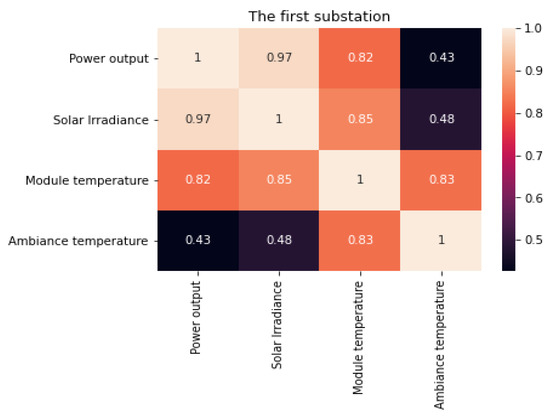
Figure 7.
Correlation matrix among each feature for the first substation.
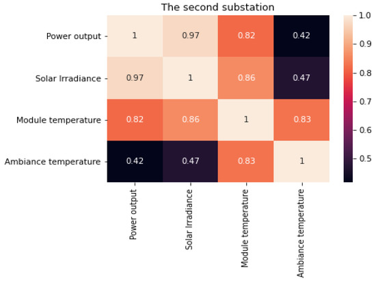
Figure 8.
Correlation matrix among each feature for the second substation.
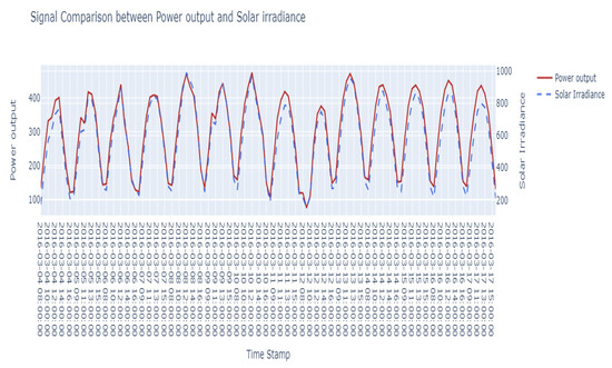
Figure 9.
Signal comparison between power output and solar irradiance of the first substation.
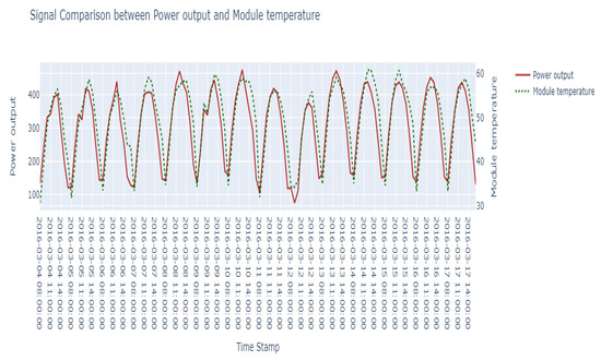
Figure 10.
Signal comparison between power output and module temperature of the first substation.

Figure 11.
Signal comparison between solar irradiance and module temperature of the first substation.
6. Results and Discussion
This section presents the results and discussion of the experimentation based on the methodology outlined in the previous section. We first applied pre-existing approaches from the literature [8,9,10] to our preprocessed data to determine suitable data frequency and residual types. We then used this information to select the most appropriate machine learning techniques through experimentation. Finally, we proposed and tested three dynamic thresholds using the suitable data frequency, residual types, and energy production prediction model obtained from the previous steps. Together, these steps provide a comprehensive approach for conducting fault detection in photovoltaic systems, which is the primary objective of this work.
6.1. Experiments Using Pre-Existing Ideas
We present the results of applying the pre-existing methods discussed earlier. Jiang et al. [8] and Mekki et al. [9] set their thresholds by selecting a constant value suited to their data. According to this fact, we decided to consider residual variation before determining the pre-defined threshold that would provide good efficiency through a trial-and-error process. Figure 12 illustrates the grid search to find the optimal values of and , and the results were evaluated using MCC and ACC scores. Consequently, we defined the Mekki et al. [9] thresholds as follows: the Upv’s residuals threshold at 300 and the Ipv’s residuals threshold at 70. On the other hand, we set the threshold of Jiang et al. [8] at 0.08. Note that the result of Massimiliano et al. [10], presented in Table 4, used lower or second-level thresholds due to their efficiency, which we will be discussed further.
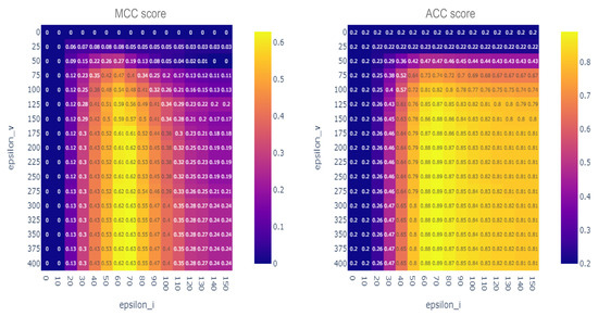
Figure 12.
Grid-search of and using the MCC and ACC score.
Table 4.
Detection scores of the pre-existing workflow. Developed from Refs. [8,9,10].
Table 4 shows the experimentation result using pre-existing approaches in our dataset. As a result, the existing approaches [8,9,10] each have their strengths and weaknesses. Jiang et al. [8] had the highest true positive rate but the worst false positive rate, resulting in the lowest detection rate. On the other hand, Mekki et al. [9] had the best false positive rate but the lowest true positive rate. Massimiliano et al. [10] provided a balanced outcome reflected in the MCC value and confusion matrix. According to this experimentation, the configuration of an algorithm that creates a regression model to predict power output using the approach of Massimiliano et al. [10] was further examined in the following step.
6.2. Compare Machine Learning Algorithms for Photovoltaic Models
As previously discussed, the approach of Massimiliano et al. [10] was found to be the most suitable for our dataset. Based on our experimentation, we determined that the optimal data frequency is hourly data, as it captures the slow intrinsic dynamic of the solar signals. Furthermore, we found that using absolute error as a residual computation method is suitable for our dataset. We experimented with machine learning techniques to determine the best approach for distinguishing abnormalities from normal behavior. As outlined in Section 4, the threshold in Massimiliano et al. [10] was defined with two levels computed from the RMSE between the predicted and measured values. The first level was calculated from RMSE * peak sun hours *3, while the second was calculated from RMSE * peak sun hours *5. We also provided a detection score for each regression model based on each ML technique. However, it is important to note that this work does not provide a prediction score, such as the Root mean square error or the coefficient of determination for each machine learning technique, as it is not the main objective of the work.
Table 5 and Table 6 demonstrate that the MLP regressor model is an excellent choice for building a regression model that predicts power output and is compatible with the approach of Massimiliano et al. [10]. This technique achieved high MCC scores of 0.638 and ACC of 0.843 in the first-level thresholds. This result also supports Massimiliano et al. [10] because the prediction model in their work uses a single layer with 10 nodes of an Artificial Neural Network, which is similar to an MLP regressor. It is worth noting that both thresholds have different strengths and weaknesses as the first-level threshold has a high true positive rate but also has a high false positive rate; on the other hand, the second-level threshold has a low false positive rate but contains a high false negative rate, as seen in Figure 13.
Table 5.
Detection score of each regression model in the first level threshold.
Table 6.
Detection score of each regression model in the second level threshold.
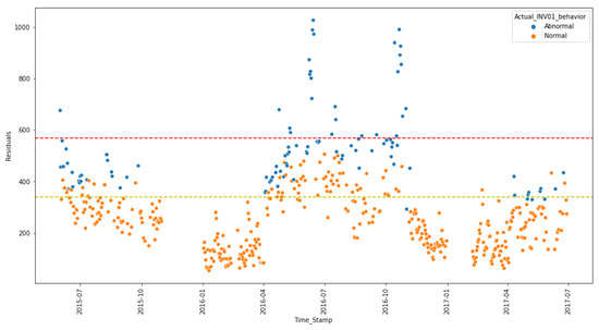
Figure 13.
Anomaly detection using the threshold. Developed from Ref. [10].
6.3. Comparing the Proposed Method to Create Dynamic Threshold for Anomalies Detection
Figure 13 shows that the first level is capable of collecting abnormal states without mixing normal states, but it did not collect a large number of other abnormal states. On the other hand, the second level contains many abnormal states mixed in with a large number of normal states. In second-level thresholds, this technique provides an MCC score of 0.638 and an ACC score of 0.843.
As previously mentioned, this static threshold idea has both positives and negatives; the first level threshold has a high true positive but also contains a high false positive; on the other hand, the second level threshold has a low false positive but contains a high false negative. We try to remove these weaknesses from this workflow by constructing our proposed threshold.
The indirect method is also used in our three proposed methods. For the first idea, we try to utilize a time-series model to predict residuals and design a threshold that varies by time. The residuals of daily data determined from measured and prediction values received from the model have a seasonal effect. To capture this, we decided to use Prophet, a method for forecasting time series data that uses an additive model to fit non-linear trends with yearly, weekly, and daily seasonality, as well as holiday effects. Prophet works best with time series that have strong seasonal effects and historical data from multiple seasons. It is robust to missing data and trend shifts and typically handles outliers well. Figure 14 demonstrates the grid search of Prophet to find optimal variables over . The optimization results found the best at , , and .
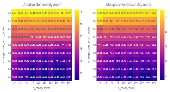
Figure 14.
Grid search using Prophet.
The Prophet approach, which uses a regression model, was applied to analyze the residual signal, which is a time series. The model was trained using data from the first substation, and was then used to study the trend of the residual signal, which mostly consisted of normal points. The approach was evaluated using data from the second substation, where the threshold had to be adjusted due to the presence of more abnormal data. The dynamic threshold, represented by the red line in Figure 15, was found to be better than a static threshold for distinguishing between abnormal and normal states, as it adapts to daily changes in the time series. This technique achieved an MCC score of 0.647 and an ACC score of 0.847.
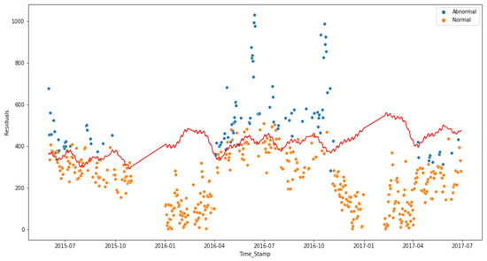
Figure 15.
Time series threshold using Prophet.
The second idea is similar to the first in that it utilizes the residual signal’s seasonality properties. In this approach, the month is used as an independent variable, and the residuals as the output before being fed into an Artificial Neural Network (ANN) model. The monthly forecast value is used as a threshold, as shown in Figure 5. This approach provided a less sensitive threshold than the Prophet threshold and focused only on residual differences over the month, which relies on the nature of the photovoltaic system. Figure 16 shows the dynamic threshold that depends on the month. The result shows that this threshold is entirely reasonable to separate the normal and abnormal states but still has some normal states that the threshold labeled as abnormal. This technique provides an MCC score of 0.671 and an ACC score of 0.849.
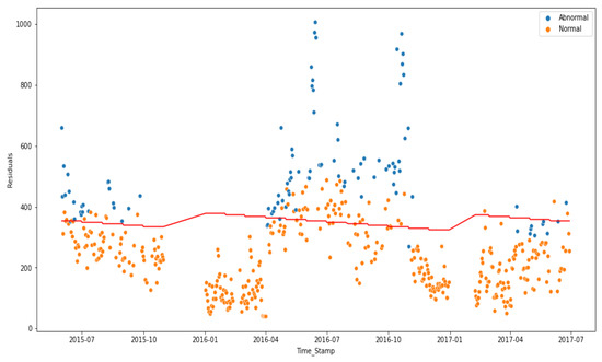
Figure 16.
Monthly threshold using CNN.
After studying the nature of photovoltaic systems, we discovered that they have different levels of energy productivity during different hours of the day. Based on this, we developed a final approach that uses dynamic thresholds based on each hour. For each day, we computed a threshold for each hour based on the 95th percentile of residuals in the same hour over the first substation dataset. It is worth noting that most of the data in the first substation are normal, so the 95th percentile of residuals should represent the maximum criteria of Mean Squared Error (MSE) in normal production. We then labeled each hour as 0 if the residuals were less than the threshold and 1 if the residuals were higher than the threshold. Finally, if the average of the hourly labels was more than 0.5, the day was labeled as abnormal. We tested this approach, and the results are shown in Figure 17. This approach proved to be an interesting and effective way of separating normal and abnormal states, as it obtained the best score, with an MCC score of 0.736 and an ACC score of 0.863. The success of this approach is likely due to its ability to reduce complexity and focus on analyzing each day independently to identify abnormal behaviors.
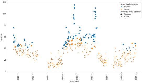
Figure 17.
Hourly vote threshold.
This final experimentation presents a comparison of the average detection scores for each threshold approach. In the report, we evaluated the results using metrics such as MCC, ACC, Precision, Recall, and F1-score. Table 7 shows the comparison of an average detection score between each thresholds. The results of the fault detection approach based on the static threshold developed by Ref. [10] yielded the lowest scores, with an MCC of 0.637 and an ACC of 0.875. However, dynamic thresholds yielded better detection scores than static thresholds. The hourly threshold using the 95th residual’s percentile approach obtained the highest scores, with an MCC score of 0.736 and an ACC score of 0.863. These results may vary depending on the optimization method used; then, we proposed the detection score of five experiments, as shown in Figure 18. However, overall, the hourly threshold using the 95th residual’s percentile approach has proven to be an exceptional method for anomaly detection in photovoltaic systems.
Table 7.
Average detection score of our proposed thresholds in comparison with Ref. [10].
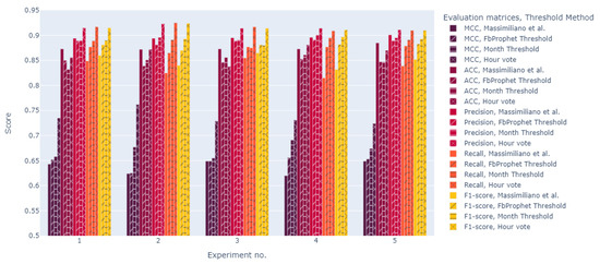
Figure 18.
Various evaluation score comparisons of five experiments [10].
7. Conclusions
Automatic fault detection and diagnosis (FDD) methods are essential for modern PV health monitoring systems. In this study, we proposed a framework for developing fault detection in photovoltaic systems using an indirect method. The pre-researched methodology and the study of the nature of the data have contributed to the experiment. From this step, we obtained a suitable data frequency for the daily data, which show the intrinsic slow dynamic of the solar signals. A suitable residual type is MSE, which is more sensitive to an outlier. Consequently, we confirm the suitable prediction model by experimenting again with various machine learning models. The results of the experiment are reliable with the assumption from previous research that the MLP regressor produced the best classification score, which is higher than the other 10 machine learning models. Nonetheless, static and dynamic thresholds have been investigated for increased performance of automatic fault detection. According to this, the static threshold is imperfect in distinguishing the abnormal scenario from the normal condition. It is better to use a dynamic threshold than a static threshold because a static threshold is not able to capture the relation inside the residual even if it uses energy production prediction. Nonetheless, these dynamic thresholds provide better detection scores because they study the relation between residual and time, which is not only the time between the date as seasonality or time window but also the time in case of each hour in a day.
The results show that all of the proposed dynamic thresholds provide a better score; the hourly threshold using the 95th residual’s percentile gives an outstanding performance at 0.736 MCC and 0.863 balanced ACC. The success of this approach is likely due to its ability to reduce the complexity and focus on analyzing each day independently to identify abnormal behaviors. Furthermore, from this conclusion, we are able to create automatic fault detection, which has hourly and daily notification systems. The key drawback of the created approach is that it only uses one model for all the data. The location, the installation of the sensors, and the size of the solar plant contribute to various irradiance, seasonality, and resolutions. As a result, our goal is to assess and evaluate the accuracy of the current model achieved by dividing it into distinct sub-stations that address the various types of data. The creation of fault classification for significant issues such as dust, hot spots, sensor, or inverter difficulties may also be part of future studies.
Author Contributions
Conceptualization, T.K., W.R. and R.W. (Rabian Wangkeeree); methodology, T.K. and R.W. (Rabian Wangkeeree); software, T.K. and W.R.; validation, T.K.; writing—original draft, T.K.; writing—review and editing, T.K., R.W. (Rabian Wangkeeree), R.W. (Rattanaporn Wangkeeree) and C.S.; supervision, R.W. (Rabian Wangkeeree). All authors have read and agreed to the published version of the manuscript.
Funding
This research has received funding support from the National Science, Research and Innovation Fund (NSRF) and Naresuan University, Thailand, with Grant Number R2565B079.
Acknowledgments
The authors are thankful the referees for their attentive reading and valuable suggestions.
Conflicts of Interest
The authors declare no conflict of interest.
References
- Panwar, N.; Kaushik, S.; Kothari, S. Role of renewable energy sources in environmental protection: A review. Renew. Sustain. Rev. 2011, 15, 1513–1524. [Google Scholar] [CrossRef]
- IEA. Renewables 2020. Available online: https://www.iea.org/reports/renewables-2020 (accessed on 1 May 2022).
- Mellit, A.; Tina, G.; Kalogirou, S. Fault detection and diagnosis methods for photovoltaic systems: A review. Renew. Sustain. Rev. 2018, 91, 1–17. [Google Scholar] [CrossRef]
- Santhakumari, M.; Sagar, N. A review of the environmental factors degrading the performance of silicon wafer-based photovoltaic modules: Failure detection methods and essential mitigation techniques. Renew. Sustain. Rev. 2019, 11, 83–100. [Google Scholar] [CrossRef]
- Peinado Gonzalo, A.; Pliego Marugán, A.; García Márquez, F.P. Survey of maintenance management for photovoltaic power systems. Renew. Sustain. Energy Rev. 2020, 134, 110347. [Google Scholar] [CrossRef]
- Tina, G.M.; Cosentino, F.; Ventura, C. Monitoring and Diagnostics of Photovoltaic Power Plants; Springer International Publishing: Cham, Switzerland, 2016; pp. 505–516. [Google Scholar]
- Burger, B.; Goeldi, B.; Rogalla, S.; Schmidt, H. Module integrated electronics—An overview. In Proceedings of the 25th European Photovoltaic Solar Energy Conference and Exhibition, EU PVSEC 2010, Valencia, Spain, 6–10 September 2010. [Google Scholar]
- Jiang, L.; Maskell, D. Automatic fault detection and diagnosis for photovoltaic systems using combined artificial neural network and analytical based methods. In Proceedings of the 2015 International Joint Conference on Neural Networks (IJCNN), Killarney, Ireland, 12–17 July 2015; pp. 1–8. [Google Scholar]
- Mekki, H.; Mellit, A.; Salhi, H. Artificial neural network-based modelling and fault detection of partial shaded photovoltaic modules. Simul. Model. Pract. Theory 2016, 67, 1–13. [Google Scholar] [CrossRef]
- De Benedetti, M.; Leonardi, F.; Messina, F.; Santoro, C.; Vasilakos, A. Anomaly detection and predictive maintenance for photovoltaic systems. Neurocomputing 2018, 310, 59–68. [Google Scholar] [CrossRef]
- Li, B.; Delpha, C.; Diallo, D.; Migan-Dubois, A. Application of artificial neural networks to photovoltaic fault detection and diagnosis: A review. Renew. Sustain. Energy Rev. 2021, 138, 110512. [Google Scholar] [CrossRef]
- Ibrahim, M.; Alsheikh, A.; Awaysheh, F.M.; Alshehri, M.D. Solar Power Plants Anomaly Detection Using Machine Learning. Energies 2022, 15, 1082. [Google Scholar] [CrossRef]
- Pedregosa, F.; Varoquaux, G.; Gramfort, A.; Michel, V.; Thirion, B.; Grisel, O.; Blondel, M.; Prettenhofer, P.; Weiss, R.; Dubourg, V.; et al. Scikit-learn: Machine learning in python. J. Mach. Learn. Res. 2011, 12, 2825–2830. [Google Scholar]
- Abadi, M.; Agarwal, A.; Barham, P.; Brevdo, E.; Chen, Z.; Citro, C.; Corrado, G.S.; Davis, A.; Dean, J.; Devin, M.; et al. TensorFlow: Large-Scale Machine Learning on Heterogeneous Systems. 2015. Available online: https://www.usenix.org/system/files/conference/osdi16/osdi16-abadi.pdf (accessed on 27 June 2022).
- Gulli, A.; Pal, S. Deep Learning with Keras; Packt Publishing Ltd.: Birmingham, UK, 2017. [Google Scholar]
- Hilt, D.E.; Seegrist, D.W. Ridge: A Computer Program for Calculating Ridge Regression Estimates. Research Note NE-236; U.S. Department of Agriculture, Forest Service, Northeastern Forest Experiment Station: Upper Darby, PA, USA, 1977. [Google Scholar]
- Tibshirani, R. Regression shrinkage and selection via the lasso. J. R. Stat. Soc. 1996, 58, 267–288. [Google Scholar] [CrossRef]
- Zou, H.; Hastie, T. Regularization and variable selection via the elastic net. J. R. Stat. Soc. 2005, 67, 301–320. [Google Scholar] [CrossRef]
- Robbins, H.; Monro, S. A Stochastic Approximation Method. Ann. Math. Stat. 1951, 22, 400–407. [Google Scholar] [CrossRef]
- Kiwiel, K. Convergence and efficiency of subgradient methods for quasiconvex minimization. Math. Program. 2001, 90, 1–25. [Google Scholar] [CrossRef]
- Cortes, C.; Vapnik, V. Support vector networks. Mach. Learn. 1995, 20, 273–297. [Google Scholar] [CrossRef]
- Drucker, H.; Burges, C.J.C.; Kaufman, L.; Smola, A.J.; Vapnik, V. Support vector regression machines. In NIPS; MIT Press: Cambridge, MA, USA, 1996; pp. 155–161. [Google Scholar]
- Vapnik, V.N. The Nature of Statistical Learning Theory; Springer: New York, NY, USA, 1995. [Google Scholar]
- Opitz, D.; Maclin, R. Popular ensemble methods: An empirical study. J. Artif. Intell. Res. 1999, 11, 169–198. [Google Scholar] [CrossRef]
- Polikar, R. Ensemble based systems in decision making. IEEE Circuits Syst. Mag. 2006, 6, 21–45. [Google Scholar] [CrossRef]
- Rokach, L. Ensemble-based classifiers. Artif. Intell. Rev. 2010, 33, 21–45. [Google Scholar] [CrossRef]
- Breiman, L. Bagging predictors. Mach. Learn. 1996, 24, 123–140. [Google Scholar] [CrossRef]
- Breiman, L. Random forests. Mach. Learn. 2001, 45, 5–32. [Google Scholar] [CrossRef]
- Freund, Y.; Schapire, R.E. A decision-theoretic generalization of on-line learning and an application to boosting. J. Comput. Syst. Sci. 1997, 55, 119–139. [Google Scholar] [CrossRef]
- Friedman, J.H. Stochastic gradient boosting. Comput. Stat. Data Anal. 2002, 38, 367–378. [Google Scholar] [CrossRef]
- Hopfield, J.J. Neural networks and physical systems with emergent collective computational abilities. Proc. Natl. Acad. Sci. USA 1982, 79, 2554–2558. [Google Scholar] [CrossRef] [PubMed]
- Kingma, D.P.; Ba, J. Adam. A Method for Stochastic Optimization. Available online: https://arxiv.org/abs/1412.6980 (accessed on 1 April 2022).
- Taylor, S.J.; Letham, B. Forecasting at scale. Am. Stat. 2018, 72, 37–45. [Google Scholar] [CrossRef]
Disclaimer/Publisher’s Note: The statements, opinions and data contained in all publications are solely those of the individual author(s) and contributor(s) and not of MDPI and/or the editor(s). MDPI and/or the editor(s) disclaim responsibility for any injury to people or property resulting from any ideas, methods, instructions or products referred to in the content. |
© 2023 by the authors. Licensee MDPI, Basel, Switzerland. This article is an open access article distributed under the terms and conditions of the Creative Commons Attribution (CC BY) license (https://creativecommons.org/licenses/by/4.0/).