Abstract
Recently, renewable energy resources (RESs) and electric vehicles (EVs), in addition to other distributed energy resources (DERs), have gained high popularity in power systems applications. These resources bring quite a few advantages for power systems—reducing carbon emission, increasing efficiency, and reducing power loss. However, they also bring some disadvantages for the network because of their intermittent behavior and their high number in the grid which makes the optimal management of the system a tough task. Virtual power plants (VPPs) are introduced as a promising solution to make the most out of these resources by aggregating them as a single entity. On the other hand, VPP’s optimal management depends on its accuracy in modeling stochastic parameters in the VPP body. In this regard, an efficient approach for a VPP is a method that can overcome these intermittent resources. In this paper, a comprehensive study has been investigated for the optimal management of a VPP by modeling different resources—RESs, energy storages, EVs, and distributed generations. In addition, a method based on bi-directional long short-term memory networks is investigated for forecasting various stochastic parameters, wind speed, electricity price, load demand, and EVs’ behavior. The results of this study show the superiority of BLSTM methods for modeling these parameters with an error of 1.47% in comparison with real data. Furthermore, to show the performance of BLSTMs, its results are compared with other benchmark methods such as shallow neural networks, support vector machines, and long short-term memory networks.
1. Introduction
1.1. Background and Motivation
Global warming and the energy crisis are the most important problems all around the world; in this regard, the penetration of distributed energy resources (DERs), especially renewable energy sources (RESs) has increased dramatically in the power systems. These resources, on the one hand, bring quite a few advantages such as decreasing pollution and reducing dependency on fossil fuels, but on the other hand, create some challenges for system operators such as increasing uncertainty due to their intermittent behavior [1]. In addition, some methods and technologies are introduced to increase the efficiency of power systems, for instance, using electric vehicles (EVs) and deploying demand response (DR). The most important sources of DR are heating, ventilation, and air conditioning (HVAC) systems, washing machines, and personal computers (PCs), which are expected to have a high portion of usage in the near future (more than 160 TWh of the world’s electricity consumption [2]).
Combining all these aforementioned methods and technologies in the power systems leads to a problem for centralized management in smart grids. Virtual power plants (VPPs), by providing the possibility of decentralized management, are proposed to surmount these challenges [3]. In fact, VPPs aggregate all these small technologies as a single entity to get the most out of DERs. Furthermore, VPPs enable small-scale resources to participate in the wholesale electricity markets [4]. Nowadays, VPPs are faced with a big challenge in participating in the electricity market—forecasting different uncertainties in the VPP’s body with good accuracy. Therefore, it is vital to use reliable methods for modeling these uncertainties.
1.2. Literature Survey
Conquering the above-mentioned challenges with papers in the literature can be divided into two groups. The first group of papers has addressed how to solve the VPP energy management problem which benefits from different resources. Study [5] uses an imperialist competitive algorithm for the energy management of a VPP; however, load flow constraints and emission costs are not taken into account without modeling load flow and the constraints of the network. Moreover, the results of the study are not realistic and the advantages of RESs are not visible properly because the emission cost is not modeled in this work. A solution for the management of a VPP by involving risk is implemented in [2] to minimize costs by considering correlated DR; EVs are not modeled in this study. By considering the current trend of power systems, EVs are the inseparable part of the future networks. In study [6], the optimal scheduling of a VPP includes DERs and DR without modeling energy storages (ESs) using meta-heuristic algorithms. Meta-heuristic algorithms have a high computational cost in addition to the possibility of stocking in local optimal points. Sadeghi et al. [3] have presented an optimal bidding strategy for VPPs in the day-ahead energy and frequency regulation markets. In study [7], the problem is solved to reduce the carbon emission to maximize profit, but EVs are not investigated and load flow constraints are not taken into account. Study [8] conducted the planning of a technical VPP for contingency conditions such as single-line outages and seasonal load change but ESs, EVs, and emission costs are not studied. The alternating direction method of multipliers is developed in [9] for optimal dispatch of a VPP consisting of conventional distributed generations (DGs), i.e., fossil fuel-based units, RESs, ESs, and interruptible load. Optimal participation of a VPP in energy and spinning reserve markets has been conducted in [10] without modeling the impact of uncertainty modeling on the VPP’s optimal bidding in the day-ahead (DA) market. In addition, this work is not utilized in the DR program. DR can effectively reduce the total cost and peak demand in the VPP. In study [11] the conditional value at risk (CVaR) is utilized for modeling the risk of a VPP but the impact of EVs is not investigated. Daily and weekly scheduling of a VPP is conducted in [12] by the robust optimization method; however, this work has not investigated most of the main resources in VPPs such as ESs and EVs. A game theory-based approach based on the supply function Nash equilibrium and shapely value is conducted in [13] for optimal participation of a VPP as a price maker unit in the market. Optimal bidding of a VPP including EVs, RESs, TSs, and ESs in the day-ahead and the balancing market has been conducted in [14]; however, the DR program is not utilized. In study [4], the impact of a DR program for participating a VPP in the electricity market is studied but this method is based on a MINLP formulation and does not consider EVs. In study [15], the planning and operation of VPPs in the market are modeled by considering uncertainties but the proposed method is not investigated regarding EVs, load flow, emission cost, and DG constraints. A VPP, as a case study in India for the integration of RESs, is presented in [16]; however, this paper, as shown in Table 1, does not model some important sources and constraints. Further resources are explained in Table 1. A comparison among existing papers from an optimal management strategy’s point of view is presented in Table 1.

Table 1.
A survey for VPPs’ energy management in the existing literature.
In the second group of papers, various models are utilized for modeling different stochastic parameters. In study [18], a solution for the management of a VPP by considering EVs is proposed. This work has not modeled both the EVs’ stochastic behavior and RES uncertainty. The EVs’ behavior and electricity price uncertainties have not been taken into account in [19] although a Markov model is used for RES uncertainty. A scenario-based method is investigated in [8]; these scenarios were created by using Normal and Weibull distribution functions. In scenario-based methods to reach a high accuracy, a multitude of scenarios is required which increases the computational cost of the problem. In studies [5,15,20], the 2-point estimate method (PEM) has been used to model uncertainties. PEM cannot bring a high accuracy in datasets with large fluctuations in wind speed and electricity price [22]. In study [20], autoregressive moving average series (ARMA) is utilized in addition to the adaptive neuro-fuzzy inference system for modeling price and wind uncertainties, respectively. Study [6] has used Weibull, Beta, and Normal distribution functions for modeling uncertainty in WT, photovoltaics, and EVs, respectively. The same method is employed in [7] and [11]. In study [10], long short-term memory (LSTM) networks are applied for modeling different stochastic parameters; however, a rough artificial neural network (RANN) is considered for modeling EVs’ behaviors without considering the relationship among different features such as arrival time, departure time, and travel distance which increases the number of infeasible samples. In study [23], the authors the authors proposed optimal bidding for EVs and ES aggregators in the day-ahead market (DAM) for the frequency regulation market where the uncertainty in price is modeled by the seasonal autoregressive moving average (SARIMA) model, and load uncertainty is not considered. Study [24] does not model the uncertainty in the electricity price. Based on the information which is presented in Section 1.2 and Table 1 and Table 2, the knowledge gap for this subject can be summarized as follows:
Table 2.
A survey of methods for modeling stochastic parameters in VPPs.
- Based on the current trends in the power systems and disadvantages of fossil fuel-based units, considering DR programs and EVs are necessary. In addition, the emission cost is a vital factor for increasing the penetration of RESs that should be investigated in the studies for optimal management of VPPs. Therefore, modeling a comprehensive study by considering all the components indicated in Table 1 is essential and has not been completely considered by any of the reviewed papers.
- Modeling uncertainties, especially EVs’ behavior owing to the fact that VPPs have a high percentage of stochastic resources can completely change the bids of VPPs in the market. In this regard, using methods with high accuracy based on data-driven approaches plays a decisive role to decrease the penalty cost of VPPs in the electricity market.
1.3. Paper Contribution
Based on the comparison in Table 1 and Table 2, the main goal of this paper is to provide a comprehensive study for a technical VPP—containing different resources including DG, WT, ES, EVs, and DR—with the aim of minimizing total cost by taking into account the network and unit constraints. The overall structure of the proposed method is depicted in Figure 1, considering different resources in the VPP body can increase the efficiency of VPPs and strengthen their coalition. In addition, WTs can reduce carbon emissions, and ESs are used to cover uncertainty in RESs and peak shaving. Furthermore, ES’s degradation cost is modeled in this paper to increase the practicality of the proposed method. The emission cost of fossil fuel-based units is investigated to reduce the global warming effects and pave the way to increase the penetration of RESs. In addition, a method based on BLSTM networks is applied to model all the uncertainties associated with the optimal management of a VPP. For implementing the effect of this method for modeling stochastic parameters, the participation of a VPP in DAM is investigated. In summary, the main contributions of this paper are as follows:
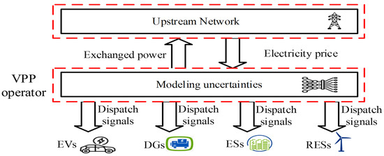
Figure 1.
Structure of the proposed method.
- Forecasting all uncertainties involved in the planning of a VPP by bi-directional long short-term memory (BLSTM) networks—load, price, RES, and EV uncertainties. Furthermore, in this paper, EV samples are generated based on three features (arrival time, departure time, and travel distance) by considering dependency among these features. However, other works considered them separately or used the Monte Carlo method which cannot effectively model EVs’ behavior and increased the number of infeasible samples.
- Proposing a comprehensive mixed-integer linear programming (MILP) model for technical VPPs’ energy management, by emission cost, network and unit constraints, DR, and degradation cost of ES.
- Considering the VPP participation in DAM.
1.4. Paper Organization
2. Problem Formulation
The objective function of the VPP in this paper is to minimize the total cost as presented in Equation (1). In this paper, it is supposed that VPP is a price-taking unit in the market.
The VPP cost function includes the cost of active exchanged power with the upstream distribution network, DG, ES, and WT costs, respectively. indicates the amount of active power exchange with the upstream network at hour t—positive values indicate the active power is purchased from the network and the negative values indicate the active power is sold to the network. Equation (2) shows the maximum allowable active power which can be exchanged with the upstream network.
DG constraints are presented in Equations (3)–(18) [10,30]. Equation (3) shows the DG cost function which includes the fuel, emission, startup, and shutdown costs. The fuel cost function is a quadratic function in the general formula which, in this paper, is linearized based on a piecewise linear method [30]. Equation (4) indicates the amount of generated power by each DG. Equation (5) shows the emission cost [10]. Equations (6) and (7) relate to the minimum and maximum limit of active and reactive generated power by DGs; Equations (8) and (9) demonstrate ramping up and down limits. Equations (10)–(15) indicate the minimum up and minimum downtime limits; these equations indicate how much time a DG should remain off or on when it turns off or turns on. In addition, Equations (16)–(18) are used for linearization.
The following equations describe ES’s operation [31]:
Equation (19) indicates ES cost at time t which is calculated based on the amount of ES charging and discharging. In Equation (20), the amount of injected or received power by ES is indicated; Equations (21) and (22) show upper and lower limits of charging and discharging per hour. Equation (23) indicates the state of charging or discharging in each hour because the ES can only have one charging or discharging state. Equations (24) and (25) represent the level of SOC per hour, and Equation (26) refers to the maximum and minimum SOC per hour.
Equations (27)–(31) are used to model EVs [23]. EVs are divided into unidirectional and bi-directional vehicles. Since bi-directional V2G requires complex protection and power electronic hardware, and is not economically feasible for implementation in the residential grids with the current technology [23], in this paper, we consider unidirectional EVs.
where, Equation (27) shows the amount of power consumed for charging EV batteries, which depends on the rated charger capacity; Equations (28) and (29) are used to calculate the SOC of EVs, and Equation (30) shows the maximum SOC of EVs. Finally, Equation (31) is applied to ensure EVs’ SOC is more than 90% in the departure time.
WT cost is indicated in Equation (32); the power output of WTs depends on the wind speed as explained in [32].
For modeling load flow, we used linear load flow formulation as in study [33]:
Equations (34) and (35) apply active and reactive power balance in each bus; Equations (36) and (37) express the amount of active and reactive power generation at each bus. Equations (38)–(40) demonstrate active, reactive, and apparent power flow of lines, correspondingly. Equations (41) and (42) enforce bus voltages and apparent power of line in the desired range. Equations (43)–(46) are investigated for modeling the DR program. Equations (43) and (44) show the amount of increase or decrease in the load demand in bus b and time t. The sum of the total increase in load in each bus in 24 h should be equal to some of the decrease which is controlled by Equation (45). Finally, Equation (46) shows the load after implementing the DR program.
3. Numerical Results
3.1. Input Data
To investigate the efficiency of the proposed method, a VPP as shown in Figure 2 is considered as the case study. Network information is presented in study [34]. The VPP consists of four DGs, two ESs, and two WTs which are located at various buses in accordance with Figure 2. The VPP is connected to the upstream distribution network at bus 1. In this study, 200 EVs are connected to different load buses. The data from ESs, DGs, emission, and WTs are presented in Table 3, Table 4, Table 5 and Table 6. Emission data were selected based on [35].
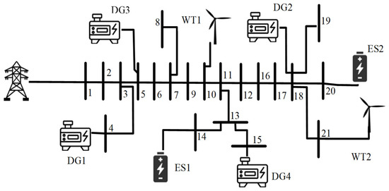
Figure 2.
Overall structure of the case study.
Table 3.
ESs’ data.
Table 4.
DGs’ data.
Table 5.
Emission data.
Table 6.
WTs’ data.
3.2. Uncertainty Modeling
For modeling the different stochastic data, the BLSTM method is utilized. BLSTMs have been known as a promising tool for time series forecasting. The formulation of BLSTMs is explained in [22]. The overall structure of the BLSTM method for forecasting these uncertainties is shown in Figure 3. For the dataset, we used data from Ontario, a province in Canada [36]. The data for three years (2019–2021) were selected as the database. The dataset was divided by 80%, 10%, and 10% as the training, validation, and test sets. In addition, for EVs’ data, the data from the National Household Travel Survey (NHTS) were used and for forecasting each sample, three features: arrival, departure, and travel distance were taken into account. In this way, the connection among features is considered which decreases the number of infeasible samples.

Figure 3.
Overall structure of the BLSTM method.
As it is depicted in Figure 4, the BLSTM method is close to the real data in comparison with other methods for forecasting different parameters. To better clarify this in the next section, the numerical results and costs are presented for various methods. To provide a quantitative comparison and more perceptible results, the accuracy of the BLSTM network is compared with other methods by calculating two well-known error criteria, including the mean absolute error (MAE), and the root mean square error (RMSE) [36] which is presented in Table 7. The results of this table beside the graphs in Figure 4 clearly show the superiority of the BLSTM method in comparison to other benchmark methods. In the time series forecasting task, the deviations between real data and forecasted values depend on the accuracy of the forecasting method. For example, for load demand, which has a smoother trend, the deviations are low among real data and all forecasting methods. However, for data with high fluctuations, such as wind speed deviations, are high compared to real data for different methods. For instance, BLSTM has the lowest deviations with real data and LSVM has the highest. To better clarify this issue, all this information is added to the paper.
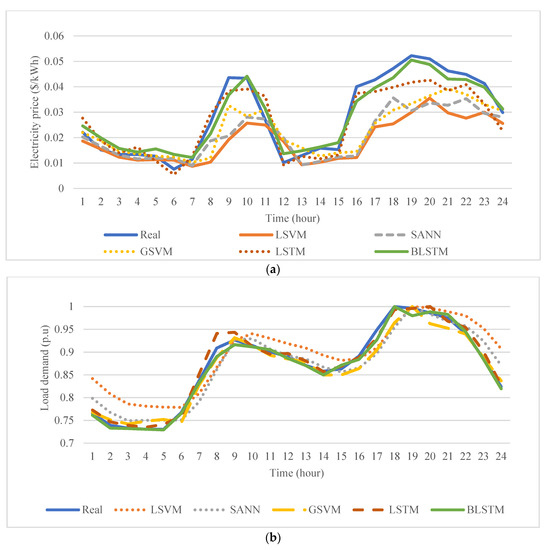
Figure 4.
Forecasted values and their comparison with the real data: (a) electricity price; (b) load demand; (c) wind speed.
Table 7.
Forecasting error criteria for different methods.
3.3. Case Study Results
The optimization problem is implemented for the case study. In order to show the advantage of BLSTMs for modeling different stochastic parameters and their effect on the total cost of the VPP, the results of BLSTM are compared with real data, and several benchmark methods such as LSTM, shallow artificial neural networks (SANN), linear support vector machine (LSVM), and Gaussian support vector machine (GSVM).
Figure 5 shows the exchange power between the VPP and the upstream network. As can be seen, the most similarity exists between the real data and the BLSTM method, which makes the cost of the VPP more closely related to the actual cost and optimal utilization of resources, while other methods, due to their lesser ability in modeling uncertainties, cause a large difference in actual and scheduled amounts. The reason why the VPP buys electricity from the upstream network all over the hours is that the capacity of the resources in the VPP is less than its load. Additionally, as shown in Figure 5, the VPP in the early hours of the day when the electricity price is low received more power from the network and, with increasing electricity prices, the amount of power received from the upstream network decreased; especially, at hours 9–10 and 18–23 where the electricity price is too high, the VPP has received the lowest power from the network.
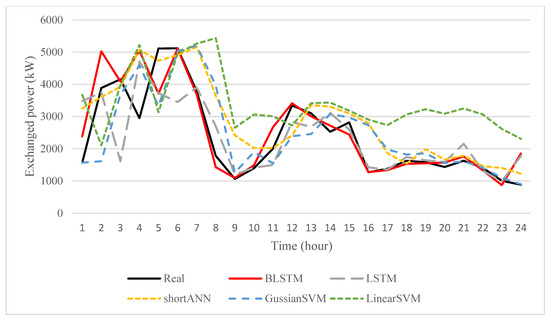
Figure 5.
Amount of exchanged power between VPP and upstream network.
ESs’ SOC is shown in Figure 6. As it is evident from this figure, ESs start to discharge in the early hours of the day when the load is low to charge EVs, and continues to charge in the next hours, so that it can reduce the peak load in hours 9–11 and 19–22 by discharging.
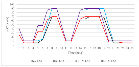
Figure 6.
SOC of ESs with real data and BLSTM method.
The amount of generated power by each DG in 24 h for real data are compared with those of the BLSTM method given in Figure 7. As illustrated in this figure, in hours 1–7, the amount of load and also the electricity prices are low, therefore, the VPP will keep the DGs in their minimum capacity due to the high cost of DGs (because the emission cost is taken into the problem) and buy more power from the network. With rising prices as well as rising loads at hours 9–10 and 16–23, DGs work at their maximum production capacity to reduce the purchasing power from the network due to high electricity prices.
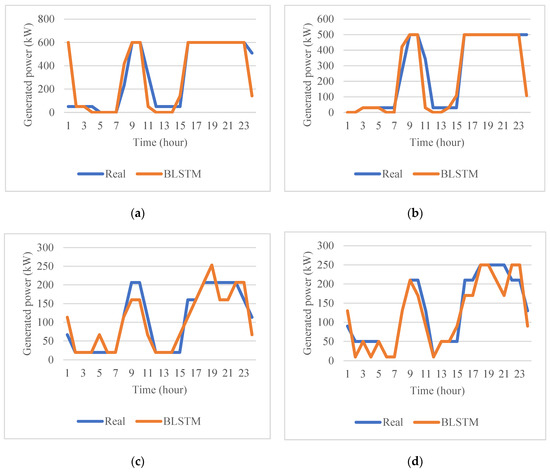
Figure 7.
Generated power (kW) by DGs in 24 h for real data and BLSTM methods: (a) DG1; (b) DG2; (c) DG3; (d) DG4.
Figure 8 shows the amount of EVs which are charging for real data and the BLSTM method, which are very close together. Additionally, to investigate the effect of coordinated and uncoordinated EV charging—EVs start charging after entering the parking lot—on the network, the proposed algorithm was implemented once for coordinated charging (Figure 9) and again for uncoordinated charging (Figure 10) on real data.

Figure 8.
EVs charging in the coordinate charging procedure for real data and BLSTM method.
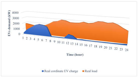
Figure 9.
Impact of coordinated charging on the network load.
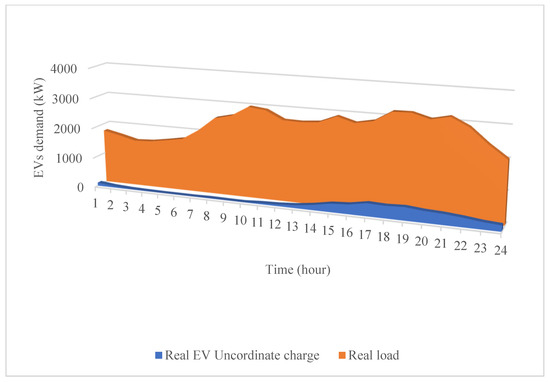
Figure 10.
Impact of uncoordinated charging on the network load.
As illustrated in Figure 9 and Figure 10, in the case of coordinate charging, the VPP adjusts the EV charging to the early hours of the day when the load is low, thereby it prevents the synchronization of the residential pick load and charging of EVs, which reduces the tensions on the network. It is also economical for the owners of the EVs because EV charging is conducted at low electricity prices which reduces the charging cost for EVs’ owners. However, in uncoordinated charging mode due to the synchronization of EVs’ charging and the residential peak load, the tension entered into the network increases and may even cause network instability.
In Table 8, details of the cost of the VPP for real data as well as the forecasted data by five other methods are presented. As stated in this table, the BLSTM method has the lowest error in comparison with other methods (1/47% error), which demonstrates the effectiveness of this method to forecast various uncertainties. In other methods, the cost is different from the actual cost and is much lower than the actual cost, which makes the VPP unable to properly estimate its costs. Therefore, it must pay a heavier penalty, and cannot bid optimally on the DAM.
Table 8.
VPP costs in different methods.
4. Conclusions
In this paper, a complete model is presented for the optimal management of a VPP in day-ahead markets with modeling uncertainties. This method is based on a mixed-integer linear programming which is suitable for large-scale problems. The characteristics of the proposed method are considering renewable energy resources, electric vehicles, distributed generations, and energy storages in the VPP body. Considering these components plays a decisive role for VPPs because the concept of a VPP is proposed to aggregate these small energy resources to overcome the challenges of future power systems. In addition, owing to the fact that modeling stochastic parameters play a crucial role in the optimal management of VPPs, a method based on deep bi-directional long short-term memory networks is investigated for forecasting these parameters. The results of this study are compared to other benchmark methods—shallow neural networks, support vector machines, and long short-term memory networks—to show the dominance of the proposed method against other methods. The results of the study show BLSTMs can closely forecast the parameters by causing only a 1.47% error compared to real data whereas other methods have an error of more than 10%.
Author Contributions
Conceptualization, A.A. (Ali Ahmadian), K.P. and A.E.; methodology, A.A. (Ali Ahmadian) and K.P.; software, A.A. (Ali Ahmadian); validation, A.A. (Ali Ahmadian), K.P., A.A. (Ali Almansoori), and A.E.; formal analysis, A.A. (Ali Ahmadian), K.P. and A.E.; investigation, A.A. (Ali Ahmadian); validation, A.A. (Ali Ahmadian), K.P., A.A. (Ali Almansoori), and A.E.; resources, A.A. (Ali Ahmadian); data curation, A.A. (Ali Ahmadian); validation, A.A. (Ali Ahmadian), K.P., A.A. (Ali Almansoori), and A.E.; writing—original draft preparation, A.A. (Ali Ahmadian); writing—review and editing, A.A. (Ali Ahmadian); validation, A.A. (Ali Ahmadian), K.P., A.A. (Ali Almansoori), and A.E.; visualization, A.A.(Ali Ahmadian); supervision, K.P. and A.E.; project administration, A.E.; funding acquisition, A.E. All authors have read and agreed to the published version of the manuscript.
Funding
This research received no external funding.
Data Availability Statement
There is no new data.
Conflicts of Interest
The authors declare no conflict of interest.
Nomenclature
| Indices | |
| Time index | |
| Conventional distributed generation (DG) index | |
| Wind turbine (WT) index | |
| Emission type index | |
| Index for linear pieces | |
| Energy storages (ESs) index | |
| Nodes indices | |
| Electric vehicles (EVs) index | |
| Parameters | |
| Start-up cost ($) | |
| Externality costs | |
| Emission factor | |
| , | ESs’ charging and discharging efficiency |
| Rated charger capacity (kW) | |
| EVs’ charging efficiency | |
| Initial state of charge (SOC) of EVs (kWh) | |
| EVs’ battery capacity (kWh) | |
| Active power demand (kW) | |
| Conductance value of line bl (p.u) | |
| Reactive power demand (kVar) | |
| Linear load flow constant | |
| Coefficient for WT cost ($/kW) | |
| Maximum output power of WTs (kW) | |
| , | Minimum up and down times (h) |
| , | Minimum and maximum output power of DGs (kW) |
| ,, | DG cost coefficients |
| , | ES cost coefficients |
| , | Minimum and maximum SOC of ESs (kWh) |
| , | Maximum and minimum charge rate of ESs (kW) |
| Susceptance value of line bl (p.u) | |
| Maximum magnitude of apparent power flow (kVA) | |
| , | Minimum and maximum voltage limit (p.u) |
| , , | Cut-in, cut-out, and rated speed of WTs |
| Base apparent power (kVA) | |
| Active power price in day-ahead market (DAM) at hour t ($/kw) | |
| Maximum allowable exchanged power with upstream network | |
| Shut down cost ($) | |
| , | Ramp-up and ramp-down rate limits (kW) |
| Wind speed | |
| Slope of piece-line k | |
| Big value | |
| Variables | |
| DG cost ($) | |
| Amount of active exchanged power with the upstream network (kW) | |
| Emission cost ($) | |
| , | Binary variable for the commitment of DGs |
| ES cost ($) | |
| WT cost ($) | |
| , | Maximum allowable amount for increasing or decreasing load in each bus (kW) |
| OFF and ON time of DGs (h) | |
| , | Generated active and reactive power by unit m |
| Generated power in segment k (kW) | |
| , | Amount of ESs’ charging and discharging (kW) |
References
- Dehghani, M.; Taghipour, M.; Sadeghi Gougheri, S.; Nikoofard, A.; Gharehpetian, G.B.; Khosravy, M. A Deep Learning-Based Approach for Generation Expansion Planning Considering Power Plants Lifetime. Energies 2021, 14, 8035. [Google Scholar] [CrossRef]
- Liang, Z.; Alsafasfeh, Q.; Jin, T.; Pourbabak, H.; Su, W. Risk-Constrained Optimal Energy Management for Virtual Power Plants Considering Correlated Demand Response. IEEE Trans. Smart Grid 2017, 10, 1577–1587. [Google Scholar] [CrossRef]
- Sadeghi, S.; Jahangir, H.; Vatandoust, B.; Golkar, M.A.; Ahmadian, A.; Elkamel, A. Optimal bidding strategy of a virtual power plant in day-ahead energy and frequency regulation markets: A deep learning-based approach. Int. J. Electr. Power Energy Syst. 2021, 127, 106646. [Google Scholar] [CrossRef]
- Ullah, Z.; Hassanin, H. Modeling, optimization, and analysis of a virtual power plant demand response mechanism for the internal electricity market considering the uncertainty of renewable energy sources. Energies 2022, 15, 5296. [Google Scholar] [CrossRef]
- Kasaei, M.J.; Gandomkar, M.; Nikoukar, J. Optimal management of renewable energy sources by virtual power plant. Renew Energy 2017, 114, 1180–1188. [Google Scholar] [CrossRef]
- Ju, L.; Li, H.; Zhao, J.; Chen, K.; Tan, Q.; Tan, Z. Multi-objective stochastic scheduling optimization model for connecting a virtual power plant to wind-photovoltaic-electric vehicles considering uncertainties and demand response. Energy Convers Manag. 2016, 128, 160–177. [Google Scholar] [CrossRef]
- Ju, L.; Tan, Q.; Lu, Y.; Tan, Z.; Zhang, Y.; Tan, Q. A CVaR-robust-based multi-objective optimization model and three-stage solution algorithm for a virtual power plant considering uncertainties and carbon emission allowances. Int. J. Electr. Power Energy Syst. 2019, 107, 628–643. [Google Scholar] [CrossRef]
- Hooshmand, R.-A.; Nosratabadi, S.M.; Gholipour, E. Event-based scheduling of industrial technical virtual power plant considering wind and market prices stochastic behaviors-A case study in Iran. J. Clean Prod. 2018, 172, 1748–1764. [Google Scholar] [CrossRef]
- Chen, G.; Li, J. A fully distributed ADMM-based dispatch approach for virtual power plant problems. Appl. Math Model. 2018, 58, 300–312. [Google Scholar] [CrossRef]
- Gougheri, S.S.; Jahangir, H.; Golkar, M.A.; Ahmadian, A.; Aliakbar Golkar, M. Optimal participation of a virtual power plant in electricity market considering renewable energy: A deep learning-based approach. Sustain. Energy Grids Netw. 2021, 26, 100448. [Google Scholar] [CrossRef]
- Tan, Z.; Wang, G.; Ju, L.; Tan, Q.; Yang, W. Application of CVaR risk aversion approach in the dynamical scheduling optimization model for virtual power plant connected with wind-photovoltaic-energy storage system with uncertainties and demand response. Energy 2017, 124, 198–213. [Google Scholar] [CrossRef]
- Shabanzadeh, M.; Sheikh-El-Eslami, M.-K.; Haghifam, M.-R. The design of a risk-hedging tool for virtual power plants via robust optimization approach. Appl. Energy 2015, 155, 766–777. [Google Scholar] [CrossRef]
- Gougheri, S.S.; Dehghani, M.; Nikoofard, A.; Jahangir, H.; Golkar, M.A. Economic assessment of multi-operator virtual power plants in electricity market: A game theory-based approach. Sustain. Energy Technol. Assess. 2022, 53, 102733. [Google Scholar] [CrossRef]
- Zhou, B.; Liu, X.; Cao, Y.; Li, C.; Chung, C.Y.; Chan, K.W. Optimal scheduling of virtual power plant with battery degradation cost. IET Gener. Transm. Distrib. 2016, 10, 712–725. [Google Scholar] [CrossRef]
- Ullah, Z.; Hassanin, H.; Cugley, J.; Alawi, M.A. Planning, Operation, and Design of Market-Based Virtual Power Plant Considering Uncertainty. Energies 2022, 15, 7290. [Google Scholar] [CrossRef]
- Sharma, H.; Mishra, S.; Dhillon, J.; Sharma, N.K.; Bajaj, M.; Tariq, R.; Rehman, A.U.; Shafiq, M.; Hamam, H. Feasibility of Solar Grid-Based Industrial Virtual Power Plant for Optimal Energy Scheduling: A Case of Indian Power Sector. Energies 2022, 15, 752. [Google Scholar] [CrossRef]
- Hu, J.; Liu, Y.; Jiang, C. An optimum bidding strategy of CVPP by interval optimization. IEEJ Trans. Electr. Electron Eng. 2018, 13, 1568–1577. [Google Scholar] [CrossRef]
- Barati, H.; Ashir, F. Managing and Minimizing Cost of Energy in Virtual Power Plants in the Presence of Plug-in Hybrid Electric Vehicles Considering Demand Response Program. J. Electr. Eng. Technol. 2018, 13, 568–579. [Google Scholar]
- Iacobucci, R.; McLellan, B.; Tezuka, T. Costs and carbon emissions of shared autonomous electric vehicles in a Virtual Power Plant and Microgrid with renewable energy. Energy Procedia 2019, 156, 401–405. [Google Scholar] [CrossRef]
- Abbasi, M.H.; Taki, M.; Rajabi, A.; Li, L.; Zhang, J. Coordinated operation of electric vehicle charging and wind power generation as a virtual power plant: A multi-stage risk constrained approach. Appl. Energy 2019, 239, 1294–1307. [Google Scholar] [CrossRef]
- Zhang, G.; Jiang, C.; Wang, X.; Li, B.; Zhu, H. Bidding strategy analysis of virtual power plant considering demand response and uncertainty of renewable energy. IET Gener. Transm. Distrib. 2017, 11, 3268–3277. [Google Scholar] [CrossRef]
- Jahangir, H.; Tayarani, H.; Gougheri, S.S.; Golkar, M.A.; Ahmadian, A.; Elkamel, A. Deep Learning-based Forecasting Approach in Smart Grids with Micro-Clustering and Bi-directional LSTM Network. IEEE Trans. Ind. Electron. 2020, 68, 8298–8309. [Google Scholar] [CrossRef]
- Vatandoust, B.; Ahmadian, A.; Golkar, M.A.; Elkamel, A.; Almansoori, A.; Ghaljehei, M. Risk-Averse Optimal Bidding of Electric Vehicles and Energy Storage Aggregator in Day-ahead Frequency Regulation Market. IEEE Trans. Power Syst. 2018, 34, 2036–2047. [Google Scholar] [CrossRef]
- Yao, E.; Wong, V.W.S.; Schober, R. Optimization of aggregate capacity of PEVs for frequency regulation service in day-ahead market. IEEE Trans. Smart Grid 2016, 9, 3519–3529. [Google Scholar] [CrossRef]
- Zamani, A.G.; Zakariazadeh, A.; Jadid, S. Day-ahead resource scheduling of a renewable energy based virtual power plant. Appl. Energy 2016, 169, 324–340. [Google Scholar] [CrossRef]
- Zamani, A.G.; Zakariazadeh, A.; Jadid, S.; Kazemi, A. Stochastic operational scheduling of distributed energy resources in a large scale virtual power plant. Int. J. Electr. Power Energy Syst. 2016, 82, 608–620. [Google Scholar] [CrossRef]
- Hadayeghparast, S.; Farsangi, A.S.; Shayanfar, H. Day-ahead stochastic multi-objective economic/emission operational scheduling of a large scale virtual power plant. Energy 2019, 172, 630–646. [Google Scholar] [CrossRef]
- Lima, R.M.; Conejo, A.J.; Langodan, S.; Hoteit, I.; Knio, O.M. Risk-averse formulations and methods for a virtual power plant. Comput. Oper. Res. 2018, 96, 350–373. [Google Scholar] [CrossRef]
- Yi, Z.; Xu, Y.; Gu, W.; Wu, W. A Multi-time-scale Economic Scheduling Strategy for Virtual Power Plant Based on Deferrable Loads Aggregation and Disaggregation. IEEE Trans. Sustain. Energy 2019, 11, 1332–1346. [Google Scholar] [CrossRef]
- Gougheri, S.S.; Jahangir, H.; Golkar, M.A.; Moshari, A. Unit Commitment with Price Demand Response based on Game Theory Approach. In Proceedings of the 2019 International Power System Conference (PSC), Tehran, Iran, 9–11 December 2019; IEEE: Piscataway, NJ, USA, 2019; pp. 234–240. [Google Scholar]
- Sedghi, M.; Ahmadian, A.; Golkar, M.A. Optimal storage planning in active distribution network considering uncertainty of wind power distributed generation. IEEE Transactions on Power Systems. 2015, 31, 304–316. [Google Scholar] [CrossRef]
- Ghaljehei, M.; Ahmadian, A.; Golkar, M.A.; Amraee, T.; Elkamel, A. Stochastic SCUC considering compressed air energy storage and wind power generation: A techno-economic approach with static voltage stability analysis. Int. J. Electr. Power Energy Syst. 2018, 100, 489–507. [Google Scholar] [CrossRef]
- Manshadi, S.D.; Khodayar, M.E. Resilient operation of multiple energy carrier microgrids. IEEE Trans. Smart Grid 2015, 6, 2283–2292. [Google Scholar] [CrossRef]
- Sedghi, M.; Ahmadian, A.; Pashajavid, E.; Aliakbar-Golkar, M. Storage scheduling for optimal energy management in active distribution network considering load, wind, and plug-in electric vehicles uncertainties. J. Renew Sustain. Energy 2015, 7, 33120. [Google Scholar] [CrossRef]
- Mohamed, F.A.; Koivo, H.N. System modelling and online optimal management of microgrid using mesh adaptive direct search. Int. J. Electr. Power Energy Syst. 2010, 32, 398–407. [Google Scholar] [CrossRef]
- Jahangir, H.; Tayarani, H.; Baghali, S.; Ahmadian, A.; Elkamel, A.; Golkar, M.A.; Castilla, M. A Novel Electricity Price Forecasting Approach Based on Dimension Reduction Strategy and Rough Artificial Neural Networks. IEEE Trans. Ind. Informat. 2019, 16, 2369–2381. [Google Scholar] [CrossRef]
Disclaimer/Publisher’s Note: The statements, opinions and data contained in all publications are solely those of the individual author(s) and contributor(s) and not of MDPI and/or the editor(s). MDPI and/or the editor(s) disclaim responsibility for any injury to people or property resulting from any ideas, methods, instructions or products referred to in the content. |
© 2023 by the authors. Licensee MDPI, Basel, Switzerland. This article is an open access article distributed under the terms and conditions of the Creative Commons Attribution (CC BY) license (https://creativecommons.org/licenses/by/4.0/).