Abstract
A dynamic simulation model of a heliostat field and molten salt receiver system are developed on the STAR-90 simulation platform. In addition, a real-time simulation model coupling the above two models is built to study the photothermal conversion process of Delingha’s 50 MW solar power tower plant. The nonuniform and time-varying characteristics of the energy flux density on the receiver surface and the dynamic characteristics under different operating conditions are studied. The operational process of the receiver of a typical day is simulated. It was found that there was a strong positive correlation between the energy flux and DNI, and the maximum energy flux density on the surface of the heat absorbing tube panel moved from the first tube panel to the fourth in sequence from 12:00 to 18:00. At the same time, the energy flux density of the last four panels decreased gradually along the arrangement order of the panels. DNI, molten salt mass flow rate and inlet temperature step disturbance simulations are carried out, and the response curves of the molten salt outlet temperature and tube wall temperature are obtained. The conclusion of this paper has important guiding significance for the establishment of an operational strategy for photothermal coupling in a molten salt solar power tower plant.
1. Introduction
With the rapid development of the world economy in recent years, the problems of energy consumption and shortage are becoming increasingly serious. According to world energy statistics, China, for 18 consecutive years, ranked first in global energy consumption growth, while industrial consumption accounted for more than 70% [1]. How to reduce the consumption of fossil fuels has once again been put on the agenda, and the power and heat industries have been greatly impacted. Since then, China has focused on making renewable energy the mainstay of its new power system, controlling fossil energy consumption and reducing greenhouse gases.
However, there are many problems in the development of renewable energy power generation. Energy absorption is a key problem to be solved, but the concept of the “integration of wind, solar and thermal storage” may solve the power grid coordination problem [2]. Renewable energy generation is usually characterized by low energy density, intermittency and geographical constraints, which greatly restrict its efficient and large-scale development [3,4]. The development of an energy storage system can mitigate the impact of intermittency and help to realize uninterrupted power generation. The volatility of renewable energy makes it necessary to cooperate with energy storage technology to achieve peak-filling purposes. Energy storage technologies will serve as the cornerstone of renewable energy integration [5].
In the field of energy and electricity, solar energy is favored for its cleanness, long duration and great radiant energy. Molten salt solar power tower (SPT) technology with good dispatchability is equipped with thermal storage systems to help it achieve continuous power generation. This renewable energy generation technology will be widely used in the future in new power systems. At present, there are still many technical problems in the operation of an SPT plant, which need to be constantly explored. The energy flux density on the receiver surface is very uneven, which will seriously affect the safe operation of the receiver to a certain extent [6]. In order to reduce the influence of nonuniform energy fluxes on the operation of the receiver, most researchers focus on simulating the distribution of a solar flux. Qiu [7] developed a model to simulate the operation of the receiver in the Dahan power station and obtained the solar flux distribution on the heat absorbing tube in the receiver. Cruz et al. [8] developed an optimization algorithm to equalize the energy flux density on the endothermic surface of a receiver. Xu et al. [9] established a three-dimensional transient model and calculated the temperature field of the receiver under the time-varying flux to simulate the transient characteristics of the receiver. Sanchez et al. [10] studied the nonuniform energy flux distribution on an external receiver. Ho [11] used the photographic flux (PHLUX) mapping method to determine the distribution of a solar flux from a concentrating system. Besarati et al. [12] proposed a new optimization algorithm and combined it with the HFLCAL model for verification, finding that the new algorithm can effectively reduce the maximum energy flux density. In previous studies, more attention has been paid to the energy flux distribution of the cavity receiver, but the research on the external receiver cannot be neglected. The energy flux on the surface of the receiver is usually measured by infrared thermography, but the direct normal irradiance (DNI) is a real-time variable, which will make the measurement result inaccurate. Therefore, it is necessary to develop a real-time simulation model for an SPT plant to predict the change in the energy flux, which can also effectively improve the system security.
In addition, improving the control strategy of a heliostat field to make the energy flux distribution uniform is also a focus of research. Yu [13] developed a multi focus aiming model and proposed a grouping method for the focus distribution of a heliostat field of a cavity receiver. Sun [14] proposed a method for calculating the reference deviation of the two rotating axes of a heliostat, which is used to reduce the tracking error of heliostat. Hu [15] studied a three-reflection heliostat and found that the flux density of it was more uniform than that of a single-reflection heliostat. Victor [16] designed a heliostat field with an equilibrium mirror density according to the mirror density. During the operation of an SPT plant, the light side changes quickly, while the heat side responds slowly. The two sides are difficult to synchronize, which is one of the reasons for the receiver’s overtemperature. For each study on photothermal coupling models, the influence of the variation in the energy flux with time on the molten salt temperature was not considered. Furthermore, an effective control strategy of the heliostat field should also be coordinated to ensure the safe operation of the power plant to a greater extent.
The variable working environment (cloud cover, windy weather, etc.) is a great challenge to the safety of a receiver’s operation. It is helpful to study the dynamic characteristics of the receiver through simulation to avoid problems that may occur in an actual operation. In this paper, heliostat field model was built using the Monte Carlo ray tracing method. A model of the molten salt receiver was established using the modular modeling method. A dynamic simulation model of a 50 MW photothermal coupling system was established by coupling the two models. The thermal transport characteristics and dynamic characteristics of the molten salt receiver under a nonuniform and time-varying energy flux were studied by simulating the operational process of a real power station. The results are helpful for ensuring the safe operation and formulation of a control strategy for a molten salt SPT plant.
2. Model Description
2.1. Model of the Heliostat
The mathematical model of a two-axis heliostat with azimuth-elevation tracking was established using the Monte Carlo ray tracing method. Ray tracing is a statistical method by which a certain amount of incident rays are reflected to the surface of a receiver by a heliostat. In addition, the amount of reflected rays reaching the receiver determines the efficiency. A schematic diagram of the heliostat modeling is shown in Figure 1. A ground coordinate system was established to calibrate the position of the heliostats and receiver. The heliostat coordinate system was used to calculate the positional relationship between the incident ray and the reflected ray. The receiver coordinate system was applied to calculate the intersection of the reflected ray and the surface of the receiver. The reflecting mirror was divided into several regions, and the reflecting point was the vertex of the boundary of each region. The incident ray was reflected to the surface of the receiver after a parallel incident, and the reflecting path of the reflected ray was traced. The heliostat model made the following assumptions, taking into account the engineering practice and computational speed:
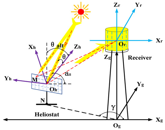
Figure 1.
A schematic diagram of the heliostat modeling.
- (1)
- Ignoring the influence of the small spacing of the mirror on the whole focusing process, the heliostat was regarded as a complete sphere.
- (2)
- All rays of the sun in the solar cone carry the same amount of energy.
The azimuth of an arbitrary number of heliostats in the field can be expressed as
where is the coordinate of the heliostat position in the ground coordinate system.
The vectorized representation of the incident ray (), reflected ray (), and the central normal of the heliostat () in the ground coordinate system
where is the solar altitude angle, is the solar azimuth angle, represents the rotational angle of the axis, which is perpendicular to the ground, and represents the pitch angle formed by pitching on the another axis.
The sun incidence angle () and the tracking rotation angle of the two axes of the heliostat can be obtained by
The vector of the solar incident ray in the heliostat coordinate system can be expressed as
The vector of the reflected ray in the heliostat coordinate system
where is the normal vector of any point in the heliostat coordinate system.
The vector of the reflected ray and point in the receiver coordinate system can be obtained by
Equation (12) is constructed from the reflection point and the direction vector of the reflected ray. Combined with Equation (13), which is the surface equation of the receiver, the coordinates of the intersection point can be solved.
The energy flux density can be obtained by counting the number of intersections in a certain region
where is the number of intersections in an area, is the number of incident rays, is the efficiency of the heliostat, is the area of the heliostat, and is the area of the reflection.
The heliostat field of a molten salt SPT plant is usually composed of thousands of the heliostats arranged in a circular shape, but there are no public data concerning the arrangement of a heliostat field in a power station at present. In order to achieve better simulation results, a heliostat field was optimized using SAM software in this paper. The arrangement of the heliostat field is shown in Figure 2. There were 5273 heliostats of 100 m2. The weather parameters, the heliostat coordinates and the structural parameters of the heliostat were taken as input parameters, and the actual working state of the heliostat was simulated.
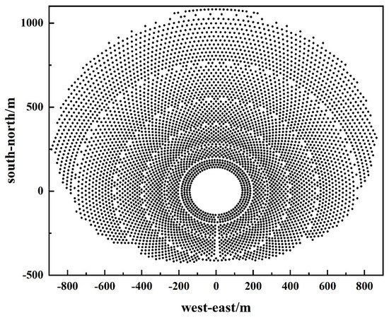
Figure 2.
The layout of the heliostat field.
2.2. Model of the Receiver
The external molten salt receiver was composed of 16 tube panels with two flow paths, and solar salt (60% NaNO3 and 40% KNO3) was used as the heat-absorbing working fluid. The molten salt enters the receiver from the north side of the tower, flows through the four tube panels and crosses the two paths to exchange heat, making the temperature uniform, and then flows into the remaining tube panels. The flow path of the molten salt and the heat transfer process of the tube panel are shown in Figure 3.
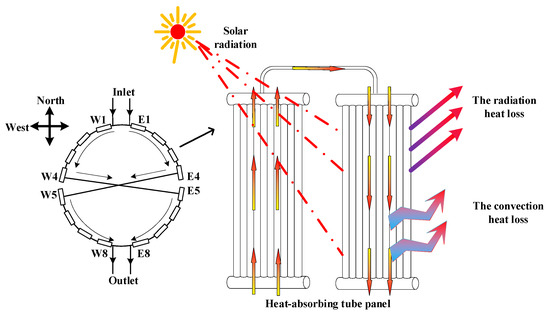
Figure 3.
The flow path of the molten salt and the heat transfer process of the tube panel.
The structural parameters of the external molten salt receiver were taken from the 50 MW SPT plant in Delingha, China, as shown in Table 1. A dynamic mathematical model for the flow and heat transfer of a single tube panel of the receiver was established using the modular modeling method. The assumptions and simplifications of the model were as follows:

Table 1.
Parameters of the molten salt receiver and collector field.
- (1)
- The flow in the tube was one-dimensional and unidirectional.
- (2)
- The variation in the potential energy and kinetic energy of the molten salt flow in the tube was ignored.
The radiant energy of the sun received by the surface of the receiver
Energy conservation of the tube panel
Energy conservation of the molten salt
Mass conservation of the molten salt
The heat absorption of the molten salt
The Nusselt number is based on an empirical formula [17]
where is the Darcy friction coefficient, which can be calculated with the Filonenko formula [18]
The Reynolds and Prandtl numbers of the molten salt can be expressed as
The convection heat loss
Comprehensive convective heat transfer coefficient [19]
The natural convection heat transfer coefficient between the heat-absorbing tube panel and the surrounding air [20]
Considering the installation height of external molten salt receiver is large, there is no shelter in the high altitude, the wind level is higher, air and tube panel forced convection occurs. The forced convection heat transfer coefficient is calculated according to the forced convection heat transfer of the air flow across the cylinder [21],
The radiation heat loss.
According to the Stefan–Boltzmann law, the radiant heat transfer between the tube panel and the environment is calculated as
where is the emissivity of the metal surface. The surface coating was Pyromark, and 0.95 was chosen here [22]. is the Boltzmann constant, 5.67 × 10⁻⁸ W/(m2∙K).
The mathematical model was solved using the Euler algorithm. The molten salt outlet temperature and tube wall temperature can be calculated with Equation (32).
where is the calculation step, and is the integral time step size.
2.3. Model Validation
The model’s parameters were set in accordance with the parameters of the Solar Two power plant, and the test data on 5 March 1999 were compared [23]. The data comparisons are shown in Table 2. The simulation results of the molten salt outlet temperature were for 558.1 ℃ and the operational data for 565.0 °C when the flow rate was 79 kg/s; thus, the relative error was 1.22%. The relative error of the molten salt outlet temperature was 0.53% when the flow rate was reduced to 36 kg/s. The error of the thermal efficiency was lower than 1.6%; therefore, the reliability of the model was validated.
Table 2.
The comparison of the simulation results and test data.
3. Results with Analysis
3.1. The Dynamic Characteristics of the Energy Flux Density
The dynamic simulation model of the integrated heat-collecting and heat-absorbing by the 50 MW molten salt SPT plant was run on the STAR-90 simulation platform. The 2021 equinox day (i.e., March 20) was selected as a typical day and the operational conditions on this date were simulated. The observed meteorological data for the station location were taken as the input parameters. The meteorological data were from Delingha, China. The change in the DNI data on the vernal equinox is displayed in Figure 4. A three-dimensional diagram of the energy flux distribution on the surface of the receiver at each typical moment is shown in Figure 5. The plane of the x-axis and y-axis in the diagram represents the eight tube panels on the west side of the molten salt receiver.
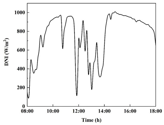
Figure 4.
DNI on the vernal equinox.
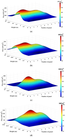
Figure 5.
Energy flux distribution on the surface of the receiver at each typical moment: (a) energy flux distribution at 12:00; (b) energy flux distribution at 14:00; (c) energy flux distribution at 16:00; (d) energy flux distribution at 18:00.
The figures indicate that the energy flux distribution on the surface of the tube panel was very uneven. The energy flux of a single tube panel was high in the middle and low on both sides; that is, the position of the entrance and exit of the tube panel was low and the position of the middle was high. The energy flux density on a single tube panel was in a Gaussian distribution. This distribution mode was influenced by the central point focusing mode adopted in the heliostat field. The variation of the DNI had a direct effect on the total energy absorbed by the receiver, and the energy flux on the surface of the receiver had a positive correlation with the DNI. Moreover, the maximum energy flux at each specific time appeared in sequence on the W1 to W4 panels. Over time, the highest point moved toward the tube panel behind the flow path. The energy flux on the surface of the last four tube panels (from W5 to W8) decreased in turn.
According to the distribution of the energy flux density, the wall temperature of the tube panel and molten salt temperature were calculated, and the temperature distribution at a specific time is shown in Figure 6. It can be seen that the distribution curve of the wall temperature on a single tube panel was similar to that of the energy flux along the axial direction, both rising at first and then decreasing. This shows that the wall temperature at the inlet and outlet of the tube panel was lower, but the wall temperature at the middle was higher. It also demonstrates the consistency of the temperature and energy flux changes. The nonuniform distribution of the energy flux made the highest wall temperature appear in the middle of the panel, which was also the reason for the tube wall temperature fluctuation. The temperature of the molten salt increased gradually with the flow process in the receiver. The temperature of the molten salt at the outlet of the receiver was the highest because of the cascade arrangement of each panel and the superposition effect of the temperature. The difference between the molten salt temperature and the tube wall temperature decreased gradually along the flow direction. The maximum temperature difference was at the first panel, and the minimum temperature difference was at the eighth panel. At 16:00, the DNI was the largest of the four time points; thus, the wall temperature and molten salt outlet temperature were also the highest. At this time, the maximum temperature difference at the first panel was 66.8 ℃ in the middle of the panel, and the minimum temperature difference at the eighth panel was 25.3 °C. It is shown that the first tube panel was easily affected by a large temperature difference, while the eighth panel was easily affected by a high temperature. More attention should be paid in both of these locations in the operation of the receiver. At 14:00 and 18:00, the DNI decreased seriously, and the molten salt outlet temperature was 383.1 and 388.2 °C, respectively, which was much lower than the rated outlet temperature of 565 °C. At this time, the thermal storage system will play a role to ensure the operation of the power plant system. Overall, the energy flux density varied with the change in the DNI and had a certain rule with the change in the time.
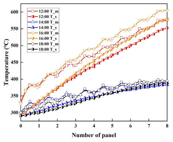
Figure 6.
The temperature distribution at a specific time.
3.2. The Dynamic Characteristics of the Receiver under Variable Operating Conditions
The operation of the external molten salt receiver was affected by many factors, including the DNI, flow rate and molten salt inlet temperature. Based on the operation of the 50 MW photothermal coupled dynamic model under a 100% load condition, the three factors mentioned above were taken as step disturbance variables, the dynamic characteristics of the molten salt receiver under disturbance were studied and the outlet temperature changes of the molten salt and tube wall were observed. The main parameters of the receiver under full load conditions are shown in Table 3.
Table 3.
The main parameters of the receiver under full load conditions.
3.2.1. DNI Disturbance
In the actual operation of the SPT plant, the solar radiation reaching the heliostat field will change sharply due to the weather, thus causing a large fluctuation in the molten salt outlet temperature of the receiver. The rapid change in temperature seriously affects its safe operation. In order to improve the operational safety, the dynamic response characteristics of the receiver under variable operating conditions were investigated, and a DNI step disturbance simulation was carried out.
The receiver operated under the rated operating condition, and the first disturbance was applied after 15 s, which makes the DNI step decreased by 30%, from 900 to 630 W/m2. The other quantities remained constant, and the second disturbance was applied after 60 s and the DNI increased by 10% to 720 W/m2; the changes in the molten salt outlet temperature and tube wall temperature are shown in Figure 7. When the temperature was stable, the temperature of the tube wall decreased by 28.1 °C, and the molten salt outlet temperature decreased by 25.3 °C; this shows that the tube wall temperature was more susceptible to disturbance. The temperature response time was less than 10 s when the disturbance occurs.
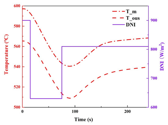
Figure 7.
The results of the DNI disturbance.
3.2.2. The Flow Rate Disturbance
For the sake of keeping the molten salt outlet temperature constant, the flow rate of the molten salt entering the receiver was adjusted in real time, according to the variation of the solar radiation. Therefore, as the main regulation of the receiver, it is very important to master the rule of the molten salt flow rate, which affects the temperature of the receiver. Therefore, a step disturbance simulation of the molten salt flow rate was carried out.
The receiver operated under 100% operating conditions, and the molten salt flow rate was reduced by 15% from 680 to 578 t/h at 15 s. After the disturbance, which lasted for 60 s, the flow rate increased by 5% to 612 t/h and kept constant until the temperature was stable. The results of the flow rate disturbance are shown in Figure 8. It can be seen that there was a negative correlation between the temperature and flow rate, because at a constant input energy, the flow rate decreased, while the unit volume of the molten salt absorbed more heat. Before the second disturbance was applied, the molten salt outlet temperature reached 598.1 °C, which seriously overheated and affected the safe operation of the receiver. The temperature was also less than 10 s to complete the response to the flow rate disturbance.
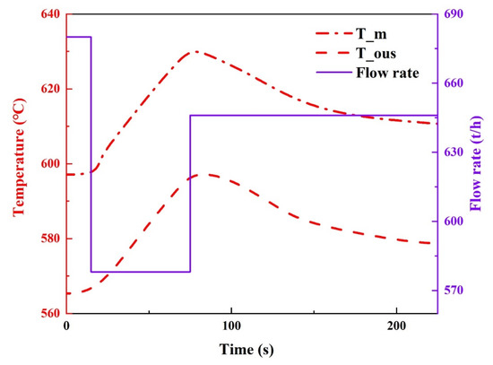
Figure 8.
The results of the flow rate disturbance.
3.2.3. Inlet Temperature Disturbance
Salt tanks are equipped in large-scale SPT plants to ensure continuous operation. However, a large volume salt tank results in the uneven distribution of the molten salt temperature. The molten salt inlet temperature is difficult to maintain at a constant value. Therefore, it is necessary to study the dynamic characteristics of the receiver by a step disturbance simulation of the molten salt inlet temperature.
The molten salt inlet temperature increased from 290 to 320 °C at 15 s and then decreases to 300 °C at 150 s. The results of the disturbance test are shown in Figure 9. It can be seen from the diagram that the response of the molten salt outlet temperature to the step disturbance of the molten salt inlet temperature was obviously delayed, and the temperature changed approximately 35 s after the first disturbance was applied. At the end of the disturbance, the molten salt inlet temperature increased by 10 °C, while the molten salt outlet temperature increased by 5.5 °C. It was obvious that the change in the outlet temperature was less than the inlet temperature. In addition, the change in the wall temperature was only 4.2 °C. This shows that the effect of the molten salt inlet temperature on the molten salt outlet temperature was mainly reflected in the longer response time.
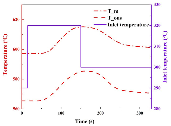
Figure 9.
The results of the inlet temperature disturbance.
The results of the step disturbance simulations show that the changes in the DNI, molten salt mass flow rate and molten salt inlet temperature had different effects on the molten salt outlet temperature and tube wall temperature. The variation in the DNI and flow rate directly affected the molten salt outlet temperature and caused it to fluctuate in a large range, while the influence of the molten salt inlet temperature was weaker. The response time of the molten salt outlet temperature to the inlet temperature was significantly longer, and the variation degree of the outlet temperature was less than the fluctuation range of the inlet temperature. Therefore, the wide range of the changes in the DNI should be closely watched, as well as the accurate control of the flow rate changes in the process of operation. The long response time of the molten salt outlet temperature to the inlet temperature should also be considered in the formulation of the control strategy.
4. Conclusions
In this paper, a heliostat field model and an external molten salt receiver model were established, and a 50 MW integrated photothermal dynamic model was developed using the design parameters of a practical SPT plant. The nonuniform and time-varying characteristics of the surface energy flux of the receiver were studied by simulating the operation of an actual power plant on the vernal equinox day. The dynamic characteristics of the molten salt receiver under different operating conditions were investigated using the step disturbance simulations of the DNI, molten salt flow rate and molten salt inlet temperature. The obtained results are helpful for the safe operation, as well as the formulation of a control strategy, of an SPT plant. The conclusions are as follows:
- (1)
- There was a strong positive correlation between the overall change trend in the nonuniform energy flux density on the surface of the external receiver and the change in the DNI. From 12:00 to 18:00, the maximum energy flux density on the surface of the tube panel moved from the first panel on the west side gradually to the fourth, and the energy flux density of the last four panels decreased in sequence.
- (2)
- The energy flux distribution on a single tube panel was high in the middle and low at the inlet and outlet. In addition, the temperature distribution on the tube wall was basically consistent with the energy flux distribution along the axial direction, which increased first and then decreases. The temperature difference between the inner and outer walls of the first tube panel was the largest, and the molten salt temperature of the eighth panel was the highest.
- (3)
- The step disturbances in the DNI and molten salt flow rate had a more direct influence on the change in the molten salt outlet temperature and tube wall temperature than that of the molten salt inlet temperature disturbance. However, the response time of the molten salt inlet temperature disturbance was longer than that of the former two. Therefore, DNI monitoring and accurate control of the molten salt flow rate should be paid more attention during the operation of an SPT plant. At the same time, the influence of the long response time characteristics of the molten salt inlet temperature on the formulation of the control strategy should be considered.
Author Contributions
Conceptualization, E.X.; investigation, H.H.; data curation, H.H.; writing—original draft preparation, H.H.; writing—review and editing, L.S. and Q.Z.; supervision, Q.H.; funding acquisition, E.X. All authors have read and agreed to the published version of the manuscript.
Funding
This work was funded by the National Natural Science Foundation of China (Grant No. 51976058).
Institutional Review Board Statement
Not applicable.
Informed Consent Statement
Not applicable.
Data Availability Statement
Not applicable.
Conflicts of Interest
The authors declare that they have no known competing financial interests or personal relationships that may affect the work reported in this paper.
Nomenclature
| a | thermal diffusivity, m2/s |
| A | solar collecting area, m2 |
| C | specific heat capacity, kJ/(kg·k) |
| d | inner diameter of the receiver, m |
| fD | friction coefficient |
| Gr | Grashof number |
| h | heat transfer coefficient, kW/m2·K |
| Hr | height of the receiver, m |
| Hor | installation height, m |
| M | mass, kg |
| Nu | Nusselt number |
| Pr | Prandtl number calculated based on the fluid temperature |
| Q | heat, kW |
| R | radius of the heat receiver, m |
| Re | Reynolds number |
| t | temperature, °C |
| Δt | temperature difference between the air and tube wall, K |
| T_m | tube wall temperature, K |
| T_ous | molten salt outlet temperature, K |
| u | velocity, m/s |
| V | volume, m3 |
| G | mass flow rate, kg/s |
| αv | expansion coefficient of air, K−1 |
| direction vector | |
| azimuth of the heliostat, rad | |
| emissivity | |
| sun incidence angle, rad | |
| azimuth angle of the rotating shaft, rad | |
| pitching angle of the rotating shaft, rad | |
| thermal conductivity, kW/m·K | |
| dynamic viscosity, N·s/m2 | |
| kinematic viscosity, m2/s | |
| density, kg/m3 | |
| Stefan–Boltzmann constant | |
| time, s | |
| energy flux density, kW/m2 | |
| a | air |
| abs | energy absorbed |
| amb | ambient |
| fc | forced convection |
| g | ground coordinate system |
| h | heliostat coordinate system |
| in | inlet/incident |
| lc | convective heat loss |
| lr | radiative heat loss |
| m | metal tube wall |
| nc | natural convection |
| nor | normal |
| ou | outlet |
| r | receiver coordinate system |
| ref | reflected ray |
| s | molten salt |
| DNI | direct normal irradiation |
| SPT | solar power tower |
References
- Ma, X.-J.; Chen, R.-M.; Su, H. Driving Factors and Decoupling Analysis on Industrial Energy Consumption in China. Stat. Inf. Forum 2021, 36, 70–81. [Google Scholar]
- Li, L.; Lin, J.; Wu, N.; Xie, S.; Meng, C.; Zheng, Y.; Wang, X.; Zhao, Y. Review and Outlook on the International Renewable Energy Development. Energy Built Environ. 2020, 3, 139–157. [Google Scholar] [CrossRef]
- Mekhilef, S.; Saidur, R.; Safari, A. A review on solar energy use in industries. Renew. Sustain. Energy Rev. 2011, 15, 1777–1790. [Google Scholar] [CrossRef]
- He, Y.-L.; Qiu, Y.; Wang, K.; Yuan, F.; Wang, W.-Q.; Li, M.-J.; Guo, J.-Q. Perspective of concentrating solar power. Energy 2020, 198, 117373. [Google Scholar] [CrossRef]
- Yu, H.; Duan, J.; Du, W.; Xue, S.; Sun, J. China’s energy storage industry: Develop status, existing problems and countermeasures. Renew. Sustain. Energy Rev. 2017, 71, 767–784. [Google Scholar] [CrossRef]
- Du, B.-C.; He, Y.-L.; Zheng, Z.-J.; Cheng, Z.-D. Analysis of thermal stress and fatigue fracture for the solar tower molten salt receiver. Appl. Therm. Eng. 2016, 99, 741–750. [Google Scholar] [CrossRef]
- Qiu, Y.; He, Y.-L.; Li, P.-W. A comprehensive model for analysis of real-time optical performance of a solar power tower with a multi-tube cavity receiver. Appl. Energy 2017, 185, 589–603. [Google Scholar] [CrossRef]
- Cruz, N.C.; Redondo, J.L.; Álvarez, J.D.; Berenguel, M.; Ortigosa, P.M. A parallel Teaching–Learning-Based Optimization procedure for automatic heliostat aiming. J. Supercomput. 2016, 73, 591–606. [Google Scholar] [CrossRef]
- Xu, L.; Stein, W.; Kim, J.-S.; Too, Y.C.S.; Guo, M.; Wang, Z. Transient numerical model for the thermal performance of the solar receiver. Appl. Therm. Eng. 2018, 141, 1035–1047. [Google Scholar] [CrossRef]
- Sánchez-González, A.; Santana, D. Solar flux distribution on central receivers: A projection method from analytic function. Renew. Energy 2015, 74, 576–587. [Google Scholar] [CrossRef]
- Ho, C.K.; Khalsa, S.S. A Photographic Flux Mapping Method for Concentrating Solar Collectors and Receivers. J. Sol. Energy Eng. 2012, 134, 041004. [Google Scholar] [CrossRef]
- Besarati, S.M.; Yogi Goswami, D.; Stefanakos, E.K. Optimal heliostat aiming strategy for uniform distribution of heat flux on the receiver of a solar power tower plant. Energy Convers. Manag. 2014, 84, 234–243. [Google Scholar] [CrossRef]
- Yu, Q.; Wang, Z.; Xu, E. Analysis and improvement of solar flux distribution inside a cavity receiver based on multi-focal points of heliostat field. Appl. Energy 2014, 136, 417–430. [Google Scholar] [CrossRef]
- Sun, F.-H.; Wang, Z.-F.; Guo, M.-H.; Liang, W.-F. An automatic alignment system of heliostat based on the method of track axis reference dislocation. J. Sol. Energy 2016, 37, 877–883. [Google Scholar]
- Hu, Y.; Xu, Z.; Zhou, C.; Du, J.; Yao, Y. Design and performance analysis of a multi-reflection heliostat field in solar power tower system. Renew. Energy 2020, 160, 498–512. [Google Scholar] [CrossRef]
- Victor, G.; Kypros, M.; Clotilde, C. Heliostat fields with a balanced mirror density. Sol. Energy 2022, 243, 336–347. [Google Scholar]
- Gnielinski, V. New Equations For Heat And Mass-Transfer In Turbulent Pipe And Channel Flow. Int. Chem. Eng. 1976, 16, 359–368. [Google Scholar]
- Colebrook, C. Turbulent flow in pipes with particular reference to the transition region between smooth and rough pipe laws. Ice 1939, 11, 133–156. [Google Scholar] [CrossRef]
- Winter, C.-J.; Sizmann, R.L.; Vant-Hull, L.L. Solar Power Plants: Fundamentals, Technology, Systems, Economics; Springer: Berlin, Germany, 1991. [Google Scholar]
- Siebers, D.L.; Kraabel, K.J. Estimating Convective Energy Losses from Solar Central Receivers; Sandia National Laboratories: Albuquerque, NM, USA, 1984. [Google Scholar]
- Wagner, M. Simulation and Predictive Performance Modeling of Utility-Scale Central Receiver System Power Plants; University of Wisconsin-Madison: Madison, WI, USA, 2008. [Google Scholar]
- Zhang, Q.; Cao, D.; Ge, Z.; Du, X. Response characteristics of external receiver for concentrated solar power to disturbance during operation. Appl. Energy 2020, 278, 115709. [Google Scholar] [CrossRef]
- Bradshaw, R.W.; Dawson, D.B.; Rosa, D.L.; Gilbert, R.; Goods, S.H.; Hale, M.J.; Jacobs, P.; Jones, S.A.; Kolb, G.J.; Pacheco, J.E.; et al. Final Test and Evaluation Results from the Solar Two Project; National Renewable Energy Laboratory (NREL): Golden, CO, USA, 2002. [Google Scholar]
Disclaimer/Publisher’s Note: The statements, opinions and data contained in all publications are solely those of the individual author(s) and contributor(s) and not of MDPI and/or the editor(s). MDPI and/or the editor(s) disclaim responsibility for any injury to people or property resulting from any ideas, methods, instructions or products referred to in the content. |
© 2023 by the authors. Licensee MDPI, Basel, Switzerland. This article is an open access article distributed under the terms and conditions of the Creative Commons Attribution (CC BY) license (https://creativecommons.org/licenses/by/4.0/).