AWEbox: An Optimal Control Framework for Single- and Multi-Aircraft Airborne Wind Energy Systems

Abstract

In this paper, we present AWEbox, a Python toolbox for modeling and optimal control of multi-aircraft systems for airborne wind energy (AWE). AWEbox provides an implementation of optimization-friendly multi-aircraft AWE dynamics for a wide range of system architectures and modeling options. It automatically formulates typical AWE optimal control problems based on these models, and finds a numerical solution in a reliable and efficient fashion. To obtain a high level of reliability and efficiency, the toolbox implements different homotopy methods for initial guess refinement. The first type of method produces a feasible initial guess from an analytic initial guess based on user-provided parameters. The second type implements a warm-start procedure for parametric sweeps. We investigate the software performance in two different case studies. In the first case study, we solve a single-aircraft reference problem for a large number of different initial guesses. The homotopy methods reduce the expected computation time by a factor of 1.7 and the peak computation time by a factor of eight, compared to when no homotopy is applied. Overall, the CPU timings are competitive with the timings reported in the literature. When the user initialization draws on expert a priori knowledge, homotopies do not increase expected performance, but the peak CPU time is still reduced by a factor of 5.5. In the second case study, a power curve for a dual-aircraft lift-mode AWE system is computed using the two different homotopy types for initial guess refinement. On average, the second homotopy type, which is tailored for parametric sweeps, outperforms the first type in terms of CPU time by a factor of three. In conclusion, AWEbox provides an open-source implementation of efficient and reliable optimal control methods that both control experts and non-expert AWE developers can benefit from.

1. Introduction

Airborne wind energy (AWE) is a renewable energy technology that aims at harvesting strong and steady high altitude winds that cannot be reached using conventional wind technology, at a fraction of the material resources [1]. It is based on the principle of one or more tethered autonomous aircraft flying fast crosswind maneuvers. In the majority of AWE concepts, electricity is either produced by onboard turbines on the aircraft and conducted to a ground station through the tether (drag-mode), or in a periodic fashion by reeling out the tether at a high tension to drive a winch at the ground station, and reeling back in at low tension, so as to achieve a net positive energy output over one period (lift-mode). Although there exist many other interesting AWE concepts, e.g., those based on tethered rotorcrafts [2,3], we will limit the scope of this paper to rigid-wing lift- and drag-mode systems. The reader is referred to [4,5] for a recent and comprehensive overview of the different technologies.

The principle of AWE was first investigated in 1980 by Miles Loyd, who derived an upper limit for the power that could be produced by a crosswind AWE system [6]. Since then, in the past two decades, in particular, AWE has gained increasing interest from both academia and industry, leading to significant technological progress and many small- to medium-scale prototypes, the largest of which was based on a 26 m wing span aircraft [7]. While AWE developers are considering a multitude of different designs, most systems are based on a single-aircraft setup. At this moment, AWE technology is still in a pre-commercial stage, with some companies taking the first steps towards market entry [8]. One of the central unresolved challenges for AWE developers is achieving techno-economic performance at utility scale, i.e., designing systems that produce large amounts of electricity at low cost.

Multi-aircraft systems have been proposed and investigated in the literature as a more efficient and cheaper way of producing utility-scale electricity [9,10,11,12]. In a multi-aircraft AWE system, two or more tethered aircraft fly tight crosswind maneuvres around a shared main tether, thereby minimizing the latter’s crosswind motion and hence, the associated dissipation losses due to aerodynamic drag. These systems can be up to twice as efficient as their single-aircraft counterparts [10], while having superior, modular, upscaling properties [12], intrinsically smooth power output profiles [13], and higher potential power densities in farm configurations [14]. As a consequence of the increased system complexity, this system class has thus far only been investigated in simulation studies.

A crucial condition for the performance of both single- and multi-aircraft systems is finding power-efficient flight paths that satisfy flight envelope constraints and airframe load limits. This is not only necessary for path planning purposes but also for, e.g., offline performance prediction, design optimization, and control strategy design. Optimal control is an evidently suitable path planning technique for AWE, given its natural ability to handle unstable, nonlinear, constrained systems with multiple in- and outputs. In the past decade, it has become an established method in the field, leading to various applications ranging from performance assessment studies [15], over model predictive control [16], and system identification [17], to flight path planning for a real-world soft-kite system [18]. We refer the reader to [19] for a complete overview of applications.

Despite its obvious advantages, optimal control comes with its own challenges: the dependence on an accurate model; the computational burden associated with finding a numerical solution; and a rather complex implementation that heavily relies on expert knowledge. In case an accurate model is unavailable, it is possible to resort to model-free, adaptive techniques, such as extremum seeking (ES) [20] or iterative learning control (ILC) [21]. However, in [22], a validated reference model was proposed for a lift-mode, rigid-wing single-aircraft system. While identifying the parameters of such a model is a complicated and time-consuming task [17,23], this shows that deriving a physical model that fits the measurements very well is, in principle, possible. In the following, we will focus on the two other challenges mentioned above.

In order to increase computational efficiency, a general model structure based on non-minimal coordinates was proposed in [24], resulting in smooth dynamic equations of low symbolic complexity. Additionally, since the system nonlinearity gives rise to highly non-convex optimization problems, a feasible initial guess is typically needed for fast and reliable convergence of Newton-type optimization solvers. Such an initial guess is, in many cases, not available a priori. Therefore, a homotopy procedure was proposed that produces a close-to-optimal, feasible initial guess based on a generic, naive one [25]. Combined with a direct-collocation-based transcription method, this led to reported computation times of below one minute for a representative power cycle of a lift-mode AWE system with a six-degree-of-freedom aircraft model [26]. Another homotopy variant was investigated in [27] to efficiently compute drag-mode power cycles for large-scale wind data.

In this work, we consider direct collocation approaches with local support, i.e., using several subintervals with each its own, small set of collocation points. However, for smooth trajectories, it is often more efficient to apply a global support approach [28], using Fourier interpolating polynomials for periodic solutions. This approach has been proposed for drag-mode AWE systems in [29], using a frequency-domain formulation. For lift-mode systems, the optimal solution contains sharp transitions between the reel-out and reel-in phases, and it is a priori unclear which method will be more efficient. For future comparison, the global-support approach can be easily implemented using the collocation framework of the proposed toolbox.

While many open-source AWE control and simulation frameworks exist for single-aircraft models [30,31], and even for multi-aircraft models [32], there are only a few available open-source implementations of optimization methods tailored for AWE. The Matlab library MegAWES [20] provides an implementation of a megawatt-class system model and of a power optimization algorithm based on ES. The Optimal Control Library OpenOCL [33] provides a user-friendly Matlab interface for formulating and solving OCPs, which can be linked to the optimization-friendly lift-mode model implemented in the framework OpenAWE [34]. However, this framework does not offer homotopy-based initial guess refinement or multi-aircraft models.

In this paper, we present AWEbox, an open-source Python framework for modeling and optimal control of single- and multi-aircraft AWE systems. The contributions of the software package can be summarized as follows:

• Usability: the user specifies only high-level modeling and optimization parameters. AWEbox implements optimization-friendly system dynamics for single- and multi-aircraft systems, for various system architectures and combinations of model options. It automatically formulates typical AWE optimization problems and implements and interfaces the algorithms needed to compute a numerical solution efficiently.
• Reliability: AWEbox increases reliability by efficiently computing a feasible OCP initial guess via homotopy methods, based on an analytic initial guess defined using a small number of user input parameters. The framework also implements an algorithm to efficiently and reliably perform parameter sweeps.
• Extensibility: within the baseline non-minimal-coordinates structure, users can add new or alternative modeling components (e.g., wind model, aerodynamics, etc.) in a straightforward fashion. The homotopy procedure for initial guess refinement can be extended in a modular fashion so that new model components can be introduced without affecting reliability.

AWEbox is freely available and open-source under the GNU LGPLv3, which allows use in proprietary software. The toolbox heavily builds on lower-level open-source software packages such as CasADi [35], a framework for algorithmic differentiation and optimization, and the nonlinear program (NLP) solver IPOPT [36].

The remainder of this paper is structured as follows. Section 2 discusses the multi-aircraft modeling procedure, while Section 3 gives an overview of the optimization ingredients used to formulate and numerically solve periodic AWE optimal control problems. Section 4 then outlines the software implementation details. Section 5 presents two case studies that highlight the efficiency and reliability of the implementation, as well as its multi-aircraft capability. Section 6 draws conclusions based on these results and makes suggestions for further research.

2. AWE Modeling for Optimal Control

In this section, we define the multi-aircraft topologies considered in AWEbox. We outline the optimization-friendly AWE model structure for six-degrees-of-freedom (6DOF) aircraft dynamics as described in [22] and the extensions made for the multi-aircraft case [12,37]. The different additional model components presented in this section are not novel per se but rather collected and integrated from our own previous work as well as from the literature.

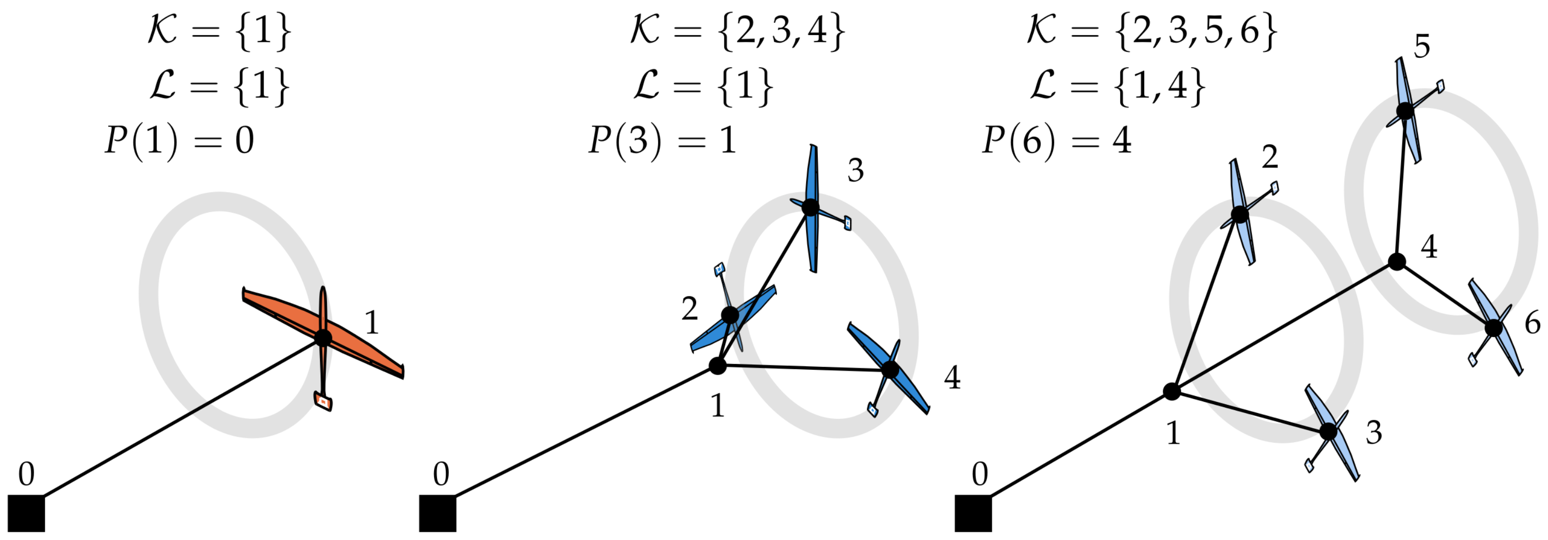
2.1. Topology

We consider any tree-structured multi-aircraft topology as previously introduced in [12]. Each tree is described by a set of nodes $\mathcal{N}$, where each node $n\in \mathcal{N}$ represents the end-point of a tether. All tethers in the tree are assumed to be rigid and straight, which is a reasonable assumption if tether tension is high compared to gravity and tether drag. Note that this assumption allows for a very good agreement with experimental flight data of the single-aircraft system in [22]. In case a higher accuracy is desired, the topology can be readily extended by discretizing the tethers into finite elements, adding a node for each segment, as proposed in [10].

Some of the nodes $k\in \mathcal{K}$ correspond to aircraft nodes, while other nodes $l\in \mathcal{L}$ are layer nodes, with $\mathcal{L}:=\mathcal{N}\backslash \mathcal{K}$ if $\left|\mathcal{N}\right|>1$ and $\mathcal{L}:=\mathcal{N}$ in the single-aircraft case. The parent map $P\left(n\right)$ uniquely defines the interlinkage between nodes, and the children map $C\left(n\right):=\{\overline{n}\in \mathcal{N}|P\left(\overline{n}\right)=n\}$ returns the set of nodes with parent n. Figure 1 illustrates the proposed notation for some typical examples.

2.2. System Dynamics and Variables

The considered topologies require a multi-body modeling approach that should exhibit certain optimization-friendly properties. For one, the dynamics should have a low symbolic complexity to allow for fast repeated numerical evaluation, in particular of its sensitivities. Second, model nonlinearity should be kept low in order to enable fast and reliable use of Newton-type optimization techniques. Third, the model should avoid singularities that might be visited by and crash the optimization algorithm.

In [24], the efficacy of a non-minimal coordinates modeling approach to describe the translational and rotational dynamics of multiple interlinked aircraft is demonstrated. In this approach, each node is considered as a separate rigid body and linked by algebraic constraints. The aircraft orientation is parametrized in a non-singular fashion using the direction cosine matrix (DCM).

The resulting multi-body models are of reasonable complexity and nonlinearity but result in model equations in the form of index-3 DAEs. This representation does not allow for the deployment of classical integration methods within the optimal control problem [38]. Therefore an index-reduction technique is applied, which involves time-differentiation of the algebraic constraints. The resulting model equations for both lift- and drag-mode AWE systems are summarized by the following index-1 DAE:

$$\mathbf{F}(\dot{\mathbf{x}}\left(t\right),\mathbf{x}\left(t\right),\mathbf{u}\left(t\right),\mathbf{z}\left(t\right),\mathbf{\theta },\mathbf{p})=0,$$

(1)

with associated consistency conditions $\mathbf{C}\left(\mathbf{x}\right(t\left)\right)=0,\forall t\in \mathbb{R}$.

To define the differential state vector $\mathbf{x}$ for both lift- and drag-mode systems, we first define the basic multi-aircraft state

$${\mathbf{x}}^{\mathrm{base}}:=(\mathbf{q},\dot{\mathbf{q}},\mathbf{R},\mathbf{\omega },\mathbf{\delta }).$$

(2)

This state vector firstly contains $\mathbf{q}$ and $\dot{\mathbf{q}}$ that are concatenations of the node positions ${\mathbf{q}}_n\in {\mathbb{R}}^3$ and velocities ${\dot{\mathbf{q}}}_n\in {\mathbb{R}}^3$ respectively, $\forall n\in \mathcal{N}$. These are followed by the states specific to aircraft nodes, namely $\mathbf{R},\mathbf{\omega },\mathbf{\delta }$, which are concatenations of all ${\mathbf{R}}_k,{\mathbf{\omega }}_k,{\mathbf{\delta }}_k,\forall k\in \mathcal{K}$. The DCMs ${\mathbf{R}}_k:=[{\widehat{\mathbf{e}}}_{1,k},{\widehat{\mathbf{e}}}_{2,k},{\widehat{\mathbf{e}}}_{3,k}]\in {\mathbb{R}}^{3\times 3}$ contain the chord-wise, span-wise and upwards unit vectors of the aircraft body frames, expressed in the inertial frame $\{{\mathbf{e}}_{\mathrm{x}},{\mathbf{e}}_{\mathrm{y}},{\mathbf{e}}_{\mathrm{z}}\}$. All DCMs should be orthonormal, i.e., they are constrained to evolve on the 3D manifold defined by

$${\mathbf{c}}_{\mathrm{R},k}:=P_{\mathrm{ut}}({\mathbf{R}}_k^{\top }{\mathbf{R}}_k-I)=0,$$

(3)

where the operator $P_{\mathrm{ut}}$ is used to select the six upper triangular elements of a matrix. The aircraft angular velocities ${\mathbf{\omega }}_k\in {\mathbb{R}}^3$ are given in the body frame. The surface deflections ${\mathbf{\delta }}_k=[{\delta }_{\mathrm{a},k},{\delta }_{\mathrm{e},k},{\delta }_{\mathrm{r},k}]\in {\mathbb{R}}^3$ of aileron, elevator, and rudder, respectively, give control over the aircraft aerodynamics.

The lift- and drag-mode state vector can now be defined as

$$\begin{array}{cc}\hfill {\mathbf{x}}^{\mathrm{lift}}:=({\mathbf{x}}^{\mathrm{base}},l_{\mathrm{t}},{\dot{l}}_{\mathrm{t}})& \mathrm{and}{\mathbf{x}}^{\mathrm{drag}}:=({\mathbf{x}}^{\mathrm{base}},\mathbf{\kappa }),\hfill \end{array}$$

(4)

where the tether length $l_{\mathrm{t}}\in \mathbb{R}$ and speed ${\dot{l}}_{\mathrm{t}}\in \mathbb{R}$ describe the main tether reel-in and -out evolution. The variable $\mathbf{\kappa }$ is the concatenation of all ${\kappa }_k\in \mathbb{R},\forall k\in \mathcal{K}$, which represent the onboard turbine drag coefficients.

The controls

$$\begin{array}{cc}\hfill {\mathbf{u}}^{\mathrm{lift}}:=(\dot{\mathbf{\delta }},{\ddot{l}}_{\mathrm{t}})& \mathrm{and}{\mathbf{u}}^{\mathrm{drag}}:=(\dot{\mathbf{\delta }},\dot{\mathbf{\kappa }})\hfill \end{array}$$

(5)

are given by the concatenation of all aircraft surface deflection rates ${\dot{\mathbf{\delta }}}_k\in {\mathbb{R}}^3$ and by either the tether acceleration ${\ddot{l}}_{\mathrm{t}}\in \mathbb{R}$ or the concatenation of the turbine drag coefficient derivatives ${\dot{\kappa }}_k\in \mathbb{R}$.

The algebraic variables $\mathbf{z}:=\mathbf{\lambda }$ describe the concatenation of all Lagrange multipliers ${\lambda }_n\in \mathbb{R}$ related to the tether constraints that restrict the position of each node $n\in \mathcal{N}$ to evolve on a 2D manifold defined by

$$c_n:=\frac{1}{2}\left(\Delta \mathbf{q}{\left(n\right)}^{\top }\Delta \mathbf{q}\left(n\right)-l_n^2\right)=0,$$

(6)

where

$$\Delta \mathbf{q}\left(n\right):=\left\{\begin{array}{cc}{\mathbf{q}}_n-{\mathbf{q}}_{P\left(n\right)},\hfill & \mathrm{if}n\notin \mathcal{K},\hfill \\ {\mathbf{q}}_n+{\mathbf{R}}_n{\mathbf{r}}_{\mathrm{t}}-{\mathbf{q}}_{P\left(n\right)},\hfill & \mathrm{if}n\in \mathcal{K}.\hfill \end{array}\right.$$

(7)

In these constraints, ${\mathbf{r}}_{\mathrm{t}}$ is the tether attachment point described in the aircraft frame. The variable $l_n$ describes the tether length associated with node n and is defined together with the tether diameter $d_n$ as

$$(l_n,d_n):=\left\{\begin{array}{cc}(l_{\mathrm{t}},d_{\mathrm{t}}),\hfill & \mathrm{if}n=1,\hfill \\ (l_{\mathrm{s}},d_{\mathrm{s}}),\hfill & \mathrm{if}n\in \mathcal{K}\backslash \left\{1\right\},\hfill \\ (l_{\mathrm{i}},d_{\mathrm{i}}),\hfill & \mathrm{if}n\in \mathcal{L}\backslash \left\{1\right\},\hfill \end{array}\right.$$

(8)

with $l_{\mathrm{s}}$ and $d_{\mathrm{s}}$ the length and diameter of the secondary tethers and $l_{\mathrm{i}}$ and $d_{\mathrm{i}}$ those of the layer-linking tethers in stacked multi-aircraft configurations.

The ground station is located at the origin of the inertial frame, such that ${\mathbf{q}}_0:=\mathbf{0}$.

The variables $\mathbf{\theta }$ represent variable system parameters that can be optimized over. In the general stacked multi-aircraft case, they are defined as

$${\mathbf{\theta }}^{\mathrm{lift}}:=(l_{\mathrm{s}},\mathit{d})\mathrm{and}{\mathbf{\theta }}^{\mathrm{drag}}:=(l_{\mathrm{t}},l_{\mathrm{s}},\mathit{d})$$

(9)

where $\mathit{d}:=(d_{\mathrm{t}},d_{\mathrm{s}},d_{\mathrm{i}})$.

The constant parameters $\mathbf{p}$ allow the dynamics to be evaluated for varying model parameters, such as aircraft wing span, wind model parameters, etc. The system parameter values used in the numerical experiments in this paper are listed in Appendix A,

Table A1. System parameters.

Description	Parameter	Value	Units
Aircraft mass	$m_{\mathrm{K}}$	$3.6800·{10}^1$	kg
Moment of inertia	$J_{\mathrm{K},x}$	$2.5000·{10}^1$	kg·m${}^2$
Moment of inertia	$J_{\mathrm{K},y}$	$3.2000·{10}^1$	kg·m${}^2$
Moment of inertia	$J_{\mathrm{K},z}$	$5.6000·{10}^1$	kg·m${}^2$
Moment of inertia	$J_{\mathrm{K}z,xz}$	$4.7000·{10}^{-1}$	kg·m${}^2$
Wing span	b	$5.5000·{10}^0$	m
Wing chord	c	$5.5000·{10}^{-1}$	m
Wing area	S	$3.0000·{10}^0$	m${}^2$
Tether drag coefficient	$C_{\mathrm{D},\mathrm{t}}$	$1.2000·{10}^0$	-
Tether density	${\rho }_{\mathrm{t}}$	$1.4642·{10}^3$	kg·m${}^{-3}$
Tether Baumgarte constant	${\kappa }_{\mathrm{t}}$	$1.0000·{10}^0$	-
Tether attachment point	$r_{\mathrm{t},\mathrm{x}},r_{\mathrm{t},\mathrm{y}},r_{\mathrm{t},\mathrm{z}}$	$0.0000·{10}^0$	m
DCM Baumgarte constant	${\kappa }_{\mathrm{R}}$	$1.0000·{10}^0$	-
Wind friction coefficient	$c_{\mathrm{f}}$	$1.5000·{10}^{-1}$	-
Reference height	$z_{\mathrm{ref}}$	$1.0000·{10}^2$	m
Sea level temperature	$T_0$	$2.8820·{10}^2$	K
Temperature lapse rate	$T_{\mathrm{L}}$	$6.5000·{10}^{-3}$	K·m${}^{-1}$
Sea level air density	${\rho }_0$	$1.2250·{10}^0$	kg·m${}^{-3}$
Tether safety factor	$f_{\mathrm{s}}$	$3.0000·{10}^0$	-
Anticollision safety factor	$f_{\mathrm{b}}$	$4.0000·{10}^0$	-

.

2.3. Lagrangian Dynamics

The system dynamics (1) can be derived in accordance with the Lagrangian approach proposed in [24]. The system Lagrangian is defined as

$$L:=T-V-{\mathit{\lambda }}^{\top }\mathit{c},$$

(10)

with $\mathit{c}$ the concatenation of all tether constraints $c_n$ for all $n\in \mathcal{N}$ and with the kinetic energy T and potential energy V defined as

$$\begin{array}{cc}\hfill T:=& \sum _{k\in \mathcal{K}}{T}_{\mathrm{K},k}+\sum _{n\in \mathcal{N}}{T}_{\mathrm{t},n}\hfill \end{array}$$

(11)

$$\begin{array}{cc}\hfill V:=& \sum _{k\in \mathcal{K}}{m}_{\mathrm{K}}g{\mathbf{q}}_k^{\top }{\mathbf{e}}_{\mathrm{z}}+\sum _{n\in \mathcal{N}}\frac{1}{2}{m}_{\mathrm{t},n}g{({\mathbf{q}}_n-{\mathbf{q}}_{P\left(n\right)})}^{\top }{\mathbf{e}}_{\mathrm{z}}.\hfill \end{array}$$

(12)

Here, $m_{\mathrm{K}}$ is the aircraft mass, and the tether mass $m_{\mathrm{t},n}:={\rho }_{\mathrm{t}}{l}_n\frac{\pi d_n^2}{4}$, with ${\rho }_{\mathrm{t}}$ the tether material density, and g is the gravitational acceleration. The kinetic energy related to the aircraft $T_{\mathrm{K},k}$ and to the tethers $T_{\mathrm{t},n}$ [39] are given by

$$\begin{array}{cc}\hfill T_{\mathrm{K},k}:=& \frac{1}{2}{m}_{\mathrm{K}}{\dot{\mathbf{q}}}_k^{\top }{\dot{\mathbf{q}}}_k+\frac{1}{2}{\mathbf{\omega }}_k^{\top }{J}_{\mathrm{K}}{\mathbf{\omega }}_k,\hfill \end{array}$$

(13)

$$\begin{array}{cc}\hfill T_{\mathrm{t},n}:=& \frac{1}{6}{m}_{\mathrm{t},n}({\dot{\mathbf{q}}}_n^{\top }{\dot{\mathbf{q}}}_n+{\dot{\mathbf{q}}}_{P\left(n\right)}^{\top }{\dot{\mathbf{q}}}_{P\left(n\right)}+{\dot{\mathbf{q}}}_n^{\top }{\dot{\mathbf{q}}}_{P\left(n\right)}),\hfill \end{array}$$

(14)

with $J_{\mathrm{K}}$ the aircraft moment of inertia and with the tether velocity at the ground station given by

$$\begin{array}{c}\hfill {\dot{\mathbf{q}}}_0:={\dot{\mathbf{q}}}_1^{\top }{\mathbf{e}}_{\mathrm{t}}\mathrm{with}{\mathbf{e}}_{\mathrm{t}}:=\frac{{\mathbf{q}}_1}{l_{\mathrm{t}}}.\end{array}$$

(15)

Note that for a drag-mode system with constant tether length, this implies that ${\dot{\mathbf{q}}}_0=0$.

With the system Lagrangian defined, the translational dynamics read:

$$\frac{\mathrm{d}}{\mathrm{d}t}\frac{\partial L}{\partial \dot{\mathbf{q}}}-\frac{\partial L}{\partial \mathbf{q}}=\mathbf{F}+{\mathbf{F}}_{\mathrm{corr}}$$

(16)

with $\mathbf{F}$ the concatenation of the external forces ${\mathbf{F}}_n$ exerted on each of the nodes. The term ${\mathbf{F}}_{\mathrm{corr}}$ is a Lagrangian momentum correction term for open systems:

$${\mathbf{F}}_{\mathrm{corr}}:=\sum _{n\in \mathcal{N}}\frac{\mathrm{d}{m}_n}{\mathrm{d}t}{\dot{\mathbf{q}}}_n^{\top }\frac{\partial {\dot{\mathbf{q}}}_n}{\partial \dot{\mathbf{q}}}.$$

(17)

This term is non-zero for lift-mode systems since tether mass and energy are entering and leaving the system due to the reeling motion.

The rotational dynamics are projected on a 3D manifold in the aircraft body frame [24] so as to read:

$$J_{\mathrm{K}}\frac{\mathrm{d}{\mathbf{\omega }}_k}{\mathrm{d}t}+{\mathbf{\omega }}_k\times J_{\mathrm{K}}{\mathbf{\omega }}_k+2U\left({\mathbf{R}}_k^{\top }{\nabla }_{{\mathbf{R}}_k}{\mathbf{\lambda }}^{\top }\mathbf{c}\right)={\mathbf{M}}_k,\forall k\in \mathcal{K},$$

(18)

with ${\mathbf{M}}_k$ the aerodynamic moment exerted on the aircraft and with U the “unskew" operator, i.e., $U\left(\mathtt{skew}\right(\mathbf{a}\left)\right)=\mathbf{a}$, as defined in [24].

Next to the dynamic equations, also the holonomic constraints $\mathit{c}=0$ need to be enforced. Since these constraints do not explicitly depend on the generalized accelerations $\ddot{\mathbf{q}}$ or on the algebraic variables $\mathit{\lambda }$, it is not possible to numerically integrate the resulting dynamic equations with standard algorithms. Therefore an index reduction is performed by differentiating $\mathit{c}$ twice with respect to time. Note that $\ddot{\mathit{c}}$ depends on $\ddot{\mathbf{q}}$.

Because of the index reduction, as well as the over-parametrization of the rotational degrees-of-freedom, the consistency conditions $\mathbf{C}\left(\mathbf{x}\right):=(\mathbf{c},\dot{\mathbf{c}},{\mathbf{c}}_{\mathrm{R}})=0$ must be enforced at an arbitrary time point in the trajectory. These quantities are called invariants, since their value is preserved by the dynamics. System invariants, when not dealt with carefully, can lead to failure of the Linear Independence Constraint Qualification (LICQ) in the context of periodic optimal control. Performing Baumgarte stabilization on the invariants is an effective way to avoid this issue, while simultaneously ensuring that $\mathbf{C}\left(\mathbf{x}\right)=0$ is satisfied over the entire time period [40]. Therefore the tether constraint dynamics are augmented with the following Baumgarte stabilization scheme:

$$\ddot{\mathit{c}}+2{\kappa }_{\mathrm{t}}\dot{\mathit{c}}+{\kappa }_{\mathrm{t}}^2\mathit{c}=0,$$

(19)

with ${\kappa }_{\mathrm{t}}$ a Baumgarte tuning parameter [41].

2.4. System Kinematics

The system dynamics also describe the following trivial kinematics. First, as explained in the previous section, the rotational kinematics are augmented with a Baumgarte-type stabilization on the orthogonality conditions [42]:

$$\frac{\mathrm{d}{\mathbf{R}}_k}{\mathrm{d}t}={\mathbf{R}}_k\left(\frac{{\kappa }_{\mathrm{R}}}{2}(I-{\mathbf{R}}_k^{\top }{\mathbf{R}}_k)+\mathtt{skew}\left({\mathbf{\omega }}_k\right)\right),$$

(20)

with ${\kappa }_{\mathrm{R}}$ another tuning parameter. The remaining kinematics

$$\begin{array}{c}\hfill \frac{\mathrm{d}}{\mathrm{d}t}(\mathbf{q},\mathbf{\delta })=(\dot{\mathbf{q}},\dot{\mathbf{\delta }}),\frac{\mathrm{d}}{\mathrm{d}t}(l_{\mathrm{t}},{\dot{l}}_{\mathrm{t}})=({\dot{l}}_{\mathrm{t}},{\ddot{l}}_{\mathrm{t}})(lift-mode),\frac{\mathrm{d}}{\mathrm{d}t}\mathbf{\kappa }=\dot{\mathbf{\kappa }}(drag-mode),\end{array}$$

(21)

together with (16)–(20) then complete the system dynamics summarized by (1). The remaining modeling effort now focuses on the generalized forces $\mathbf{F}$ and moments $\mathbf{M}$.

2.5. Wind and Atmosphere Model

AWE systems typically operate at altitudes of several hundreds of meters, and the altitude variation within a typical power cycle is of the same order of magnitude [15]. In particular, the multi-aircraft variant, unhindered by the drag losses caused by main tether cross-wind motion, can theoretically operate at arbitrarily high altitudes, wherever the wind power density is highest [10,12]. Therefore, a wind model is needed that accounts for the varying wind power availability with altitude. Within the community, it is common to use one of the following approximations:

(a)

Logarithmic profile: A logarithmic model [43] is typically used as a very simple wind shear approximation. Assuming steady, laminar flow, the logarithmic model provides us with the following expression for the freestream wind velocity ${\mathbf{u}}_{\infty }\left(z\right)$:

$${\mathbf{u}}_{\infty }\left(z\right):=u_{\mathrm{ref}}\frac{log\frac{z}{z_0}}{log\frac{z_{\mathrm{ref}}}{z_0}}{\mathbf{e}}_{\mathrm{x}},$$

(22)

which, in this model, is assumed to be aligned with the x-axis in the inertial frame. Here, $u_{\mathrm{ref}}$ is the reference wind speed that is measured at an altitude $z_{\mathrm{ref}}$, whereas $z_0$ is the surface roughness length, which depends on local terrain characteristics.

(b)

Power-law profile: Another frequent approximation is given by the power law:

$${\mathbf{u}}_{\infty }\left(z\right):=u_{\mathrm{ref}}{\left(\frac{z}{z_{\mathrm{ref}}}\right)}^{c_{\mathrm{f}}}{\mathbf{e}}_{\mathrm{x}},$$

(23)

where $c_{\mathrm{f}}$ is a ground surface friction coefficient. We will use this model in the numerical experiments in this paper, in accordance with case studies in [15,22].

(c)

2D wind data interpolation: The disadvantage of the logarithmic and power-law models is that they are only useful for representing long-term average wind conditions. Realistic wind profiles come in a wide variety of shapes and are subject to strong short-term (hourly, diurnal, seasonal) changes. Furthermore, the approximation accuracy typically breaks down at altitudes relevant to AWE systems [44] while failing to account for the effect of vertical atmospheric stability. Hence, for accurate optimal-control-based power curve and capacity factor estimation, it is often necessary to generate a more detailed but still differentiable wind model based on highly spatially resolved wind speed measurements. To achieve this, we adopt the approach presented in [27,45]. We assume a wind profile that is represented by discrete 2D wind measurements ${\mathbf{u}}_{\mathrm{m},1},\dots ,{\mathbf{u}}_{\mathrm{m},n_{\mathrm{lag}}}\in {\mathbb{R}}^2$. These measurements correspond to a set of altitudes $z_1,\dots ,z_{n_{\mathrm{lag}}}$. We can then create a smooth wind model to approximate the measured wind profile, by creating an interpolating function based on Lagrange polynomials:

$$\mathcal{W}(z,\mathbf{\zeta }):=\sum _{i=1}^{n_{\mathrm{lag}}}\left({\mathbf{\zeta }}_i·\prod _{\begin{array}{c}k=1\\ k\ne i\end{array}}^{n_{\mathrm{lag}}}\frac{z-z_k}{z_i-z_k}\right),$$

(24)

with $\mathbf{\zeta }$ the concatenation of the polynomial coefficients ${\mathbf{\zeta }}_i\in {\mathbb{R}}^2$ obtained by solving the following optimization problem

$${\mathbf{\zeta }}^{*}:=\underset{\mathbf{\zeta }}{\arg \min } \frac{1}{2}\sum _{i=1}^{n_{\mathrm{lag}}}{\parallel \mathcal{W}(z_i,\mathbf{\zeta })-{\mathbf{u}}_{\mathrm{m},i}\parallel }^2+k{∥\frac{{\mathrm{d}}^2\mathcal{W}}{\mathrm{d}{z}^2}(z_i,\mathbf{\zeta })∥}^2.$$

(25)

The cost function is tuned with weight k so that ${\mathbf{\zeta }}_i^{*}\approx {\mathbf{u}}_{\mathrm{m},i}$, $\forall i=1\dots n_{\mathrm{lag}}$, while preventing overfitting via the penalization of the second derivative of the interpolating polynomials. The smooth and differentiable wind model is then given by

$${\mathbf{u}}_{\infty }\left(z\right):=(\mathcal{W}(z,{\mathbf{\zeta }}^{*}),0).$$

(26)

Wind power availability is linear in the air density, and the atmospheric density drop is non-negligible in the altitudes relevant to AWE. Therefore the density variation with altitude $\rho \left(z\right)$ is modeled according to the international standard atmosphere model [43]:

$$\rho \left(z\right):={\rho }_0{\left(\frac{T_0-T_{\mathrm{L}}z}{T_0}\right)}^{\frac{g}{T_{\mathrm{L}}R}-1},$$

(27)

where R is the universal gas constant. The parameters $T_0$ and ${\rho }_0$ are the temperature and air density at sea level, and $T_{\mathrm{L}}$ is the temperature lapse rate.

Alternatively, the user can provide a set of density data points at different altitudes. The continuous density profile $\rho \left(z\right)$ is then constructed similar to the wind profile with smoothed Lagrange polynomials, cfr. (24) and (25).

2.6. Aerodynamic Model

The apparent wind at each aircraft node $k\in \mathcal{K}$ is defined as

$${\mathbf{u}}_{\mathrm{a},k}:={\mathbf{u}}_{\infty }\left({\mathbf{q}}_k^{\top }{\mathbf{e}}_{\mathrm{z}}\right)-{\dot{\mathbf{q}}}_k.$$

(28)

We then define the dynamic pressure as $q_k:=\frac{1}{2}\rho \left({\mathbf{q}}_k^{\top }{\mathbf{e}}_{\mathrm{z}}\right){\parallel {\mathbf{u}}_{\mathrm{a},k}\parallel }^2$. The aerodynamic forces (in the inertial frame) and moments (in the body frame) on the aircraft wings are then given using

$$\begin{array}{c}\hfill {\mathbf{F}}_{\mathrm{A},k}:=q_{k}S{\mathbf{R}}_k{\mathbf{C}}_{\mathrm{F},k}\mathrm{and}{\mathbf{M}}_{\mathrm{A},k}:=q_{k}S\left[\begin{array}{ccc}b& 0& 0\\ 0& c& 0\\ 0& 0& b\end{array}\right]{\mathbf{C}}_{\mathrm{M},k}.\end{array}$$

(29)

with S the aircraft aerodynamic surface and with the aerodynamic coefficients ${\mathbf{C}}_{\mathrm{F},k}:=(C_{\mathrm{X},k},C_{\mathrm{Y},k},C_{\mathrm{Z},k})$ and ${\mathbf{C}}_{\mathrm{M},k}:=(C_{\mathrm{l},k},C_{\mathrm{m},k},C_{\mathrm{n},k})$, which are a function of the angles of attack ${\alpha }_k$ and side-slip angles ${\beta }_k$, given by the small-angle approximations

$$\begin{array}{c}\hfill {\alpha }_k:=\frac{{\widehat{\mathbf{e}}}_{3,k}^{\top }{\mathbf{u}}_{\mathrm{a},k}}{{\widehat{\mathbf{e}}}_{1,k}^{\top }{\mathbf{u}}_{\mathrm{a},k}}\mathrm{and}\beta :=\frac{{\widehat{\mathbf{e}}}_{2,k}^{\top }{\mathbf{u}}_{\mathrm{a},k}}{{\widehat{\mathbf{e}}}_{1,k}^{\top }{\mathbf{u}}_{\mathrm{a},k}}.\end{array}$$

(30)

The force and moment coefficients ${\mathbf{C}}_{\diamond ,k}$ (with $\diamond \in \left\{\mathrm{F},\mathrm{M}\right\}$) read as

$$\begin{array}{c}\hfill {\mathbf{C}}_{\diamond ,k}:={\mathbf{C}}_{\diamond ,0}\left({\alpha }_k\right)+{\mathbf{C}}_{\diamond ,\beta }\left({\alpha }_k\right){\beta }_k+{\mathbf{C}}_{\diamond ,\mathbf{\omega }}\left({\alpha }_k\right)\left[\begin{array}{ccc}b& 0& 0\\ 0& c& 0\\ 0& 0& b\end{array}\right]\frac{{\mathbf{\omega }}_k}{2\parallel {\mathbf{u}}_{\mathrm{a},k}\parallel }+{\mathbf{C}}_{\diamond ,\mathbf{\delta }}\left({\alpha }_k\right){\delta }_k\end{array}$$

(31)

The dependence of these coefficients on ${\alpha }_k$ is approximated by second-order polynomials of the form:

$$C_{\diamond ,\circ }\left(\alpha \right):=\left[\begin{array}{ccc}{c}_{\diamond ,\circ ,2}& c_{\diamond ,\circ ,1}& c_{\diamond ,\circ ,0}\end{array}\right]\left[\begin{array}{c}{\alpha }^2\\ \alpha \\ 1\end{array}\right]$$

(32)

with the values of the coefficients $c_{\diamond ,\circ ,i}$ used in this study given in Table 2 in [22].

The tether drag is modeled as follows. Consider the infinitesimal tether drag force $\mathrm{d}{\mathbf{F}}_{\mathrm{td},n}\left(s\right):={\mathbf{F}}_{\mathrm{td},n}\left(s\right)\mathrm{d}s$ on an infinitesimal segment $l_n\mathrm{d}s$, for $s\in \left[0,1\right]$, with:

$${\mathbf{F}}_{\mathrm{td},n}\left(s\right):=\frac{1}{2}\rho \left({\mathbf{q}}_{\mathrm{t},n}{\left(s\right)}^{\top }{\mathbf{e}}_{\mathrm{z}}\right)C_{\mathrm{D},\mathrm{t}}{d}_n{l}_n\parallel {\mathbf{u}}_{\mathrm{t},n}\left(s\right)\parallel {\mathbf{u}}_{\mathrm{t},n}\left(s\right),$$

(33)

with $C_{\mathrm{D},\mathrm{t}}$ the tether drag coefficient, and where the segment position and apparent wind speed are given by

$$\begin{array}{cc}\hfill {\mathbf{q}}_{\mathrm{t},n}\left(s\right):=& s{\mathbf{q}}_{P\left(n\right)}+(1-s){\mathbf{q}}_n\hfill \end{array}$$

(34)

$$\begin{array}{cc}\hfill {\mathbf{u}}_{\mathrm{t},n}\left(s\right):=& {\mathbf{u}}_{\infty }\left({\mathbf{q}}_{\mathrm{t},n}{\left(s\right)}^{\top }{\mathbf{e}}_{\mathrm{z}}\right)-{\dot{\mathbf{q}}}_{\mathrm{t},n}\left(s\right).\hfill \end{array}$$

(35)

It is shown in [39,46] that the total drag force can be exactly distributed into contributions on node n and on its parent node $P\left(n\right)$, so as to read

$$\begin{array}{c}\hfill {\mathbf{F}}_{\mathrm{td},n}^1:={\int }_0^{1}s{\mathbf{F}}_{\mathrm{td},n}\left(s\right)\mathrm{d}s\mathrm{and}{\mathbf{F}}_{\mathrm{td},n}^0:={\int }_0^1(1-s){\mathbf{F}}_{\mathrm{td},n}\left(s\right)\mathrm{d}s\end{array}$$

(36)

respectively. In order to be able to numerically evaluate the tether drag, the integrals in (36) are discretized using the midpoint rule. Typically, a number of $M_{\mathrm{td}}=5$ integration intervals is sufficiently accurate.

The generalized forces can now be defined for each node as

$$\begin{array}{c}\hfill {\mathbf{F}}_n^{★}:=\left\{\begin{array}{cc}{\mathbf{F}}_{\mathrm{A},n}+{\mathbf{F}}_{\mathrm{td},n}^1\hfill & \mathrm{if}n\in \mathcal{K}\wedge (★=\mathrm{lift})\hfill \\ {\mathbf{F}}_{\mathrm{A},n}+{\mathbf{F}}_{\mathrm{td},n}^1+{\mathbf{F}}_{\mathrm{turb},k}\hfill & \mathrm{if}n\in \mathcal{K}\wedge (★=\mathrm{drag})\hfill \\ {\mathbf{F}}_{\mathrm{td},n}^1+{\displaystyle \sum _{c\in C\left(n\right)}}{\mathbf{F}}_{\mathrm{t},c}^0\hfill & \mathrm{if}n\in \mathcal{N}\backslash \mathcal{K}\hfill \end{array}\right.\end{array}$$

(37)

and the generalized moments are given by the aerodynamic moments, i.e., ${\mathbf{M}}_k:={\mathbf{M}}_{\mathrm{A},k}$, $\forall k\in \mathcal{K}$. In the drag-mode case, also the braking force of the onboard turbines is acting on the aircraft:

$${\mathbf{F}}_{\mathrm{turb},k}:={\kappa }_k\parallel {\mathbf{u}}_{\mathrm{a},k}\parallel {\mathbf{u}}_{\mathrm{a},k}.$$

(38)

Note that the tether pulling force and moment exerted on the aircraft are implicitly modeled in the constraint-based dynamics (16) and (18) and should not be considered as part of the generalized forces.

2.7. Power Output

For lift-mode systems, the generated power is the product of the main tether force with the tether speed. The pulling force using a tether n experienced at node n is given by the expression ${\mathbf{F}}_{\mathrm{t},n}:=-{\lambda }_n{\nabla }_{{\mathbf{q}}_n}{c}_n$. Note that a positive multiplier corresponds to a positive pulling force. The power transferred through tether n is then given by $P_{\mathrm{t},n}:={\mathbf{F}}_{\mathrm{t},n}^{\top }{\dot{\mathbf{q}}}_n.$ For the main tether, this expression can be simplified to $P_{\mathrm{t},1}:=-{\lambda }_1{l}_{\mathrm{t}}{\dot{l}}_{\mathrm{t}}$. The mechanical power that arrives at the ground station is given by $P^{\mathrm{lift}}:=-P_{\mathrm{t},1}$.

In drag-mode systems, electrical power is generated by the onboard turbines and transferred to the ground station through the tethers. Each aircraft $k\in \mathcal{K}$ generates an amount of electrical power $P_{\mathrm{turb},k}:={\eta }_{\mathrm{turb}}{\kappa }_k{\parallel {\mathbf{u}}_{\mathrm{a},k}\parallel }^3$, with ${\eta }_{\mathrm{turb}}$ the onboard turbine efficiency. Note that for the case of power consumption, i.e., $\kappa <0$, the efficiency needs to be inverted. This can be implemented using the logistic function, as proposed in [29]. The total power output generated by the drag-mode system is then given by $P^{\mathrm{drag}}:={\displaystyle \sum _{k\in \mathcal{K}}}{P}_{\mathrm{turb},k}$.

3. Optimization Ingredients

In this section, we discuss all the necessary ingredients to formulate, discretize, and reliably solve power optimization problems for the system model described in the previous section. We state the periodic optimal control problem formulation in continuous time, and we discuss common system constraints. We explain the transcription method to convert the problem into an NLP, and we summarize the interior-point solution strategy used by IPOPT to solve it. Then we describe how the initial guess is constructed, and how it can be refined using two different homotopy methods that are tailored for interior-point NLP solvers. Finally, we discuss a third homotopy method that is tailored to perform parameter sweeps with interior-point NLP solvers.

3.1. Problem Formulation for Periodic Orbits

The main goal of the toolbox is to facilitate automated computation of dynamically feasible, power-optimal periodic orbits for both lift- and drag-mode systems while satisfying a set of relevant system constraints. In order to achieve this, we formulate a periodic optimal control problem of a free time period T, which has the distinctive property that the system state at the initial and final time of the OCP time horizon can be chosen freely by the solver but must be equal. Given that some key system parameters $\mathbf{\theta }$, such as the tether diameters and lengths, have a huge impact on the system power output and the optimal flight trajectories, they are included as optimization variables as well.

Let the optimization variables be defined as $\mathbf{w}:=\left(\mathbf{x}\right(·),\mathbf{u}(·),\mathbf{z}(·),\mathbf{\theta },T)$. Then we can compute a power-optimal state and control trajectories and a corresponding system design $\mathbf{\theta }$ for given parameters $\mathbf{p}$ by solving the following continuous-time optimization problem:

$$\underset{\mathbf{w}}{\min } \frac{1}{T}\underset{0}{\overset{T}{\int }}l(\mathbf{x}\left(t\right),\mathbf{u}\left(t\right),\mathbf{z}\left(t\right))\mathrm{d}t$$

(39a)

$$\mathrm{s}.\mathrm{t}. \mathbf{F}(\dot{\mathbf{x}}\left(t\right),\mathbf{x}\left(t\right),\mathbf{u}\left(t\right),\mathbf{z}\left(t\right),\mathbf{\theta },\mathbf{p})=0,\forall t\in [0,T]$$

(39b)

$$\hspace{1em} \mathbf{h}(\dot{\mathbf{x}}\left(t\right),\mathbf{x}\left(t\right),\mathbf{u}\left(t\right),\mathbf{z}\left(t\right),\mathbf{\theta },\mathbf{p})\le 0,\forall t\in [0,T]$$

(39c)

$$\mathbf{x}\left(0\right)-\mathbf{x}\left(T\right)=0$$

(39d)

$$\psi \left(\mathbf{x}\right(0\left)\right)=0.$$

(39e)

The Lagrange cost term is given by the sum of the negative power output and a penalty on the controls in order to mitigate actuator fatigue, as well as on the side slip angle and the angular accelerations in order to avoid aerodynamic side forces and aggressive maneuvers:

$$l(\mathbf{x}\left(t\right),\mathbf{u}\left(t\right),\mathbf{z}\left(t\right)):=-P\left(t\right)+\widehat{w}{\left(t\right)}^{\top }\mathbf{W}\widehat{w}\left(t\right),$$

(40)

with $\widehat{w}\left(t\right):=(\mathbf{u}\left(t\right),\mathbf{\beta }\left(t\right),\dot{\mathbf{\omega }}\left(t\right))$ and $\mathbf{W}$ a constant diagonal weighting matrix. The variables $\mathbf{\beta }$ and $\dot{\mathbf{\omega }}$ are the vertical concatenations of the side slip angles ${\beta }_k$ and angular accelerations ${\dot{\mathbf{\omega }}}_k$, $\forall k\in \mathcal{K}$. Proper tuning of the weighting matrix $\mathbf{W}$ is necessary to achieve fast convergence of the optimization algorithm as well as to obtain a locally unique solution. We refer the reader to the open-source code for the weighting factors used in the numerical experiments in this study.

The function $\psi :{\mathbb{R}}^{n_{\mathrm{x}}}\to \mathbb{R}$ is used to impose a technical constraint that removes the phase invariance inherent to periodic OCPs. For lift- and drag-mode systems, this function is different and reads as either

$${\psi }^{\mathrm{lift}}\left({\mathbf{x}}^{\mathrm{lift}}\left(0\right)\right):={\dot{l}}_{\mathrm{t}}\left(0\right)\stackrel{!}{=}0\mathrm{or}{\psi }^{\mathrm{drag}}\left({\mathbf{x}}^{\mathrm{drag}}\left(0\right)\right):={\dot{\mathbf{q}}}_1{\left(0\right)}^{\top }{\mathbf{e}}_{\mathrm{y}}\stackrel{!}{=}0.$$

(41)

The inequality constraints $\mathbf{h}$ are discussed in the following section.

Note that the consistency conditions $\mathbf{C}\left(\mathbf{x}\right(t\left)\right)=0$ are not enforced at any given time within the time horizon of the OCP. In combination with the periodicity constraint (39d), this would lead to LICQ deficiency for all feasible trajectories. There exist several technical solutions for this issue [40]. In the dynamic correction approach chosen here, Baumgarte stabilization is applied to the consistency conditions in the system dynamics, as previously mentioned in Section 2.3. Therefore the dynamics of $\mathbf{C}$ are exponentially stable, and since with the value of periodicity, it holds that $\mathbf{C}\left(\mathbf{x}\right(0\left)\right)=\mathbf{C}\left(\mathbf{x}\right(T\left)\right)$, the only feasible periodic state trajectories are those where $\mathbf{C}\left(\mathbf{x}\right(t\left)\right)=0$, $\forall t\in [0,T]$.

3.2. System Constraints

A particular feature of OCP (39) is that it has an economic cost function, which is not lower bounded, as opposed to tracking cost functions [47]. OCPs with an economic cost function tend to have extreme solutions in the absence of constraints. In the context of AWE power optimization, it is, therefore, crucial to impose constraints that avoid a violation of the flight envelope, and that preserve the structural integrity of the airframe and the tether.

The flight envelope consists of upper and lower bounds on the angle-of-attack $\mathbf{\alpha }$ (to avoid stall) and the side-slip angle $\mathbf{\beta }$ (to avoid additional drag and preserve model validity) for all aircraft in the system. Additionally, the stress in the tethers should not exceed the yield strength with a certain safety factor $f_{\mathrm{s}}$:

$${\sigma }_n:=f_{\mathrm{s}}\frac{4\parallel {\mathbf{F}}_{\mathrm{t},n}\parallel }{\pi d_n^2}\le {\sigma }_{max},\forall n\in \mathcal{N}.$$

(42)

Here, the tether force magnitude can be simplified to $\parallel {\mathbf{F}}_{\mathrm{t},n}\parallel ={\lambda }_n{l}_n$, following the definition in Section 2.7. The aircraft orientation is also constrained in order to avoid collision of the airframe with the tether, which might occur during sharp turns in transition maneuvers:

$${({\mathbf{q}}_k-{\mathbf{q}}_{P\left(k\right)})}^{\top }{\widehat{\mathbf{e}}}_{3,k}\ge cos\left({\gamma }_{max}\right)l_k,\forall k\in \mathcal{K},$$

(43)

where ${\gamma }_{max}$ is the maximum angle between the tether vector and the upwards unit vector of the aircraft body frame, which should be set lower than at most $\pi /2$. In the multi-aircraft case, the following anti-collision constraints might be included:

$${\parallel {\mathbf{q}}_k-{\mathbf{q}}_m\parallel }_2\ge f_{\mathrm{b}}b,\forall k,m\in \mathcal{K},k\ne m,$$

(44)

where $f_{\mathrm{b}}$ is safety factor in multiples of the wing span b.

Along these nonlinear constraints, variable bounds are typically imposed on variables such as flight altitude, tether length, speed and acceleration, aircraft angular velocity, control surface deflections and their rates, etc. One pair of variable bounds that is crucial in the context of periodic optimal control are the bounds on the time period T. Since the OCP will be discretized in a discrete number of numerical integration intervals, the integration accuracy is variable along with T. Therefore, T should be bounded from above to guarantee an acceptable simulation accuracy. Also, by translating a priori knowledge on the optimal value of T into variable bounds, we narrow the search space and exclude many possible local solutions, which typically increases reliability and speeds up the convergence of the NLP solver.

3.3. Problem Transcription

The continuous-time OCP (39) has an infinite number of variables and constraints. Hence, we apply direct optimal control to transcribe the OCP to an NLP. We choose transcription by direct collocation, which is a fully simultaneous approach, where the numerical simulation variables are treated as variables in the optimization problem [26]. We choose this approach for the following reasons.

First, fully simultaneous optimal control is characterized by faster contraction rates of the Newton-type iterations compared to simultaneous and sequential optimal control, in particular for highly nonlinear and unstable systems [48]. Second, in the fully simultaneous case, the simulation problem is solved directly by the NLP solver, which is typically more robust than the rootfinder used in standard available numerical integrators. Finally, since OCP (39) is highly non-convex, the NLP solver benefits from computing the Newton step using exact Hessian information. The NLP Hessian becomes considerably cheaper to evaluate in the fully simultaneous approach.

Although the resulting direct collocation NLP is comparably large, it is also sparse. In combination with a sparsity-exploiting NLP solver, direct collocation is a highly efficient transcription method for the models presented in this paper.

In direct collocation, the time horizon is divided into N (usually equidistant) intervals described by $[t_i,t_{i+1}]$, where $0<t_0<t_1<\dots <t_N=T$. The control trajectory is parameterized as a piecewise constant function $\tilde{\mathbf{u}}\left(t\right):={\mathbf{u}}_i\mathrm{if}t\in [t_i,t_{i+1})$. The state trajectory is parametrized by piecewise polynomials of order $M+1$, i.e., $\tilde{\mathbf{x}}\left(t\right):={\tilde{\mathbf{x}}}_i\left(t\right)$ $\mathrm{if}t\in [t_i,t_{i+1})$, with

$${\tilde{\mathbf{x}}}_i\left(t\right):=\sum _{j=0}^M{\xi }_j\left(\tau \right){\mathbf{x}}_{i,j}^{\prime },$$

(45)

with the normalized time $\tau \frac{t-t_i}{\Delta t_i},\tau \in [0,1]$, with $\Delta t_i:=t_{i+1}-t_i$ and with the variables ${\mathbf{x}}_{i,j}^{\prime }$ placed at the time points $({\tau }_0,\mathbf{\tau })$, with $\mathbf{\tau }:=({\tau }_1,\dots ,{\tau }_M)$ and with ${\tau }_{0}0$. The Lagrange polynomials ${\xi }_j$ are uniquely defined by the choice of collocation grid points $\mathbf{\tau }$:

$${\xi }_j\left(\tau \right):=\prod _{\begin{array}{c}k=0\\ k\ne j\end{array}}^M\frac{{\tau }_k-\tau }{{\tau }_k-{\tau }_j}.$$

(46)

Note that it holds that ${\tilde{\mathbf{x}}}_i(t_i+\Delta t_i{\tau }_j)={\mathbf{x}}_{i,j}^{\prime }$. The state derivative is given by the derivative of the polynomials, i.e.,

$${\dot{\tilde{\mathbf{x}}}}_i\left(t\right):=\sum _{j=0}^M\frac{1}{\Delta t_i}\frac{\mathrm{d}{\xi }_j}{\mathrm{d}\tau }\left(\tau \right){\mathbf{x}}_{i,j}^{\prime }.$$

(47)

The algebraic variables are also discretized in each i’th time interval as ${\mathbf{z}}_{i,j}^{\prime }$, and allocated to the collocation points ${\tau }_1,\dots ,{\tau }_M$.

Let us now define ${\mathbf{x}}_i:={\mathbf{x}}_{i,0}^{\prime }$, ${\mathbf{X}}_i:=[{\mathbf{x}}_{i,1}^{\prime },\dots ,{\mathbf{x}}_{i,M}^{\prime }]$ and ${\mathbf{Z}}_i:=[{\mathbf{z}}_{i,1}^{\prime },\dots ,{\mathbf{z}}_{i,M}^{\prime }]$. Then, for given state vector ${\mathbf{x}}_i$ at the start of each interval, the collocation variables ${\mathbf{X}}_i$ and ${\mathbf{Z}}_i$ are uniquely determined by enforcing the system dynamics (1) at the grid points ${\tau }_1,\dots ,{\tau }_M$:

$${\mathbf{G}}_i({\mathbf{x}}_i,{\mathbf{u}}_i,{\mathbf{X}}_i,{\mathbf{Z}}_i,\mathbf{\theta },\mathbf{p},T):=\left[\begin{array}{c}\mathbf{F}\left({\dot{\tilde{\mathbf{x}}}}_i(t_i+\Delta t_i{\tau }_1),{\mathbf{x}}_{i,1}^{\prime },{\mathbf{u}}_i,{\mathbf{z}}_{i,1}^{\prime },\mathbf{\theta },\mathbf{p}\right)\\ \mathbf{F}\left({\dot{\tilde{\mathbf{x}}}}_i(t_i+\Delta t_i{\tau }_2),{\mathbf{x}}_{i,2}^{\prime },{\mathbf{u}}_i,{\mathbf{z}}_{i,2}^{\prime },\mathbf{\theta },\mathbf{p}\right)\\ ⋮\\ \mathbf{F}\left({\dot{\tilde{\mathbf{x}}}}_i(t_i+\Delta t_i{\tau }_M),{\mathbf{x}}_{i,M}^{\prime },{\mathbf{u}}_i,{\mathbf{z}}_{i,M}^{\prime },\mathbf{\theta },\mathbf{p}\right)\end{array}\right]=0.$$

(48)

The state transition from one interval node to the next is given by the equation

$${\mathbf{x}}_{i+1}=\mathbf{\varphi }({\mathbf{x}}_i,{\mathbf{X}}_i)\mathrm{with}\mathbf{\varphi }({\mathbf{x}}_i,{\mathbf{X}}_i):={\tilde{\mathbf{x}}}_i\left(t_{i+1}\right)=\sum _{j=0}^M{\xi }_j\left(1\right){\mathbf{x}}_{i,j}^{\prime }.$$

(49)

The system of Equation (48) corresponds to that of an implicit Runge–Kutta integration scheme, where the choice of collocation grid points $\mathbf{\tau }$ uniquely defines the Butcher-Tableau of the specific integration method. Here, we choose as collocation grid points the roots of Gauss–Radau polynomials, more specifically those corresponding to the Radau IIa integration scheme because of its high order accuracy and its excellent stability properties (A- and L-stability), which is particularly relevant for DAE systems [49].

Further, the inequality constraints are imposed on the interval nodes, and the Lagrange term in the cost function can be computed via a quadrature rule [26]:

$$\underset{t_i}{\overset{t_{i+1}}{\int }}l(\mathbf{x}\left(t\right),\mathbf{u}\left(t\right),\mathbf{z}\left(t\right)\mathrm{d}t\approx \Delta t_i\sum _{j=1}^M{b}_j^{\prime }·l({\mathbf{x}}_{i,j}^{\prime },{\mathbf{u}}_i,{\mathbf{z}}_{i,j}^{\prime }),$$

(50)

where the quadrature weights are given by

$$\left[\begin{array}{ccc}{b}_1^{\prime }& \dots & b_M^{\prime }\end{array}\right]:=\left[\begin{array}{ccc}{\xi }_1\left(1\right)& \dots & {\xi }_M\left(1\right)\end{array}\right]{\left[\begin{array}{ccc}\frac{\mathrm{d}{\xi }_1}{\mathrm{d}\tau }\left({\tau }_1\right)& \dots & \frac{\mathrm{d}{\xi }_M}{\mathrm{d}\tau }\left({\tau }_1\right)\\ ⋮& \ddots & ⋮\\ \frac{\mathrm{d}{\xi }_1}{\mathrm{d}\tau }\left({\tau }_M\right)& \dots & \frac{\mathrm{d}{\xi }_M}{\mathrm{d}\tau }\left({\tau }_M\right)\end{array}\right]}^{-1}.$$

(51)

The NLP resulting from discretizing the OCP (39) using direct collocation is then formulated as

$$\underset{\mathbf{w}}{\min } \frac{1}{T}\sum _{i=0}^{N-1}\Delta t_i\sum _{j=1}^M{b}_j^{\prime }·l({\mathbf{x}}_{i,j}^{\prime },{\mathbf{u}}_i,{\mathbf{z}}_{i,j}^{\prime })$$

(52a)

$$\mathrm{s}.\mathrm{t}.\hspace{1em}{\mathbf{x}}_{i+1}-\mathbf{\varphi }({\mathbf{x}}_i,{\mathbf{X}}_i)=0,\forall i=0,\dots ,N-1$$

(52b)

$${\mathbf{G}}_i({\mathbf{x}}_i,{\mathbf{u}}_i,{\mathbf{X}}_i,{\mathbf{Z}}_i,\mathbf{\theta },\mathbf{p},T)=0,\forall i=0,\dots ,N-1$$

(52c)

$$\mathbf{h}({\dot{\tilde{\mathbf{x}}}}_i(t_i+\Delta i{\tau }_M),{\mathbf{X}}_{i,M},{\mathbf{u}}_i,{\mathbf{Z}}_{i,M},\mathbf{\theta },\mathbf{p})\le 0,\forall i=0,\dots ,N-1$$

(52d)

$${\mathbf{x}}_0-{\mathbf{x}}_N=0$$

(52e)

$$\psi \left({\mathbf{x}}_0\right)=0.$$

(52f)

with the decision variables summarized by $\mathbf{w}:=({\mathbf{x}}_0,{\mathbf{X}}_0,{\mathbf{Z}}_0,{\mathbf{u}}_0,{\mathbf{x}}_1,\dots ,{\mathbf{u}}_{N-1},{\mathbf{x}}_N,\mathbf{\theta },T)$. For the remainder of this text, we will write NLP (52) in more compact form as the parametric NLP

$${\mathcal{P}}_{\mathrm{f}}\left(\mathbf{p}\right):=\underset{\mathbf{w}}{\min }\hspace{1em}\mathrm{\Phi }(\mathbf{w},\mathbf{p})$$

(53a)

$$\mathrm{s}.\mathrm{t}.\hspace{1em}\mathbf{G}(\mathbf{w},\mathbf{p})=0$$

(53b)

$$\mathbf{H}(\mathbf{w},\mathbf{p})\le 0.$$

(53c)

3.4. Solution Strategy

There are two common solution approaches for inequality-constrained nonlinear programs such as (53): sequential quadratic programming (SQP) methods and interior-point (IP) methods [50]. SQP methods are based on iteratively solving a series of convex quadratic programs (QP) that are local approximations of the NLP. IP methods, on the other hand, perform iterations directly on a relaxed version of the Karush–Kuhn–Tucker (KKT) system corresponding to NLP (53), which reads as

$$\begin{array}{c}\hfill \begin{array}{cc}\hfill {\nabla }_{\mathbf{w}}\mathrm{\Phi }(\mathbf{w},\mathbf{p})+{\mathbf{\lambda }}^{\top }{\nabla }_{\mathbf{w}}\mathbf{G}(\mathbf{w},\mathbf{p})+{\mathbf{\mu }}^{\top }{\nabla }_{\mathbf{w}}\mathbf{H}(\mathbf{w},\mathbf{p})& =0\hfill \\ \hfill \mathbf{G}(\mathbf{w},\mathbf{p})& =0\hfill \\ \hfill \mathbf{H}(\mathbf{w},\mathbf{p})+\mathbf{s}& =0\hfill \\ \hfill \mathrm{diag}\left(\mathbf{s}\right)\mathbf{\mu }& =\tau \mathbf{1},\hfill \end{array}\end{array}$$

(54)

where $\mathbf{1}$ denotes a vector of ones. Together with the conditions $\mathbf{\mu }\ge 0$, $\mathbf{s}\ge 0$, the KKT system (54) for barrier parameter $\tau =0$ gives the first-order necessary conditions of optimality. However, in this case, the KKT system is non-smooth due to the complementarity condition $\mathrm{diag}\left(\mathbf{s}\right)\mathbf{\mu }=0$, and therefore difficult to solve with Newton-type methods. Therefore, in IP methods, the iterations generally start on a smooth KKT system related to a barrier parameter ${\tau }_0>0$, which is then gradually reduced to a smaller value ${\tau }_{\mathrm{f}}>0$, so that the final solution approximates the exact solution of (54) up to sufficient accuracy. It holds that ${\parallel {\mathbf{w}}_{\tau }^{*}-{\mathbf{w}}^{*}\parallel }_2=\mathcal{O}\left(\tau \right)$, where ${\mathbf{w}}_{\tau }^{*}$ and ${\mathbf{w}}^{*}$ are the solutions to the KKT system for $\tau >0$ and for $\tau =0$, respectively.

The advantage of IP methods is that the iterations are computationally cheaper compared to those of SQP methods: per iteration, only one linear system has to be solved, as opposed to one QP of equal size. Additionally, because IP methods start iterating on a problem with relaxed inequality constraints, and only gradually tighten these constraints, they are particularly robust in case little or no a priori knowledge on the active set of the optimal solution is available, as is typically the case for AWE systems.

In this work, we use the interior-point NLP solver IPOPT [36] in combination with the linear solver MA57 [51]. IPOPT implements a particularly reliable algorithm that implements a filter line search method for globalization [52]. The algorithm also exploits the sparsity of the direct collocation NLP which makes it particularly efficient for this application.

3.5. Circular Initial Guess Construction

In order to efficiently converge to a solution of a highly nonlinear, non-convex NLP, even a robust NLP solver such as IPOPT typically requires a good initial guess. Therefore we propose here a circular flight trajectory initialization based on a limited number of user-defined parameters ${\mathbf{\pi }}^0$:

$${\mathbf{\pi }}^0:=({\dot{q}}^0,N_{\mathrm{l}}^0,l_{\mathrm{t}}^0,{\theta }_{\mathrm{e}}^0,{\theta }_{\mathrm{c}}^0,{\phi }^0,{\mathbf{\theta }}^0),$$

(55)

where ${\dot{q}}^0$ is the aircraft flight speed, $N_{\mathrm{l}}^0$ the number of loops, $l_{\mathrm{t}}^0$ the initial tether length, ${\theta }_{\mathrm{e}}^0$ the (average) elevation angle of the main tether, and ${\theta }_{\mathrm{c}}^0$ the trajectory cone angle with respect to the average main tether vector. The angle ${\phi }^0$ denotes the phase angle with which the periodic initial guess can be shifted in time. The parameter ${\mathbf{\theta }}^0$ is a direct guess for the system parameters $\mathbf{\theta }$.

Building on the parameters ${\mathbf{\pi }}^0$, we then define a stationary tether frame as

$${\mathbf{e}}_1^{\prime }:=cos\left({\theta }_{\mathrm{e}}^0\right)·{\mathbf{e}}_{\mathrm{x}}+sin\left({\theta }_{\mathrm{e}}^0\right)·{\mathbf{e}}_{\mathrm{z}},{\mathbf{e}}_2^{\prime }:=\frac{{\mathbf{e}}_1^{\prime }\times {\mathbf{e}}_{\mathrm{x}}}{\parallel {\mathbf{e}}_1^{\prime }\times {\mathbf{e}}_{\mathrm{x}}\parallel },{\mathbf{e}}_3^{\prime }:={\mathbf{e}}_1^{\prime }\times {\mathbf{e}}_2^{\prime },$$

(56)

after which we can define for each aircraft k a frame that is rotating about the main tether:

$$[{\mathbf{e}}_{1,k}^{″}\left(t\right)\hspace{1em}{\mathbf{e}}_{2,k}^{″}\left(t\right)\hspace{1em}{\mathbf{e}}_{3,k}^{″}\left(t\right)]:={\mathbf{R}}_{\mathrm{x}}\left({\varphi }_k\left(t\right)\right)[{\mathbf{e}}_1^{\prime }\hspace{1em}{\mathbf{e}}_2^{\prime }\hspace{1em}{\mathbf{e}}_3^{\prime }]$$

(57)

with the rotation angle ${\phi }_k\left(t\right)$ for each aircraft defined as

$$\begin{array}{cc}\hfill {\phi }_k\left(t\right):=& {\phi }^0+{\omega }^{0}t+2\pi (k-P\left(k\right)-1)/|C\left(P\left(k\right)\right)\backslash \mathcal{L}|,\hfill \end{array}$$

(58)

and with the rotation radius and speed, and the time period of one loop defined as

$$R^0:=l_k^{0}sin\left({\theta }_{\mathrm{c}}^0\right),{\omega }^0:=\frac{{\dot{q}}^0}{R^0}\mathrm{and}{T}_{\mathrm{l}}^0:=\frac{2\pi }{{\omega }^0},$$

(59)

respectively.

In the general multi-aircraft case, the node positions and (angular) velocities are then initialized at each time point on the collocation grid $t_i$ by

$$\begin{array}{ccc}\hfill {\mathbf{q}}_{l,i}^0& \leftarrow {\mathbf{q}}_{P\left(l\right),i}^0+l_l^0·{\mathbf{e}}_{1,k}^{″}\left(t_i\right),\hfill & \hfill \forall l\in \mathcal{L},\end{array}$$

(60)

$$\begin{array}{ccc}\hfill {\mathbf{q}}_{k,i}^0& \leftarrow {\mathbf{q}}_{P\left(k\right),i}^0+\sqrt{{l_k^0}^2-{R^0}^2}·{\mathbf{e}}_{1,k}^{″}\left(t_i\right)+R^0·{\mathbf{e}}_{2,k}^{″}\left(t_i\right),\hfill & \hfill \forall k\in \mathcal{K},\end{array}$$

(61)

$$\begin{array}{ccc}\hfill {\dot{\mathbf{q}}}_{k,i}^0& \leftarrow {\dot{q}}^0·{\mathbf{e}}_{3,k}^{″}\left(t_i\right),\hfill & \hfill \forall k\in \mathcal{K},\end{array}$$

(62)

$$\begin{array}{ccc}\hfill {\mathbf{\omega }}_{k,i}^0& \leftarrow {\omega }^0·{\mathbf{e}}_{1,k}^{″}\left(t_i\right),\hfill & \hfill \forall k\in \mathcal{K}.\end{array}$$

(63)

In the single-aircraft case ($\mathcal{K}=\mathcal{L}=\left\{1\right\}$), the aircraft position is initialized using (61). The layer node velocities are set to zero.

The aircraft DCMs are initialized so that the initial guess meets the flight envelope constraints rather than exactly satisfying the kinematic relation (20). The apparent wind speed for each aircraft at time $t_i$ is given by

$${\mathbf{u}}_{\mathrm{a},k,i}^0:={\mathbf{u}}_{\infty }\left({\mathbf{q}}_{k,i}^{0\top }{\mathbf{e}}_{\mathrm{z}}\right)-{\dot{\mathbf{q}}}_{k,i}^0,\forall k\in \mathcal{K},$$

(64)

with ${\mathbf{u}}_{\infty }(·)$ as the user-defined wind profile. The DCM is then initialized to have a zero angle of attack and a zero side-slip angle:

$$\begin{array}{ccc}\hfill {\widehat{\mathbf{e}}}_{1,k,i}^0& \leftarrow \frac{{\mathbf{u}}_{\mathrm{a},k,i}^0}{\parallel {\mathbf{u}}_{\mathrm{a},k,i}^0\parallel },\hfill & \hfill \forall k\in \mathcal{K},\end{array}$$

(65)

$$\begin{array}{ccc}\hfill {\widehat{\mathbf{e}}}_{2,k,i}^0& \leftarrow \frac{{\mathbf{e}}_{1,k}^{″}\left(t_i\right)\times {\widehat{\mathbf{e}}}_{1,k,i}}{\parallel {\mathbf{e}}_{1,k}^{″}\left(t_i\right)\times {\widehat{\mathbf{e}}}_{1,k,i}\parallel },\hfill & \hfill \forall k\in \mathcal{K},\end{array}$$

(66)

$$\begin{array}{ccc}\hfill {\widehat{\mathbf{e}}}_{3,k,i}^0& \leftarrow {\widehat{\mathbf{e}}}_{1,k,i}\times {\widehat{\mathbf{e}}}_{2,k,i},\hfill & \hfill \forall k\in \mathcal{K}.\end{array}$$

(67)

The tether multipliers are trivially initialized as ${\lambda }_n^0\leftarrow 1{\mathrm{Nm}}^{-1}$, $\forall n\in \mathcal{N}$, to ensure a strictly positive tether force. All remaining states and controls are initialized as zero. Finally, the initial overall cycle period is set to $T^0\leftarrow T_{\mathrm{l}}^0{N}_{\mathrm{l}}^0$.

The initial guess is summarized with the vector ${\overline{\mathbf{w}}}^0$. In the following, we will refer to the method which uses ${\overline{\mathbf{w}}}^0$ as an initial guess for solving ${\mathcal{P}}_{\mathrm{f}}$ as “NH” (no homotopy).

3.6. Homotopy-Based Initial Guess Refinement

Even the educated initial guess defined in the previous section often leads to very slow convergence or even solver failure when solving ${\mathcal{P}}_{\mathrm{f}}\left(p\right)$. In order to increase computation speed and improve reliability, we propose a refinement procedure based on homotopy methods that reliably produces a close-to-optimal, feasible initial guess based on the analytic user-defined initialization.

The basic idea is to first solve a trivial version of the intended NLP, and then to repeatedly compute the solution while updating the NLP in a controlled and smooth way to the full nonlinear final problem. Homotopy methods (also known as continuation methods) are widely used in the field of non-convex optimization when little or no a priori knowledge of the location of the optimal solution is available [53,54]. Homotopy methods were originally introduced in the field of AWE optimization in [25]. In this paper, we generalize this approach for multiple homotopy stages and discuss particularities when using interior-point methods.

First we construct a homotopy problem ${\mathcal{H}}_{\mathrm{c}}(\mathbf{p},\mathbf{\varphi })$, with homotopy parameters $\mathbf{\varphi }\in {\mathbb{R}}^{n_{\varphi }}$ and ${\varphi }_i\in \left[0,1\right],\forall i\in \{1,\dots ,n_{\varphi }\}$. Note that $\mathbf{\varphi }$ can be multidimensional to allow for a step-wise introduction of distinct model nonlinearities or couplings. The homotopy problem is defined as

$${\mathcal{H}}_{\mathrm{c}}(\mathbf{p},\mathbf{\varphi }):=\underset{\mathbf{w}}{\min }\hspace{1em}{\Phi }_{\mathrm{H}}(\mathbf{w},\mathbf{p},\mathbf{\varphi })$$

(68a)

$$\mathrm{s}.\mathrm{t}.\hspace{1em}{\mathbf{G}}_{\mathrm{H}}(\mathbf{w},\mathbf{p},\mathbf{\varphi })=0$$

(68b)

$${\mathbf{H}}_{\mathrm{H}}(\mathbf{w},\mathbf{p},\mathbf{\varphi })\le 0$$

(68c)

with the NLP functions ${\mathrm{\Phi }}_{\mathrm{H}},{\mathbf{G}}_{\mathrm{H}}$ and ${\mathbf{H}}_{\mathrm{H}}$ defined such that ${\mathcal{H}}_{\mathrm{c}}(\mathbf{p},1)={\mathcal{P}}_0\left(\mathbf{p}\right)$ and ${\mathcal{H}}_{\mathrm{c}}(\mathbf{p},0)={\mathcal{P}}_{\mathrm{f}}\left(\mathbf{p}\right)$. Here, ${\mathcal{P}}_0\left(\mathbf{p}\right)$ is a simplified problem that is trivial to optimize for a large set of initial guesses, and ${\mathcal{P}}_{\mathrm{f}}\left(\mathbf{p}\right)$ is the target optimization problem defined in (53). It can be shown that, if ${\mathcal{H}}_{\mathrm{c}}(\mathbf{p},\mathbf{\varphi })$ satisfies the LICQ and second-order sufficient conditions (SOSC) for all $\mathbf{p}$ and $\mathbf{\varphi }$, there exists a unique and piecewise smooth homotopy path ${\mathbf{w}}^{*}(\mathbf{p},\mathbf{\varphi })$ between the optimal solutions ${\mathbf{w}}^{*}(\mathbf{p},0)$ and ${\mathbf{w}}^{*}(\mathbf{p},1)$ [54].

Algorithm 1 (CIPH) describes a classic procedure to follow the homotopy path ${\mathbf{w}}^{*}(\mathbf{p},\mathbf{\varphi })$. First, we provide an initial guess ${\overline{\mathbf{w}}}^0$, which is the approximate solution of the initial problem ${\mathcal{P}}_0\left(\mathbf{p}\right)$. Then, for each step i in the multi-step homotopy, we reduce the homotopy parameter ${\varphi }_i$ from one to zero with an increment $\frac{1}{\gamma }$ in a total of $\gamma$ iterations. At every iteration, the homotopy problem ${\mathcal{H}}_{\mathrm{c}}(\mathbf{p},\mathbf{\varphi })$ is solved up to a certain (low) accuracy level, while the NLP solver is warm-started with the solution of the previous iteration. To improve performance, the maximum number of NLP iterations can be limited in this stage.

Algorithm 1 Classic Interior-Point-based Homotopy (CIPH)

Require:${\overline{\mathbf{w}}}_0,\mathbf{p},\gamma >0$

Output:${\overline{\mathbf{w}}}_{\mathrm{f}}$

$\hspace{1em}\mathbf{\varphi }\leftarrow {\mathbf{1}}_{n_{\varphi }\times 1}$

$\hspace{1em}{\mathbf{w}}^{\left(0\right)}\leftarrow {\mathrm{N}}_{\mathrm{LP}}{\mathrm{S}}_{\mathrm{OLVER}}({\mathcal{P}}_0\left(\mathbf{p}\right),{\overline{\mathbf{w}}}_0)$

for $i=1,\dots ,n_{\varphi }$ do

${\mathbf{w}}^{\left(i\right)}\leftarrow {\mathbf{w}}^{(i-1)}$

for $j=1,\dots ,\gamma$ do

${\varphi }_i\leftarrow {\varphi }_i-\frac{1}{\gamma }$

${\mathbf{w}}^{\left(i\right)}\leftarrow {\mathrm{N}}_{\mathrm{LP}}{\mathrm{S}}_{\mathrm{OLVER}}({\mathcal{H}}_{\mathrm{c}}(\mathbf{p},\mathbf{\varphi }),{\mathbf{w}}^{\left(i\right)})$

end for

end for

${\overline{\mathbf{w}}}_{\mathrm{f}}\leftarrow {\mathbf{w}}^{\left(n_{\varphi }\right)}$

The output of the homotopy, then, is an approximate solution ${\overline{\mathbf{w}}}_{\mathrm{f}}$ to the intermediate problem ${\mathcal{H}}_{\mathrm{c}}(\mathbf{p},0)$, which can be used as an initial guess for solving ${\mathcal{P}}_{\mathrm{f}}\left(\mathbf{p}\right)$ up to high accuracy. If the LICQ and SOSC conditions are fulfilled, there exists a high enough value of $\gamma$ to guarantee convergence of this algorithm [54] (Theorem 5.2).

3.7. Penalty-Based Homotopy

The fixed-step continuation approach described in the previous section is simple to implement and works well in practice [27,45,55]. Nevertheless, it has two drawbacks. First, the choice of a fixed homotopy parameter step renders the algorithm less robust than if an adaptive-step strategy were used. Second, in terms of computational efficiency, $\gamma ·n_{\varphi }$ NLPs need to be solved by default even when larger steps would be feasible.

Of course, adaptive step size strategies for the homotopy path following exist and are well-established [53,54]. However, they increase the complexity of the algorithm as well as the number of hyperparameters to tune. Therefore we propose a simple but effective variation of Algorithm 1, which can be used in particular when the chosen NLP solver is a well-globalized solver. The idea is to use the underlying globalization routines (e.g., line-search) of the NLP solver to choose a suitable homotopy parameter step size.

The resulting homotopy strategy is penalty-based and builds on the reformulation ${\mathcal{H}}_{\mathrm{p}}$ of NLP (68) to read:

$${\mathcal{H}}_{\mathrm{p}}(\mathbf{p},\widehat{\mathbf{\varphi }}):=\underset{\mathbf{w},\mathbf{\varphi }}{\min }\hspace{1em}{\mathrm{\Phi }}_{\mathrm{H}}(\mathbf{w},\mathbf{p},\mathbf{\varphi })+{\mathbf{S}}^{\top }\mathbf{\varphi }$$

(69a)

$$\mathrm{s}.\mathrm{t}.\hspace{1em}{\mathbf{G}}_{\mathrm{H}}(\mathbf{w},\mathbf{p},\mathbf{\varphi })=0$$

(69b)

$${\mathbf{H}}_{\mathrm{H}}(\mathbf{w},\mathbf{p},\mathbf{\varphi })\le 0$$

(69c)

$$\overline{\mathbf{\varphi }}\ge \mathbf{\varphi }\ge \underline{\mathbf{\varphi }}.$$

(69d)

In this formulation, the parameters $\mathbf{\varphi }$ are treated as decision variables with a high linear penalty $S\in {\mathbb{R}}_{+}^{n_{\varphi }}$. The homotopy path is now parametrized by the bounds on $\mathbf{\varphi }$, i.e., $\widehat{\mathbf{\varphi }}:=(\overline{\mathbf{\varphi }},\underline{\mathbf{\varphi }})\in \left[0,1\right]$.

Algorithm 2 (PIPH) describes the alternative homotopy procedure. The lower bounds $\underline{\mathbf{\varphi }}$ are successively set to zero for each homotopy stage, allowing the NLP solver to find a path for the homotopy parameter ${\varphi }_i$ in stage i, while simultaneously applying correction steps to the decision variables $\mathbf{w}$. Afterward, the problem is solved again with ${\overline{\varphi }}_i=0$ to ensure completion of the homotopy stage.

Algorithm 2 Penalty-based Interior-Point-based Homotopy (PIPH)

Require:${\overline{\mathbf{w}}}_0,\mathbf{p}$

Output:${\overline{\mathbf{w}}}_{\mathrm{f}}$

$\overline{\mathbf{\varphi }},\underline{\mathbf{\varphi }},{\mathbf{\varphi }}^{\left(0\right)}\leftarrow {\mathbf{1}}_{n_{\varphi }\times 1}$

${\mathbf{w}}^{\left(0\right)}\leftarrow {\mathrm{N}}_{\mathrm{LP}}{\mathrm{S}}_{\mathrm{OLVER}}({\mathcal{P}}_0\left(\mathbf{p}\right),{\overline{\mathbf{w}}}_0)$

for $i=1,\dots ,n_{\varphi }$ do

${\mathbf{w}}^{\left(i\right)}\leftarrow {\mathbf{w}}^{(i-1)}$

${\underline{\varphi }}_i\leftarrow 0$

${\mathbf{w}}^{\left(i\right)}\leftarrow {\mathrm{N}}_{\mathrm{LP}}{\mathrm{S}}_{\mathrm{OLVER}}({\mathcal{H}}_{\mathrm{p}}(\mathbf{p},\widehat{\mathbf{\varphi }}),{\mathbf{w}}^{\left(i\right)})$

${\overline{\varphi }}_i\leftarrow 0$

${\mathbf{w}}^{\left(i\right)}\leftarrow {\mathrm{N}}_{\mathrm{LP}}{\mathrm{S}}_{\mathrm{OLVER}}({\mathcal{H}}_{\mathrm{p}}(\mathbf{p},\widehat{\mathbf{\varphi }}),{\mathbf{w}}^{\left(i\right)})$

end for

${\overline{\mathbf{w}}}_{\mathrm{f}}\leftarrow {\mathbf{w}}^{\left(n_{\varphi }\right)}$

Because of the high linear penalty on $\mathbf{\varphi }$, the NLP solver will take the largest possible parameter step that is acceptable to the line-search filter, hence providing both robustness and speed. Additionally, only $2·n_{\varphi }$ NLPs need to be solved instead of the $\gamma ·n_{\varphi }$ NLPs in the classic continuation homotopy. This can allow for a significant speed-up even if the number of iterations per NLP solve is naturally higher.

Note that the convergence of Algorithm 2 is only guaranteed for small enough updates of the parameter $\widehat{\mathbf{\varphi }}$. In practice, however, convergence is almost always achieved for jumps from 1 to 0.

3.8. Interior-Point-Based Homotopy

The homotopy methods presented above are based on the idea of solving a sequence of closely related problems, where the solution of each problem is used to warm-start the next. However, because an interior-point NLP solver by default starts iterating on the relaxed KKT problem (54) (with a high barrier parameter $\tau$), it is unable to exploit the (active set) information contained in the initial guess, if it is the solution to the non-smooth KKT problem. To circumvent this issue, we apply the following barrier strategy [27,56,57] throughout the homotopy:

• The initial problem ${\mathcal{P}}_0$ is solved from an initial barrier parameter ${\tau }_0$ to an intermediate ${\tau }_{\mathrm{i}}<{\tau }_0$, so that the KKT system remains sufficiently smooth.
• The homotopy problem ${\mathcal{H}}_{\mathrm{p}}$ is repeatedly solved for constant barrier parameter ${\tau }_{\mathrm{i}}$.
• The final problem ${\mathcal{P}}_{\mathrm{f}}$ is solved from ${\tau }_{\mathrm{i}}$ to a final value ${\tau }_{\mathrm{f}}<{\tau }_{\mathrm{i}}$.

Using this strategy, the Newton iterations quickly converge from one intermediate problem to the next during the homotopy stage.

3.9. Homotopy Design

In this paper, we propose two homotopy stages ($n_{\varphi }=2$). The initial problem ${\mathcal{P}}_0\left(\mathbf{p}\right)$ thus comprises two alterations with respect to the final problem ${\mathcal{P}}_{\mathrm{f}}\left(\mathbf{p}\right)$. Firstly, the aerodynamic forces and moments in the model are replaced with the direct force controls ${\mathbf{F}}_{\mathrm{f},k}\in {\mathbb{R}}^3$ and moment controls ${\mathbf{M}}_{\mathrm{f},k}\in {\mathbb{R}}^3$ for all $k\in \mathcal{K}$, which are then added to the control vector $\mathbf{u}$. This step relaxes the nonlinearities and couplings related to aerodynamics [25]. Secondly, the initial problem does not optimize the average power output but rather the tracking error with respect to the user-generated initial guess.

The homotopy problems ${\mathcal{H}}_{\mathrm{c}}(\mathbf{p},\mathbf{\varphi })$ and ${\mathcal{H}}_{\mathrm{p}}(\mathbf{p},\widehat{\mathbf{\varphi }})$ are then constructed by replacing ${\mathbf{F}}_{\mathrm{A},k}$ and ${\mathbf{M}}_{\mathrm{A},k}$ in (37) with

$$\left(\begin{array}{c}{\widehat{\mathbf{F}}}_{\mathrm{A},k}\\ {\widehat{\mathbf{M}}}_{\mathrm{A},k}\end{array}\right):={\varphi }_1\left(\begin{array}{c}{\mathbf{F}}_{\mathrm{A},k}\\ {\mathbf{M}}_{\mathrm{A},k}\end{array}\right)+(1-{\varphi }_1)\left(\begin{array}{c}{\mathbf{F}}_{\mathrm{f},k}\\ {\mathbf{M}}_{\mathrm{f},k}\end{array}\right)$$

(70)

as well as by changing the stage cost function to

$$l(\mathbf{x}\left(t\right),\mathbf{u}\left(t\right),\mathbf{z}\left(t\right),\varphi ):=-{\varphi }_{2}P\left(t\right)+(1-{\varphi }_2){\parallel \mathbf{x}\left(t\right)-{\overline{\mathbf{x}}}^0\left(t\right)\parallel }_Q^2+\widehat{w}{\left(t\right)}^{\top }\mathbf{W}\widehat{w}\left(t\right),$$

(71)

with ${\overline{\mathbf{x}}}^0\left(t\right)$ the initial state trajectory guess.

Additionally, in order to reduce the initial degrees of freedom, the system parameters are fixed to their initial values until the second homotopy step. The system parameters are thus only free optimization variables when the cost function transitions from tracking error to power output:

$$(1-{\underline{\varphi }}_2)\underline{\mathbf{\theta }}+{\underline{\varphi }}_2{\mathbf{\theta }}^0\le \mathbf{\theta }\le (1-{\underline{\varphi }}_2)\overline{\mathbf{\theta }}+{\underline{\varphi }}_2{\mathbf{\theta }}^0.$$

(72)

Substituting Equations (70)–(72) into the model, cost function and constraints, we obtain after repeated discretization with direct collocation the functions ${\Phi }_{\mathrm{H}}(\mathbf{w},\mathbf{p},\mathbf{\varphi })$, ${\mathbf{G}}_{\mathrm{H}}(\mathbf{w},\mathbf{p},\mathbf{\varphi })$ and ${\mathbf{H}}_{\mathrm{H}}(\mathbf{w},\mathbf{p},\mathbf{\varphi })$.

3.10. Parametric Sweep Warmstarting

Once a solution for NLP (53) has been found, it is often interesting to investigate the sensitivity of the optimal solution with respect to one or more of the model parameters $\mathbf{p}$. A typical example is when we compute the NLP solution for different values of $u_{\mathrm{ref}}$ (in the case of a logarithmic or power-law wind profile) to compute a power curve for a particular AWE system. One approach is to apply Algorithms 1 or 2 to compute a solution for all parameter values based on the same initial guess. However, in case the distance between the different parameter values is small, it is more efficient and more reliable to compute an initial guess for one problem from the solution of the previous one.

Algorithm 3 (SIPH) describes how an initial guess for each problem in the set of NLPs ${\mathcal{P}}_{\mathrm{f}}\left({\mathbf{p}}_i\right)$, for $i=1,\dots ,p$, can be generated efficiently. It starts based on the solution ${\overline{\mathbf{w}}}_{\mathrm{f},0}$ of the homotopy problem ${\mathcal{H}}_{\mathrm{c}}({\mathbf{p}}_0,0)$ for an initial set of parameters ${\mathbf{p}}_0$. This initial solution can be computed using CIPH or PIPH. We assume that the sequence of parameter vectors ${\mathbf{p}}_0,\dots ,{\mathbf{p}}_p$ is ordered so as to minimize the distance from one parameter set to the next, as proposed in [27]. Then, we can compute the initial guess ${\overline{\mathbf{w}}}_{\mathrm{f},i}$ for problem ${\mathcal{P}}_{\mathrm{f}}\left({\mathbf{p}}_i\right)$ from the guess ${\overline{\mathbf{w}}}_{\mathrm{f},i-1}$ for the previous problem ${\mathcal{P}}_{\mathrm{f}}\left({\mathbf{p}}_{i-1}\right)$, by updating the parameter vector $\mathbf{p}$ from one value to the next via linear interpolation in ${\gamma }_{\mathrm{p}}$ steps and by recursively solving the problem ${\mathcal{H}}_{\mathrm{c}}(\mathbf{p},0)$. We employ the same barrier strategy as in Section 3.8 and keep the barrier parameter at a constant value ${\tau }_{\mathrm{i}}$ while solving ${\mathcal{H}}_{\mathrm{c}}$, to guarantee a smooth transition from one problem to the next.

Algorithm 3 Parametric Sweep Interior-Point-based Homotopy (SIPH)

Require:${\overline{\mathbf{w}}}_{\mathrm{f},0},{\mathbf{p}}_0,\dots ,{\mathbf{p}}_p$

Output:${\overline{\mathbf{w}}}_{\mathrm{f},1},\dots ,{\overline{\mathbf{w}}}_{\mathrm{f},p}$

for $i=1,\dots ,p$ do

${\overline{\mathbf{w}}}_{\mathbf{f},i}\leftarrow {\overline{\mathbf{w}}}_{\mathbf{f},i-1}$

for $j=1,\dots ,{\gamma }_{\mathrm{p}}$ do

$\mathbf{p}\leftarrow {\mathbf{p}}_{i-1}+\frac{j}{{\gamma }_{\mathrm{p}}}({\mathbf{p}}_i-{\mathbf{p}}_{i-1})$

${\overline{\mathbf{w}}}_{\mathrm{f},i}\leftarrow {\mathrm{N}}_{\mathrm{LP}}{\mathrm{S}}_{\mathrm{OLVER}}({\mathcal{H}}_{\mathrm{c}}(\mathbf{p},0),{\overline{\mathbf{w}}}_{\mathrm{f},i})$

end for

end for

${\overline{\mathbf{w}}}_{\mathrm{f}}\leftarrow {\mathbf{w}}^{\left(n_{\varphi }\right)}$

4. The AWEbox Software Package

The goal of the AWEbox software package is to provide a user-friendly interface that facilitates the automatic construction of the optimization-friendly dynamics (1). It formulates the power optimization problem (39) and reliably finds a numerical solution. 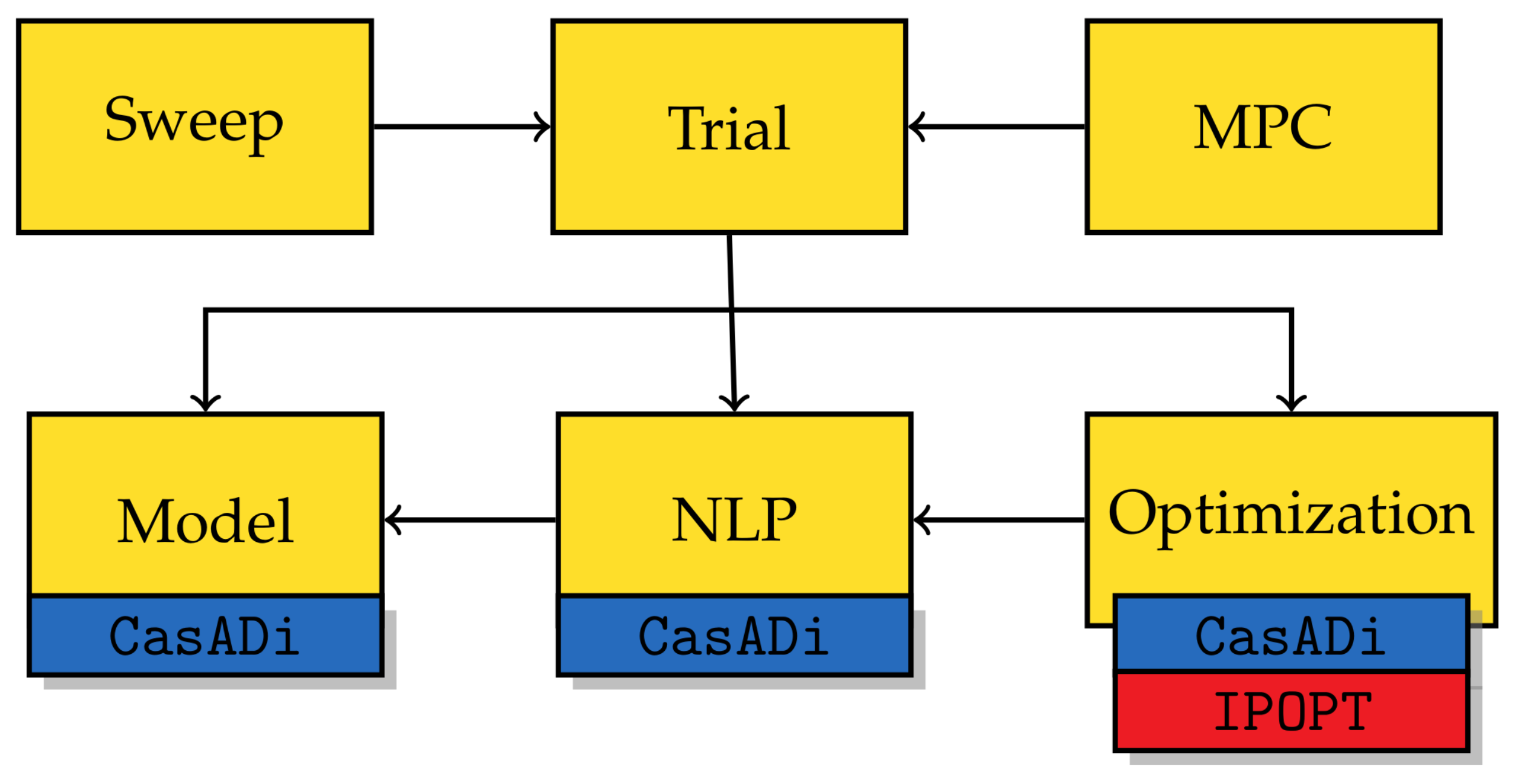The toolbox is written in Python 3 and relies heavily on the following software packages: CasADi, an open-source symbolic framework for algorithmic differentiation and nonlinear optimization [35]; the interior-point NLP solver IPOPT [36]; and (optionally) the linear solver MA57 [51]. The six main classes and the basic structure of the package are shown in Figure 2, including the dependencies on the external packages.

Starting at the lowest level, the Model-class takes the user-provided modeling options and assembles the according state, control, and algebraic variable vectors. Then, the dynamics (1), relevant constraints, and intermediate model outputs are constructed as CasADi Function objects.

Table 1. Main AWE system modeling options and possible variants implemented in awebox.

Options	Variants
Topology	single-aircraft, i.e., $(1,1)$
	multi-aircraft, e.g., $(1,2)$
	stacked multi-aircraft, e.g., $(2,3)$
Power generation	lift-mode
	drag-mode
Aircraft DOF	6 DOF
	3 DOF [10]
Wind profile	uniform
	logarithmic
	power-law
	custom 2D data points
Atmosphere	uniform
	International Standard Atmosphere
	custom data points
Induction	constant/zero
	actuator-disk

gives an overview of the main modeling options implemented in AWEbox. Central here is the use of CasADi to compute the partial derivatives of the system Lagrangian in (16). Finally, the Model class can also be used in standalone mode, e.g., in case the user is interested in obtaining the dynamics for simulation purposes only.

The NLP class the dynamics and constraints receives from a Model instance and constructs the NLP functions ${\mathrm{\Phi }}_{\mathrm{H}}$, ${\mathbf{G}}_{\mathrm{H}}$ and ${\mathbf{H}}_{\mathrm{H}}$ as CasADi Function objects, using the direct collocation approach presented in Section 3.3.

From a practical viewpoint, it is essential for the convergence of the NLP solver that all variables, equations, and cost terms are properly scaled. Therefore, AWEbox implements a heuristics-based scaling procedure based on the system parameters and the user-defined initialization. We refer the reader to the open-source implementation for the scaling factors obtained in the numerical experiments in this study.

The NLP functions are then passed on to the Optimization class, where their first- and second-order derivatives are constructed using CasADi, which also provides the interface to IPOPT. The Optimization class then constructs the initial guess from Section 3.5 and implements both Algorithms 1 and 2 to prepare the homotopy-based initial guess for solving Problem (53). It is also possible to warm-start of the solver with a user-provided initial guess. Finally, Problem (53) is solved up to high accuracy. The default linear solver for computing the Newton step within IPOPT is MUMPS, but in general, higher performance in terms of speed and reliability is reached using the solver MA57, which has to be installed separately.

On a higher level, the central class with which the user interacts is the Trial class, which knits together the functionality of the lower-level classes. To start with, the user can specify modeling options, physical parameters, discretization options, initialization parameters, etc., as in the (non-exhaustive) example given in Listing 1.

Listing 1. Example of AWEbox options that can be specified by the user.

1 opts = {}  2 opts [‘model.topology’] = {1:0}  # parent map P(n)  3 opts [‘model.kite_dof’] = 6  4 opts [‘model.system_type’] = ‘lift_mode’  5 opts [‘model.wind.model’] = ‘uniform’  6 opts [‘model.wind.u_ref’] = 10. # [m/s]  7 opts [‘nlp.N’] = 100  8 opts [‘solver.linear_solver’] = ‘ma57’  9 opts [‘solver.initialization.l_t’] = 400. # [m] 10 opts [‘solver.homotopy.phi.0’] = ‘penalty’ 11 opts [‘solver.homotopy.phi.1’] = ‘penalty’

Based on the specified options, the user can create a Trial object, and build the system dynamics, constraints, and NLP functions, including derivatives, as shown in Listing 2. In this example, the power optimization is then solved using the penalty-based homotopy. The Trial class then performs some quality checks on the numerical accuracy of the solution, e.g., by checking consistency condition satisfaction. The class also contains some basic plotting functionality for visualizing the optimal solution.

Listing 2. Set-up and numerical solution of a periodic OCP via the AWEbox interface.

12 from awebox import Trial 13 trial = Trial(opts) 14 trial.build() 15 trial.solve() 16 trial.plot([‘states’, ‘controls’])

The high-level class Sweep, which builds on the Trial class, can be useful for parametric sweeps, as illustrated by Listing 3. This class builds the parametric NLP functions and their derivatives only once, and implements Algorithm 3 for warm-starting the neighboring NLP problems.

Listing 3. Parametric sweep set-up and numerical solution via the AWEbox interface.

17 from awebox import Sweep 18 sweep_opts = [(‘model.wind.u_ref’, [4,6,8,10,12,14,16])] 19 sweep = Sweep(opts, sweep_opts) 20 sweep.build() 21 sweep.run()

The MPC class uses the Trial class and the lower level classes to construct the tracking MPC problem as defined in [58]. The class takes as an input the optimal solution of Problem (39) to construct a periodic reference on the MPC time grid. It also takes care of correct initialization, an initial guess, and periodic reference shifting. The MPC problem can then be recursively solved using IPOPT with the warm-starting strategy from [57]. The main goal of this class is not to provide highly efficient numerical solvers aimed at embedded optimization, such as those implemented in the software packages acados [59] or PolyMPC [60]. Rather, this class provides a reliable controller that conveniently allows for offline closed-loop simulations. Listing 4 provides an example of how such a controller can be constructed and evaluated based on (solved) Trial-object.

Listing 4. MPC controller set-up and evaluation via the AWEbox interface.

22 from awebox import Pmpc 23 mpc_opts = {} 24 mpc_opts [‘N’] = 20 25 mpc_opts [‘terminal_point_constr’] = True 26 Ts = 0.1 27 mpc = Pmpc(mpc_opts, Ts, trial) 28 u0 = mpc.step(x0)

Although the focus here is reliability and not computational efficiency, the user can also code-generate and compile the MPC solver functions using CasADi for use in an external codebase or for embedded application.

5. Numerical Results

This section discusses two numerical case studies that highlight the contributions of the AWEbox software package. In the first case study, we discuss and compare the computational performance and robustness of the homotopy algorithms CIPH and PIPH, while solving a single-aircraft lift-mode reference problem. In the second case study, we compute a power curve for a dual-aircraft lift-mode system and compare the performance of the algorithms PIPH and SIPH.

In this paper, we focus mainly on algorithmic developments and performance. However, for validation purposes, we also provide an example in the toolbox repository which re-implements the case study performed in [15] with a very good agreement of results. Small remaining discrepancies can be explained by tuning differences since the exact regularization weights and scaling factors used in this case study are not available. For brevity, we do not discuss these results further in this text.

5.1. Single-Aircraft Case Study

The first reference problem aims at finding an optimal power cycle for a lift-mode single-aircraft system, with $\mathcal{K}=\left\{1\right\}$, $\mathcal{L}=\left\{1\right\}$, and $P\left(1\right)=0$. The aircraft parameters are taken from the Ampyx AP2 reference model presented in [22]. We adopt the same wind profile and atmosphere model as presented in [15]. We assume a “reinforced” version of the AP2 airframe since the real-world airframe load limits lead to an overly pessimistic average power output estimate. Therefore, compared to the OCP in [15], the airspeed limits and tether force limits are omitted and replaced only by a tether stress constraint, while the tether diameter $d_{\mathrm{t}}$ is no longer fixed and is treated as an optimization variable. Table A1 in Appendix A summarizes the model parameter values of this reference problem, while

Table 2. System variable bounds and path constraints.

Description	Variable	Min	Max	Units
Side-slip angle	$\beta$	−20.0	20.0	deg
Angle-of-attack	$\alpha$	−6.0	9.0	deg
Tether stress	$\sigma$	0.0	3.6	GPa
Rotation angle	${\gamma }_{\mathrm{r}}$	−40.0	40.0	deg
Tether length	$l_{\mathrm{t}}$	10.0	700.0	m
Tether speed	${\dot{l}}_{\mathrm{t}}$	−15.0	20.0	ms${}^{-1}$
Tether acceleration	${\ddot{l}}_{\mathrm{t}}$	−2.4	2.4	ms${}^{-2}$
Flight altitude	$q_{\mathrm{z}}$	100.0	-	m
Time period	T	20.0	70.0	s
Angular velocity	$\omega$	−50.0	50.0	deg s${}^{-1}$
Aileron deflection	${\delta }_{\mathrm{a}}$	−20.0	20.0	deg
Rudder deflection	${\delta }_{\mathrm{r}}$	−30.0	30.0	deg
Elevator deflection	${\delta }_{\mathrm{e}}$	−30.0	30.0	deg
Deflection rates	$\dot{\delta }$	−2.0	2.0	rad $s^{-1}$

lists all variable bounds and path constraints.

We construct the NLPs (68) and (69) using $N=100$ intervals with Radau collocation polynomials of the order $M=4$, and the controls are discretized using a piecewise constant parameterization. The resulting NLPs have 15,334 variables, 14,323 equality constraints, and 600 inequality constraints. We solve the problem on an Intel Core i7 2.5 GHz, 16GB RAM.

The homotopy meta-parameters are experimentally tuned to minimize the associated CPU time. The intermediate homotopy barrier parameter is chosen as ${\tau }_{\mathrm{i}}={10}^{-2}$. For CIPH, the number of parameter update steps per stage are ${\gamma }_1=10$ and ${\gamma }_2=1$. For PIPH, the homotopy parameter penalties are $S_1={10}^2$ and $S_2=1$.

In the following, we wish to investigate the performance and robustness of CIPH and PIPH, compared to the case where the user-provided circular initial guess is applied without refinement (“no homotopy” - NH). For this purpose, the reference problem described above is solved for each method for a set of 100 uniformly sampled initialization parameters ${\mathbf{\pi }}^0$ from the set defined by ${\mathbf{\pi }}_{\mathrm{lb}}^0\le {\mathbf{\pi }}^0\le {\mathbf{\pi }}_{\mathrm{ub}}^0$.

In the NH-case, performance heavily depends on the a priori knowledge of the user. To account for this fact, we introduce two different users. “User A” is an AWE developer with little a priori knowledge of the location of the optimal solution. Therefore, this user has samples from a wide initialization parameter set. “User B,” on the other hand, is a control engineer who is familiar with the system and its optimal behavior for the given conditions. Therefore, User B samples from a parameter set that is defined by a range that is a factor 3 smaller than that of User A, centered around the average parameters as evaluated at the solution of interest.

Table 3. Initialization parameter bounds used for uniform sampling by users A and B.

Description	Variable	Min (A)	Max (A)	Min (B)	Max (B)	Units
Flight speed	${\dot{q}}^0$	20.0	60.0	30.6	44.0	ms${}^{-1}$
Tether length	$l_{\mathrm{t}}^0$	300.0	600.0	300.0	391.8	m
Elevation angle	${\theta }_{\mathrm{e}}^0$	30.0	50.0	26.3	32.9	deg
Cone angle	${\theta }_{\mathrm{c}}^0$	20.0	30.0	14.9	21.5	deg
Phase angle	${\phi }^0$	0.0	360.0	0.0	93.9	deg
Tether diameter	$d_{\mathrm{t}}^0$	1.0	5.0	1.6	2.9	mm

summarizes the sampling range for all initialization parameters, for both User A and B. The initial number of loops is chosen to be $N_{\mathrm{l}}^0=1$.

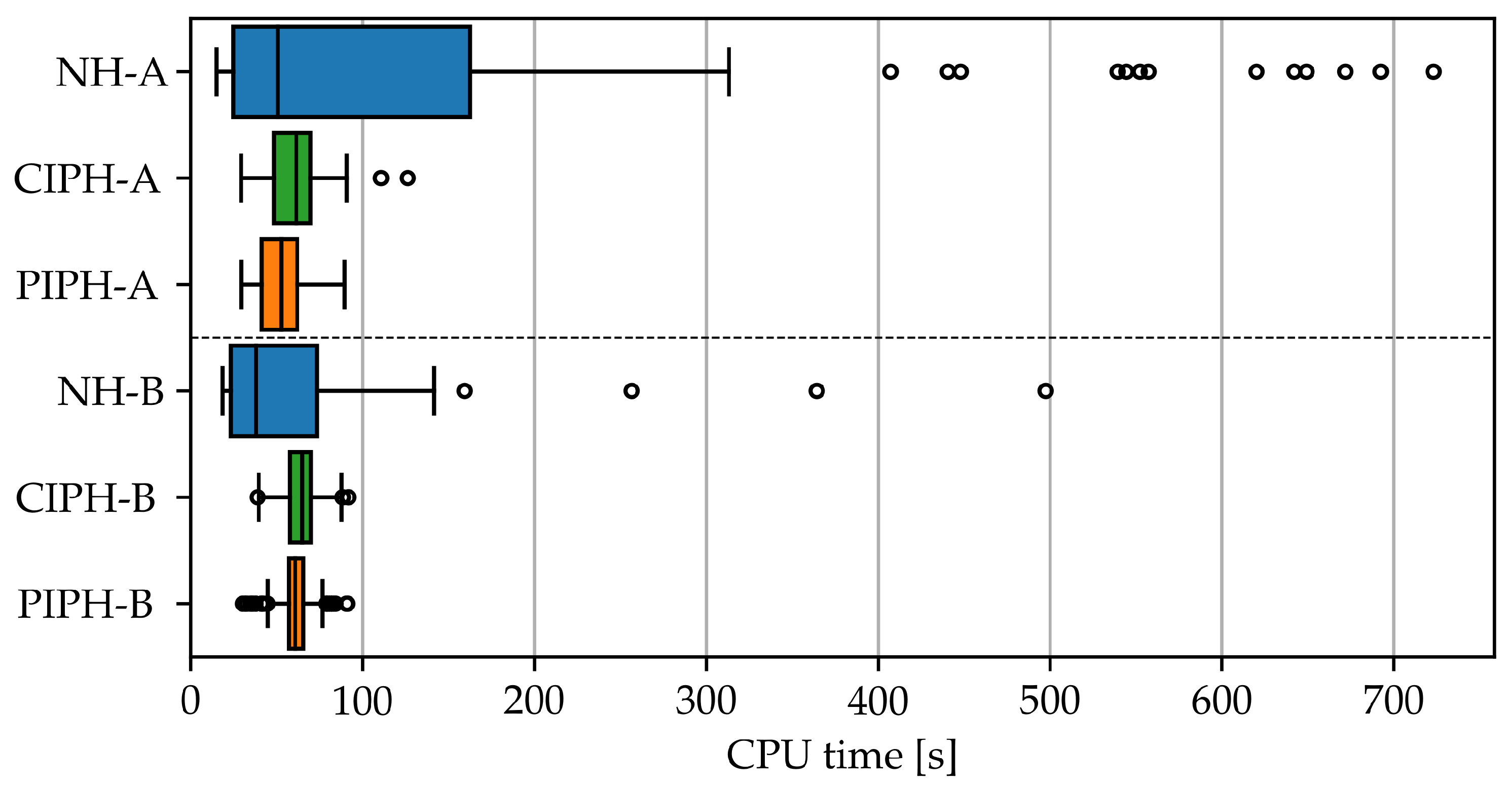
Figure 3 shows the CPU timing results resulting from the initialization sampling by User A and User B. For User A, NH leads to highly variable CPU timings, ranging from a peak timing of up to 12 min down to a minimum of 15 s. In two cases, NH does not converge as it exceeds the maximum number of iterations of the NLP solver. The minimum NH-timing is 50% lower than the best timings of the homotopy methods. Hence, it is possible for User A to “get lucky" and converge to a solution very fast without initialization refinement. However, the peak NH timing is 8 times higher than the worst PIPH timing and almost six times higher than the worst CIPH timing. The average NH timing is a factor of 1.7 times higher than in the PIPH case and a factor of 1.3 higher than in the CIPH case. Therefore, User A benefits significantly from CIPH/PIPH in terms of expected computational performance and, in particular, in terms of timing consistency. PIPH is, on average, 13% faster than CIPH, while the peak timing is 30% lower.

For User B, with much better a priori knowledge, the computation times of NH significantly improve compared to user A: average timings are reduced by a factor of 2.4, to a value slightly lower compared to CIPH/PIPH for User B. The peak NH timing is reduced by a factor of 1.5, which is still a factor 5.5 larger than compared to CIPH/PIPH. Thus, while User B has a slightly better-expected performance in the NH case, he or she can still profit from the improved timing consistency provided by CIPH/PIPH. The difference in timings for the CIPH and PIPH methods is almost negligible. The average timings of these methods do not change much compared to the timings obtained for User A. This highlights the property that by pre-structuring the optimization path, the homotopy methods are not able to exploit a priori user knowledge to achieve better average performance.

Overall the PIPH/CIPH CPU timings range between 30 and 100 s. This is comparable to the CPU timing range reported in [26] for similar model complexity and identical collocation grid (but excluding homotopy timings).

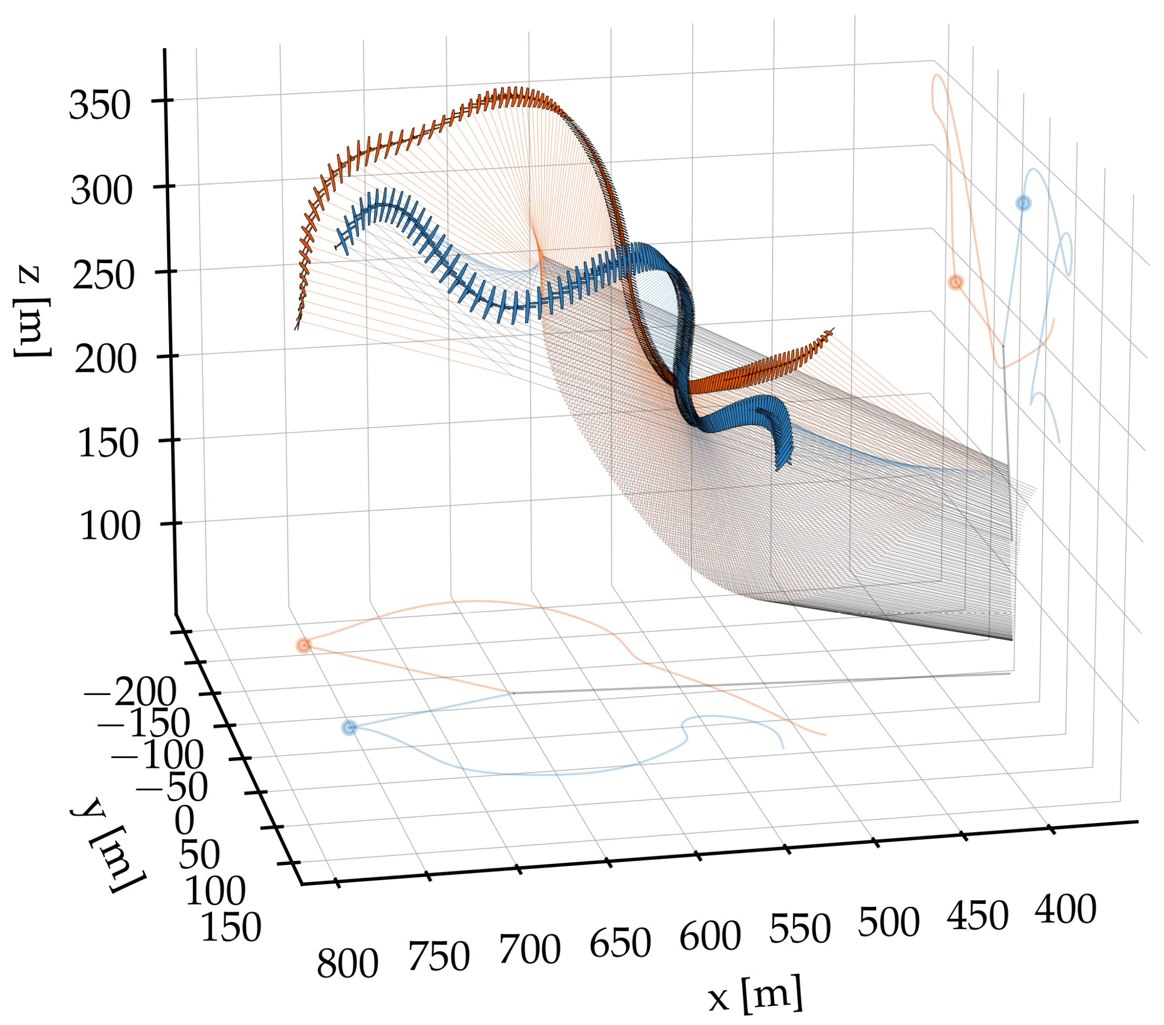
The NLP (53) has multiple local solutions, and the choice of optimization algorithm influences the frequency with which certain solutions are found by the optimizer. In the experiments for User A, a total of nine different local solutions were found. Figure 4 shows the dominant, circular, optimal solution, while Figure 5 shows as an example the third most frequent optimal solution, which is characterized by the well-known lemniscate flight pattern.

Table 4. Frequency of occurrence in a set of 100 trials, optimal time period $T^{*}$, average power output ${\overline{P}}^{*}$, and maximum consistency violation of locally optimal solutions (Nrs. 1 - 9) found by User A.

Nr.	NH	PIPH	CIPH	${\mathit{T}}^{*}$ [s]	${\overline{\mathit{P}}}^{*}$ [kW]	${\parallel \mathit{C}\left({\mathit{x}}^{*}(·)\right)\parallel }_{\mathit{\infty }}$
1	71%	100%	98%	20.2	8.8	8$·{10}^{-4}$
2	15%	-	-	24.0	8.7	9$·{10}^{-4}$
3	7%	-	-	27.9	9.3	1$·{10}^{-3}$
4	1%	-	1 %	32.5	9.0	3$·{10}^{-3}$
5	1%	-	-	41.5	10.7	7$·{10}^{-3}$
6	1%	-	-	41.2	10.6	2$·{10}^{-2}$
7	1%	-	-	47.8	10.0	4$·{10}^{-2}$
8	1%	-	-	37.4	10.3	6$·{10}^{-3}$
9	0%	-	1%	40.4	10.5	1$·{10}^{-2}$
Fail	2%	-	-	-	-	-

summarizes, for each method, the frequency of local solutions.

The homotopy methods almost always converge to the main solution of interest: out of 100 trials, 100 for PIPH, and 98 for CPIH. In the NH case, on the other hand, this is only the case for 71 trials, while failing to converge in two cases. Hence, the homotopy methods not only improve performance and reliability for User A, but they are also more stable in terms of optimization outcome. For User B, all methods always converge to the main solution.

When comparing the different local solutions, we notice that average power output increases up to 22% with respect to the main solution for solutions with longer optimal time periods $T^{*}$. The solutions with a longer time period typically consist of more than one loop, which leads to a better ratio of reel-out vs. reel-in time, and, thus, a higher “pumping efficiency.” This is in line with the results reported in [26].

Note that for increasing time period $T^{*}$, consistency condition satisfaction decreases. This is because the consistency condition trajectory is the periodic solution to the stable uncontrolled dynamics of the invariants. Hence, as simulation accuracy decreases, consistency conditions are moving away from the theoretically optimal solution of a constant zero value. For this reason, AWEbox automatically computes the consistency conditions for each solution and gives out a user warning once a threshold is reached. The user can then increase the number of collocation intervals and the integration order, or lower the upper bound on T if applicable.

5.2. Dual-Aircraft Power Curve

In the second case study, we compute the power curve for a dual-aircraft lift-mode system, i.e., $\mathcal{K}=\{2,3\}$, $\mathcal{L}=\left\{1\right\}$, $P\left(1\right)=0$, $P\left(2\right)=1$, and $P\left(3\right)=1$. We retain the model parameters and constraints and discretization of the single-aircraft case study while adding the anti-collision constraint (44).

To give more structure to the problem, we propose the following modification to the OCP. We divide the time horizon into two separate intervals with associated time variables $T_1$ and $T_2$, and we define the total time period as $T:=T_1+T_2$. We then impose that the first interval is a single reel-out phase, and the second one a single reel-in phase:

$$\begin{array}{cc}\hfill {\dot{l}}_{\mathrm{t}}& \ge 0,\forall t\in \left[0,T_1\right]\hfill \end{array}$$

(73)

$$\begin{array}{cc}\hfill {\dot{l}}_{\mathrm{t}}& \le 0,\forall t\in \left(T_1,T\right].\hfill \end{array}$$

(74)

In the discrete time grid, 70 time intervals are allotted to the reel-out phase, and 30 intervals to the reel-in phase. The resulting NLP has 33,464 variables, 31,550 equality constraints, and 1402 inequality constraints.

The intermediate barrier parameter is tuned manually to be ${\tau }_{\mathrm{i}}={10}^{-4}$ for both PIPH and SIPH. The PIPH tuning is the same as in the single-aircraft case. SIPH performs a homotopy with ${\gamma }_{\mathrm{p}}=10$ steps for every new parameter value. Additionally, the maximum number of NLP solver iterations is limited to 100 for both methods.

We search for solutions with three loops, i.e., $N_{\mathrm{l}}^0=3$. The reason for this is that the resulting trajectories fit well inside the time period bounds defined in Table 2, for all considered wind speeds. The remaining initialization parameters are set to ${\dot{q}}^0=50\frac{\mathrm{m}}{\mathrm{s}}$, ${\theta }_{\mathrm{e}}^0={25}^{\circ }$, ${\theta }_{\mathrm{c}}={20}^{\circ }$, ${\varphi }^0=0^{\circ }$, $l_{\mathrm{t}}^0=640\mathrm{m}$, $l_{\mathrm{s}}^0=100\mathrm{m}$, $d_{\mathrm{t}}^0=4\mathrm{mm}$, and $d_{\mathrm{s}}^0=\frac{1}{\sqrt{2}}{d}_{\mathrm{t}}^0$. The secondary tether diameter is initialized under the assumption that the secondary tether force equals the main tether force divided by two.

The power curve for the proposed dual-aircraft system is obtained in the following manner. First, the optimal trajectory and design are computed with PIPH for a reference wind speed of $u_{\mathrm{ref}}=10\frac{\mathrm{m}}{\mathrm{s}}$. The resulting optimal design is given by $l_{\mathrm{s}}^{*}=142.9\mathrm{m}$, $d_{\mathrm{t}}^{*}=4.3\mathrm{mm}$ and $d_{\mathrm{s}}^{*}=3.2\mathrm{mm}$. The average power output is ${\overline{P}}^{*}=42.0\mathrm{kW}$. Note that this is more than a factor of four higher than the single-aircraft solutions in the first case study, while the number of aircraft has only doubled. The power per wing surface area is thus more than doubled as a result of the reduced main tether drag and higher flight altitude. This is in line with the results reported in [10,12].

The optimal design parameters are then fixed, and the NLP is re-solved for $u_{\mathrm{ref}}$ ranging from 0 $\frac{\mathrm{m}}{\mathrm{s}}$ to 20 $\frac{\mathrm{m}}{\mathrm{s}}$. This is done once with PIPH, every time starting from the identical user-defined initial guess. Then, it is done once using SIPH in two separate sweeps: once downwards and once upwards starting from the solution for $u_{\mathrm{ref}}=10\frac{\mathrm{m}}{\mathrm{s}}$.

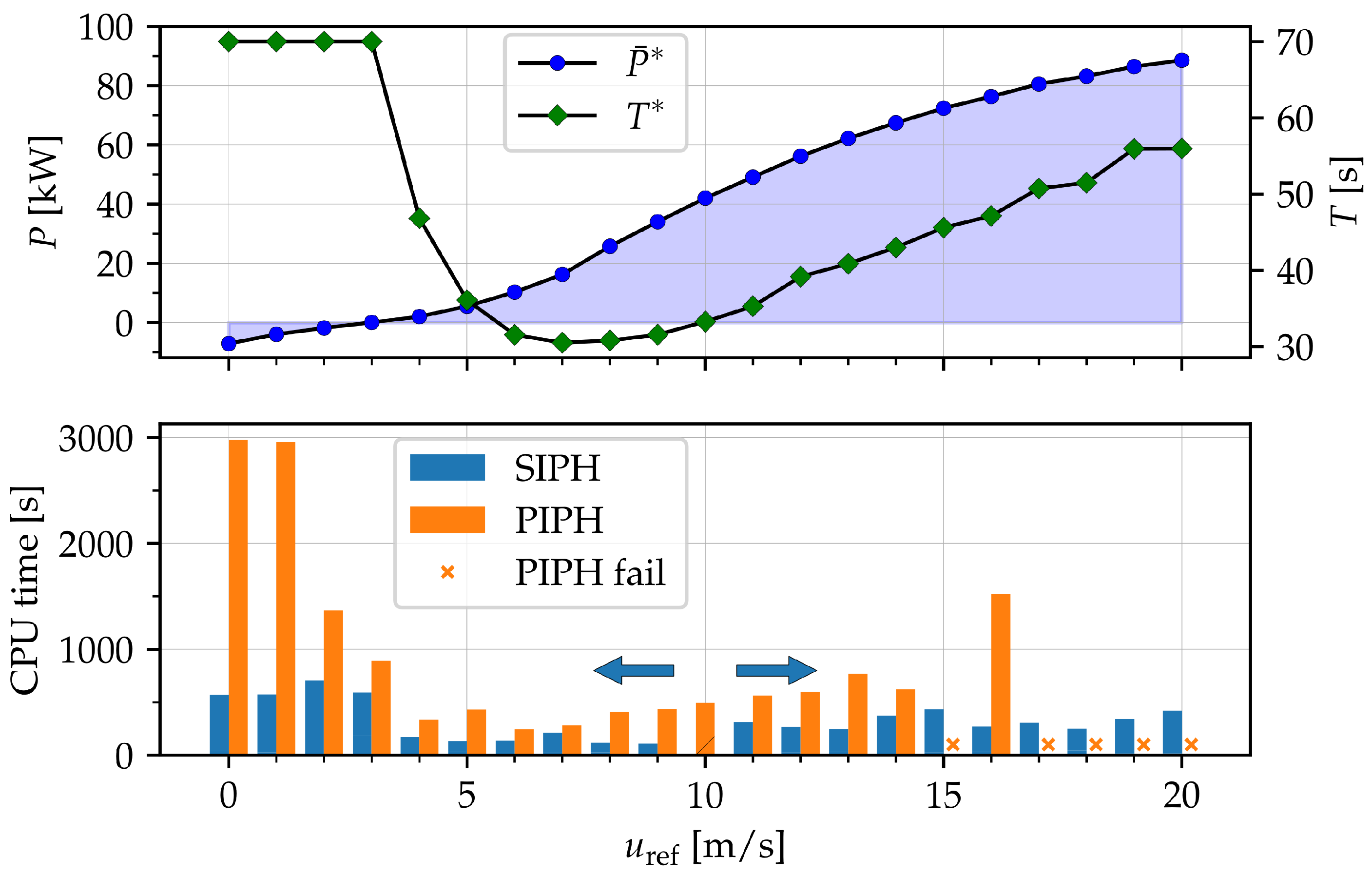
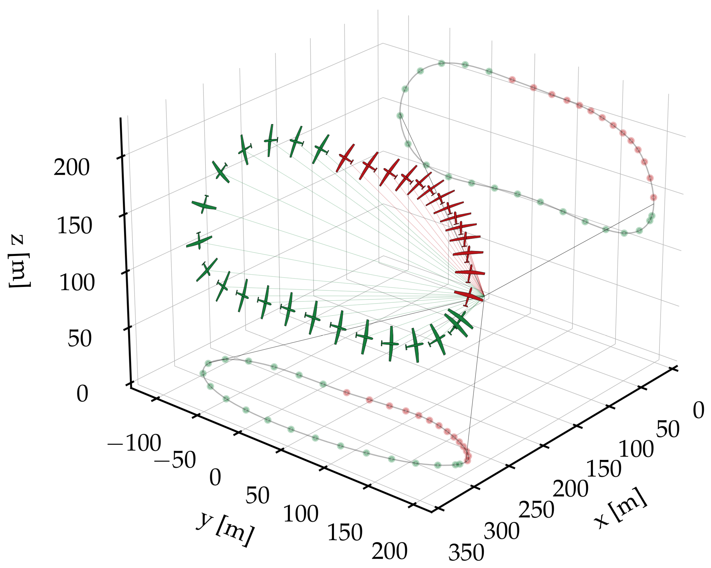
Figure 6 shows the power curve obtained with SIPH, and, additionally, for each wind speed, the optimal time period. Similar to the power curve computed in [37], we identify three operational regions. In the first region of zero wind speed up to the cut-in wind speed $u_{\mathrm{ref}}=3\frac{\mathrm{m}}{\mathrm{s}}$, power is consumed to keep the system airborne. The upper bound on T is active here, as the aircraft glide downwards about an almost vertical rotation axis during the reel-out phase. In the reel-in phase, potential energy is injected back into the system as the aircraft fly slow upward trajectories. In the second operating region, power grows cubically until the design wind speed is reached. In the third region, power output still grows with the wind speed, but cubic growth is curtailed in order to satisfy the tether stress constraints. The main strategy to limit power output here is to increase the tether reel-out speed so as the decrease the available wind. The optimal time period increases with respect to the design wind speed, as the reel-out speed increases, while the reel-in speed is constrained and cannot grow proportionally. 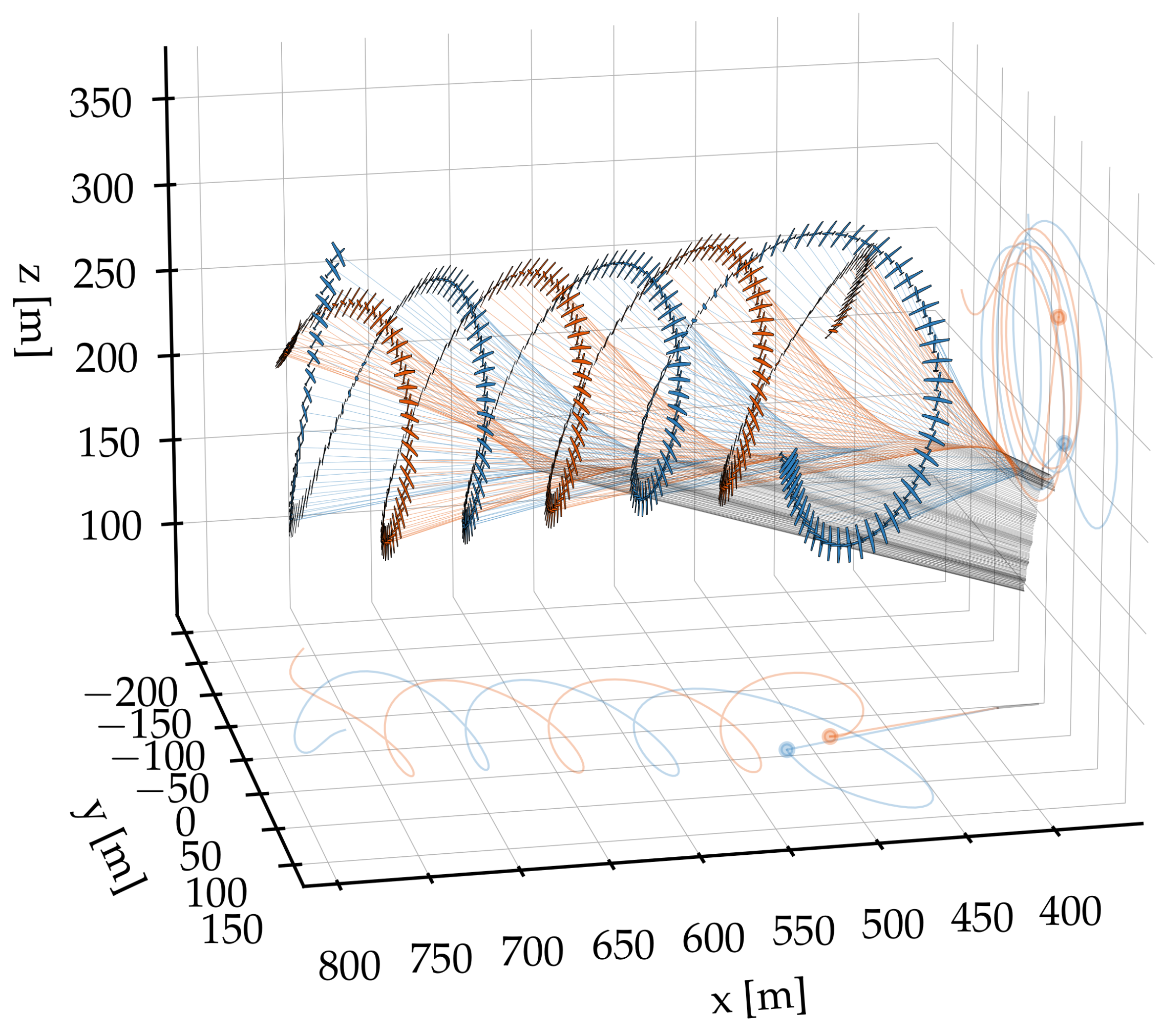Figure 7 and Figure 8 illustrate the reel-out and reel-in trajectories for $u_{\mathrm{ref}}=18\frac{\mathrm{m}}{\mathrm{s}}$.

Figure 6 also shows for each wind speed the associated CPU time for PIPH and SIPH. The computation times include both the CPU time for the homotopy procedures and the CPU time to solve the final problem ${\mathcal{P}}_{\mathrm{f}}$. PIPH does not converge for the wind speeds of 15 $\frac{\mathrm{m}}{\mathrm{s}}$ and 17 to 20 $\frac{\mathrm{m}}{\mathrm{s}}$. Note that convergence might be recovered for smaller update steps of the homotopy parameter $\overline{\mathbf{\varphi }}$. However, this falls outside the scope of this study.

SIPH outperforms PIPH at every single wind speed (where PIPH converges), but particularly at low wind speeds, when the optimal solution diverges significantly from the user-defined initial guess. Up until the wind speed of 15 $\frac{\mathrm{m}}{\mathrm{s}}$, the average CPU time is 5 min and 23 s for SIPH and 15 min and 20 s for PIPH.

6. Discussion

In this work, we presented AWEbox, an open-source Python toolbox for the modeling and optimal control of single- and multi-aircraft AWE systems. We discussed the general multi-aircraft modeling structure, optimization ingredients, and implementation details needed to efficiently compute power-optimal orbits for a wide range of system architectures and modeling options. In particular, we proposed and implemented two interior-point-based homotopy method variants, in order to increase the performance and reliability of the optimization algorithms. These methods produce a feasible initial guess for the underlying NLP solver, based on an analytic initial guess shaped by the software user. In a numerical experiment, a reference single-aircraft problem was solved for a large set of different initial guesses.

The penalty-based homotopy method reduced the average and peak CPU timing with a factor of 1.7 and 8, respectively, compared to the case when no homotopy method was applied by a user with little a priori knowledge. With good a priori knowledge available, the homotopy methods did not improve performance, but still, the peak CPU timing was reduced by a factor of 5.5. Overall, computation times were in the range of 30–100 s, which is competitive with those reported in the literature. Additionally, the penalty-based homotopy method consistently led to the same local solution, whereas the no-homotopy case resulted in different local solutions in 29 out of 100 cases.

In a second case study, we computed a power curve of a dual-aircraft AWE system and compared the performance of the penalty-based homotopy method of the previous case study with that of a third homotopy method tailored for parametric sweeps with interior-point NLP solvers. The penalty-based method was not able to converge to a solution for all wind speeds, while the sweep method succeeded in doing so while outperforming the penalty-based method, on average, by a factor of three in terms of CPU timings. The average CPU timing per NLP solution was about 5 min.

Future work might entail model accuracy improvements, in particular concerning tether and induction modeling The tether model can be readily improved to include sagging by discretizing the tethers into finite elements, linked by algebraic constraints as proposed in [10]. On the problem formulation side, it can be investigated in which cases global-support direct collocation using Fourier approximations can improve efficiency in terms of CPU time and memory usage. Efficient problem formulations and implementations that include stability and robustness considerations would be a useful contribution, in particular for multi-aircraft systems. Finally, efficient algorithms that enable simultaneous trajectory and design optimization with expensive models (e.g., aero-elastic models) could lead to faster and more accurate system design loops.