Application of Planar Laser-Induced Fluorescence for Interfacial Transfer Phenomena

Abstract

The present review describes the current achievements in the applications of a planar laser-induced fluorescence (PLIF) method for the diagnostics of liquid films, bubbles, individual droplets, and sprays. Such flows are related with strongly curved interphases, which often results in additional high errors during the PLIF data quantification because of laser light reflection, refraction, and absorption. The present review demonstrates that a two-color PLIF approach and a PLIF modification for regularly structured illumination resolves the reflection- and refraction-caused errors. The latter modification ensures proper phase separation in the measurement cross-section and visualization of the interface dynamics. The former approach provides the accurate evaluation of the local temperature and concentration both in liquid and gaseous phases even in the case of strong variations of the laser sheet intensity. With intensified cameras, the PLIF method is used for multi-parameter diagnostics of the two-phase combustion of sprays in combustion chambers with optical access. It visualizes and quantifies the liquid fuel evaporation and mixing, to measure temperature in the gas and liquid phases and to reveal the regions of pollutant formation. The PLIF technique can also be easily combined with a particle image (or tracking) velocimetry method, to evaluate local heat and mass transfer.

1. Introduction

The Planar Laser-Induced Fluorescence (PLIF) technique has become a powerful tool for the quantitative imaging of heat and mass transfer and chemical reactions in different applications of single-phase and multi-phase flows, ranging from micro- and nanoscale fluidic devices and biological samples to large-scale industrial applications. The current development of the PLIF technique for micro- and nanoscale problems pursues the super-resolution imaging of molecular transport, chemical reactions, properties of cells and their interactions, and single-molecule spectroscopy [1,2,3,4,5,6,7]. The operation of many industrial rigs and chemical reactors is related with interfacial transfer phenomena in two-phase flows, such as liquid films and bubbles, droplets, and sprays. These flows are associated with intensive interphase heat and mass transfer during boiling and cavitation, evaporation and adsorption, freezing and solidification, and often with chemical reactions, such as spray combustion. The application of PLIF methods allows for the study of these complex problems in details (e.g., see [8,9,10,11,12,13,14]) to improve the efficiency of heat exchangers, powder sprinklers, chemical reactors, combustors, and other devices. However, the extraction of quantitative information from the raw PLIF images relies on a number of data processing routines, including the spatial calibration of images, absorption/attenuation correction, linearity verification, compensation of the spatial non-uniformity of detector sensitivity, and illumination (see [15,16,17,18,19], among others).

Liquid films are conventionally defined thin layers of liquid between a solid surface and gaseous environment. The case when there is a contact line between the solid surface, liquid layer, and gaseous environment is usually referred to as a rivulet flow. Liquid films often form as a liquid layer between two regions, filled with gas, such as the walls of a soap bubble or a planar/annular liquid sheet in air-blast or simplex atomizers. An obvious example of the film flows is a gravity-driven thin liquid layer over a vertical or inclined plate, which is commonly used in chemical reactors, food industry, painting technology, and decorative installations. The lubrication oil in complex machinery usually forms a film over the mechanical parts of equipment. Liquid film flowing over corrugated surfaces is common in distillation columns, refrigeration, evaporators, and desalinators. Thin liquid films are formed around Taylor bubbles in slug and churn regimes of gas-liquid and liquid-liquid flows.

The flow of the gas-liquid mixture with high superficial velocity of the gas phase would eventually transform into an annular gas-liquid flow, where liquid film flows along the duct walls being sheared by the high-velocity gas stream in the duct center. The multiphase flow regimes from slug to annular are common in the production and transportation of hydrocarbons, nuclear reactors, propulsion engines, solar energy plants, cooling systems, mucus transport in human airways, etc. Liquid films are formed when a spray or jet of liquid impacts a solid surface, which is related to diesel engines and spray cooling systems. There are numerous methods of film thickness measurements based on different physical principles (see, e.g., [20,21,22]). These include conductance/capacitance techniques, shadow imaging, absorption of radiation (including visible and near-infrared light, gamma-rays, and X-rays), methods based on light reflection (Laser-Focus Displacement, Chromatic Confocal Imaging, and total internal reflection), refraction of light (e.g., Synthetic Schlieren technique), ultra-sonic reflection technique, etc. Two widely used methods of film thickness measurements employ the phenomenon of Laser-Induced Fluorescence (LIF), i.e., the absorption and re-emission of incident light using a fluorescent dye dissolved in fluid.

Bubbly flows are frequently encountered in nature and have several practical applications. In turbulent flows, the presence of bubbles provides mutual interactions of continuous and dispersed phases and results in the complication of a flow structure in comparison to the single-phase case. Starting from the works by Serizava et al. [23], there is a lot of experiments presented in the literature on studying the suppression or enhancement of turbulence by the bubbly dispersed phase. Depending on the size of bubbles and characteristic scales of turbulence, various effects can be observed [24]. The trajectories of bubbles can be affected by the anisotropic turbulence in liquid (turbulent dispersion), while the motion of the bubbles and their agglomerates have an impact on the turbulence in liquid (turbulence modulation) due to a number of physical mechanisms. In order to study the complex structure and mechanisms of mutual interaction between the phases in bubbly turbulent flows in detail, it is necessary to retrieve spatial distributions of liquid and bubbles velocities, as well as the locations of bubbles.

Apart from pointwise measurement techniques, such as the electro-diffusion method [25] and widely used optical fiber probes, there is a number of non-intrusive optical techniques for the planar diagnostics of two-phase flows. The Shadow photography [26,27] Technique (ST) is used extensively for the measurements of locations and shapes of bubbles when the bubble shadow detection faces no difficulties. The main advantage of ST is that it can be easily combined with Particle Image Velocimetry (PIV) or Particle Tracking Velocimetry (PTV) techniques, when fluorescent tracers are used for the seeding of the carrier liquid phase. Such a combination requires two (or even more) cameras with appropriate optical filters and a diffusive light source (e.g., LED-array with a diffusive screen) with an emission spectrum at distinct wavelengths than that of the laser source and those of fluorescence by the tracers. The combination of ST and PIV-LIF allows for the detailed study of the dynamics of bubbles and their interaction with liquid. One of the main problems faced in ST is the overlapping of bubbles on images when void fraction is high enough. Nevertheless, the ST has been used extensively for bubble detection in narrow column or channel flows for volumetric contents of gas fraction up to 10%.

The characteristics of heat and mass transfer processes in droplets of liquid in gas flow or on a solid wall are needed when predicting the operation parameters of a wide group of setups (for example, surface heat exchangers, counterflow and drip cooling towers, evaporative cooling and spray drying systems, coating technologies, atomization of fuels in combustion chambers, flue gas cleaning, etc.). Starting from the middle of the last century, theoretical and experimental studies on the characteristics of heating and the evaporation of liquid droplets under the conditions of conductive, convective, and mixed heat transfer have been actively performed [28,29,30,31]. The analysis of reviews [32,33] shows that the problem of determining the rates of heating and evaporation of droplets remains the most relevant today. The numerical values of these parameters can be found primarily by analyzing the dynamics of droplet temperature changes [34,35,36,37]. Until now, the most common approach for the evaluation of droplet temperature was the technology of thermocouple measurements [38,39,40,41,42].

For liquid droplets, as a rule, miniature fast-response thermocouples with a junction diameter of several hundred microns are used [39,40]. Along with the availability and simplicity of this approach [38,39,40,41,42,43], its application in practice has a number of significant drawbacks: radiation losses; the thermocouple junction can significantly affect the temperature inside the droplet; limited temporal and spatial resolution; and pointwise measurements. It is very difficult to measure the temperature inside a moving droplet (especially an aerosol droplet). In recent years, the PLIF method has been widely used to study the processes of liquid droplet heating and evaporation. The results obtained can be conditionally divided into three subgroups: droplets suspended on holders; drops on hard surfaces; and droplets in a free fall or in a flow (including sprays). Further, within the scope of the present work, the achievements of the PLIF applications, as well as the limitations of this method, will be described.

The analysis of sprays, produced by different types of injectors, basically relies on direct and ST visualization with a short-pulse illumination to retrieve the overall spray shape and resolve possible defects of atomization, such as liquid jets, etc. The measurement accuracy, acquisition frequency, and spatial resolution of ST based on X-ray radiography have been improved sufficiently [44,45]. It is used for the spray diagnostics in optically non-transparent configurations. Diffraction-based particle-sizing instruments are commonly used for the quantitative optical characterization of the spraying quality [46]. The pointwise droplet size and velocity measurements are available by using the Phase Doppler Particle Analyzer (PDPA) [47] and Time-shift [48] techniques. These two methods are well-established and robust for the laboratory and industrial diagnostics of sprays (usually without combustion). However, for the detailed analysis of unsteady sprays and sprays with combustion, planar methods are indispensable. The PLIF method in combination with Mie scattering imaging (often also processed using PIV/PTV) are successfully applied for the visualization of droplet dynamics and fuel vapor concentrations [8,9,14]. Besides, an interferometric droplet sizing (referred to as ILIDS and IPI) [49,50] can be used for the sizing of micron-scale droplets by using ordinary optical lenses without special long-distance microscope optics.

In the present review, we limit our scope using basic and well-established approaches and optical configurations of the PLIF method for the imaging of heat and mass transfer in basic two-phase flow configurations with strongly curved interphases: liquid films, bubbles, and droplets (including sprays with combustion). The present review demonstrates that a two-color PLIF approach and a PLIF method for regularly structured illumination have proved to resolve the reflection- and refraction-caused errors and to separate the interphase in the measurement cross-section. A multi-spectral PLIF imaging for different kinds of molecules provides the evaluation of temperature and concentration distributions both in gaseous and liquid phases.

2. Liquid Films

Here, we consider only the cases when a liquid layer is bounded between a solid wall and gas. The main parameter characterizing the liquid films is their thickness, i.e., the shortest distance from the solid wall to the interface. In the majority of practical applications, the interface between the liquid and gas is not fixed and the film thickness varies in time and space. Thus, the measurement technique should provide the value of the local instantaneous film thickness with the characteristic temporal and spatial resolution better than the smallest corresponding scales of the flow. Obviously, the more complex the shape of film surface and its spatiotemporal dynamics, the stronger the requirements for the measurement technique. Ideally, the measurements should be resolved on two spatial coordinates and time; the spatial domain should be large enough to cover the important stages of flow transformation.

Two widely used methods for film thickness measurements employ the fluorescence phenomenon, i.e., the absorption and re-emission of incident light by molecules of a fluorescent dye, dissolved in working liquid. For the effective excitation of a specific fluorescent dye, a monochromatic light source with the wavelength close to the position of the maximum in the dye absorption spectrum is required. The emission spectrum is shifted toward larger wavelengths due to the non-radiative energy losses by the molecules (Stokes’ shift), which allows one to separate the re-emitted light (fluorescence) from the exciting light using a long-pass optical filter. For dyes emitting in the visible spectrum, the fluorescence intensity can be measured with a simple optical camera. The fluorescence intensity depends on the intensity of the laser light, dye photochemical properties, dye concentration, and solvent properties. When applied for the thickness measurements, the LIF technique has a number of limitations and may yield significant over- or underestimations of the real film thickness; thus, the LIF results should be handled with a great care. Only some of these issues were reported in earlier works. In the present chapter, we conduct a systematic analysis of shortcomings and drawbacks along with possible ways to reduce the error.

One of the aforementioned LIF approaches (in recent papers, it is called Brightness-Based LIF or BBLIF) is based on the interrelation between the thickness of a liquid layer and fluorescence intensity emitted by this layer. Each camera pixel collects the fluorescence intensity along a ray passing through the liquid film. The whole length of this ray inside the liquid should be illuminated by the light of a pulsed laser. Usually, the optical orientation of the camera and the laser direction in the BBLIF nearly coincide. The integral value of fluorescence can be recalculated into the film thickness by integrating the Beer–Lambert law. This method allows for evaluating the film thickness over two spatial coordinates (e.g., see the recent examples [51,52,53]).

The planar LIF imaging across the films (i.e., the PLIF method) flows is based on the illumination of the cross-section orthogonal to the wall, whereas the camera is oriented under a large angle to the plane of the laser sheet. In this case, the thickness of the liquid film is measured directly based on the size of the glowing area in the camera image. Thus, in contrast to BBLIF, the PLIF method does not rely on the exact value of fluorescence intensity: the fluorescence serves only as a marker, denoting the presence of dye-doped liquid in a particular spatial area. This circumstance causes PLIF to be a very simple and straightforward way of obtaining film thickness measurements.

Table 1. A summary of experimental works employing PLIF for film thickness measurements. “X”/“Y”—measurement plane is along/across the flow direction; “W”/”I”—camera and laser are directed from the wall/interphase side; “A”—acute angle in unspecified; “C”,”V”, and “T” indicate velocity, concentration, and temperature measurements, respectively.

Ref.	The Object under Study	Laser/Camera	Angle θ	Sheet/Flow	Add. Meas.
[54]	Falling film on a plate	W/W	35	X	V
[55]		I/W	90	X	C
[56]		W/I	55	Y	-
[57]		W/W	35	X	V
[58]		I/I	71	X	T
[59]		W/W	30	X	-
[60]	Gas-sheared film on a plate	W/W	90	X	-
[61]		I/I	A	X	-
[62]		W/W	90	X	-
[63]		I/W	90	X	-
[64]	Gas-liquid annular/slug/falling film flow in a vertical pipe	W/W	90	X	-
[65]		W/W	90	X	-
[66]		W/W	90	X	T
[67]		W/W	90	X	C
[68]		W/W	90, 70	X	B
[69]		W/W	75	X	-
[70]		W/W	90, 70	X	-
[71]		W/W	90	X	-
[72]		W/W	90	X	-
[73]		W/W	40	X	-
[74]		W/W	90	X	-
[75]	Gas-liquid annular/slug flow in a horizontal pipe	W/W	90	X	-
[76]		W/W	45	X, Y	-
[77]		W/I	A	Y	-
[78]		W/W	90	X	V
[79]		W/I	A	Y	-
[80]		W/W	90	X	-
[81]		W/W	45	Y	-
[82]	Stratified gas-sheared flow	I/I	85	X	-
[83]		W/I	62	X	V
[84]		I/I	A	X	-
[85]		I/W	90	X	V
[86]		I/I	30, 50, 90	X	-
[87]		W/W	70	X	V
[88]	Falling film on outer surface of a horizontal pipe	I/I	A	Y	-
[89]		I/I	90	Y	-
[90]		I/I	90	Y	-
[91]		I/I	90	Y	-
[92]	Liquid-liquid flow in a pipe	I/I	A	Y	-
[93]		I/I	90	Y	-
[94]		I/I	90	Y	-
[92]		I/I	90	Y	-
[95]	Spray-generated film on a plate	W/W	90	X	-

provides a summary of PLIF-studies of various liquid film flows. The first column lists the relevant papers; the second column marks the groups of flows under study. Since the film thickness measurements using PLIF are not directly related to the fluorescence properties, neither the used laser type nor the dye characteristics are specified.

The third column describes the layout of the laser and camera, whether they are directed to the investigated section through the duct wall (W) or through the interface (I). Most often, both the laser and the camera are directed to the investigated liquid film through the duct walls (see Figure 1a). The advantage of this approach is that the effect of the agitated interface on the measurements is minimized. However, the rays leading to the camera may undergo refraction both on the inner and outer borders of the wall. This leads to the distortion of the image, especially for circular pipes. A method to compensate such distortions is to use the pipe with the material with a refractive index close to that of the working liquid (e.g., water is matched by the fluorinated ethylene propylene, FEP) and to enclose the pipe in a rectangular optical box. However, the investigation through the wall is impossible in some cases, e.g., when the liquid flows over a non-transparent surface. In this case, both the laser and the camera rays penetrate the film through the interface (see Figure 1b). The laser sheet illuminates a section of the film surface and the film thickness can be estimated based on the position of the illuminated line in the camera image. Sometimes, if only the position of the interface is of interest, the measurements can be obtained without using fluorescence. Thus, opaque liquid [96] or infrared radiation [97] may be used so the camera detects only the radiation reflected from the interface.

The fourth column specifies the angle θ between the laser sheet plane and the camera. The angle between the camera axis and the laser sheet, θ, is most often equal to 90°. However, smaller angles (down to 30°) are employed sometimes in order to avoid undesired optical effects, as will be described below. The letter “A” in Table 1 denotes an unspecified acute angle. The fifth column indicates whether the investigated section was oriented along the flow (X) or across the flow (Y). The former is mainly aimed at studying the flow development and wave propagation and the latter—at studying the three-dimensionality of the flow. The last column denotes whether any additional measurements were carried out using the same laser sheet. Here, letters “V”, “T”, and “C” denote the planar measurements of liquid velocity, temperature, and the concentration of additives (mainly oxygen), respectively. The letter “B” denotes the simultaneous measurements of film thickness using the BBLIF approach.

Despite its apparent simplicity, the PLIF method has certain limitations and may encounter numerous methodological difficulties. The list of shortcomings and distortion sources is provided below.

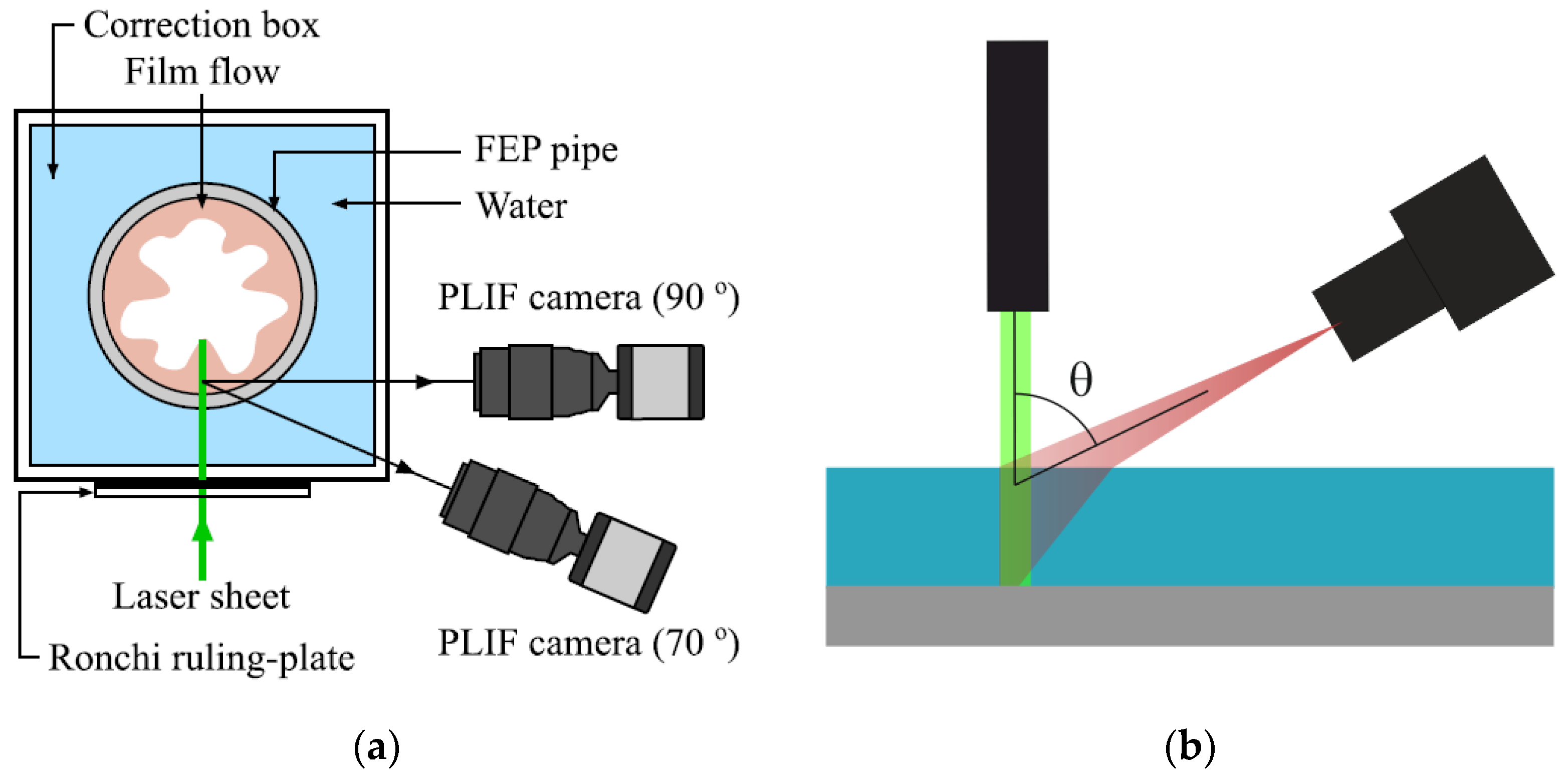
• The PLIF measurements of the film thickness are limited to one section of the film. This causes it to be inappropriate to study flows with essentially three-dimensional waves and other flow structures. A way to overcome this limitation is to employ a scanning device, as in [82,86,98]. In this case, the laser beam hits an inclined mirror before being converted into a laser sheet. The mirror angle is changed by small steps; as a result, the laser sheet is shifted normally to its orientation. This way, the instantaneous film thickness can be obtained in a number of flow sections parallel to each other. Obviously, the full period of mirror rotation and acquisition of the whole set of images must be much smaller than the characteristic time of the flow under study.
• The accuracy of the film thickness measurements is limited by the optical resolution during the imaging. If the angle θ is less than 90°, the resolution—and the accuracy of the measurements—is coarsened as sin⁻¹ θ. When the camera is viewing the illuminated film section through an interface, the actual value of θ will be further reduced due to refraction, according to Snell’s law. Obviously, the thinner the film under study, the better spatial resolution is required.
• As a consequence, there exists a strong limitation on the maximum size of the region of interrogation (RoI). If the RoI size is increased, the spatial resolution and, hence, accuracy of the film thickness measurements decreases. Thus, the long-scale evolution of the thin films cannot be studied with a single camera. Let us consider a film with thickness h studied with a camera with N pixels along the longest dimension of its matrix and the acceptable relative error set to d. Then, the spatial resolution is defined as a = h/d and the maximum length of RoI is defined as L = Na = Nh/d. The intensity-based techniques are free of this limitation, since the accuracy of film thickness measurements in this case is defined by factors independent from the spatial resolution.
• The measurement accuracy is generally worse than that of the intensity-based methods due to the limited spatial resolution. The border of the bright area in the PLIF-images is usually blurred over a certain spatial domain, which is typically larger than the spatial resolution (see examples of fluorescence intensity profiles across the film in Figure 2). Partially, it is related to the Gaussian shape of the laser intensity across the sheet. The presence of the false film image (see below), local transverse slopes of the agitated interface, and reduction in the θ-angle intensify the blurring. There are several approaches to select the point in the blurred area corresponding to the assumed true position of the interface, applied with a different degree of justification and success.

5.

If an interface is present on the optical path from a fluorescing area of the liquid to the camera pixel, the ray will be either totally internally reflected or at least significantly refracted. In any case, the corresponding pixel of the camera remains dark; hence, a false-negative error of film identification occurs and the local film thickness is underestimated. Decreasing the value of θ helps to reduce the probability of such distortion, at the expense of lower resolution as described in (2) and (4) above.

6.

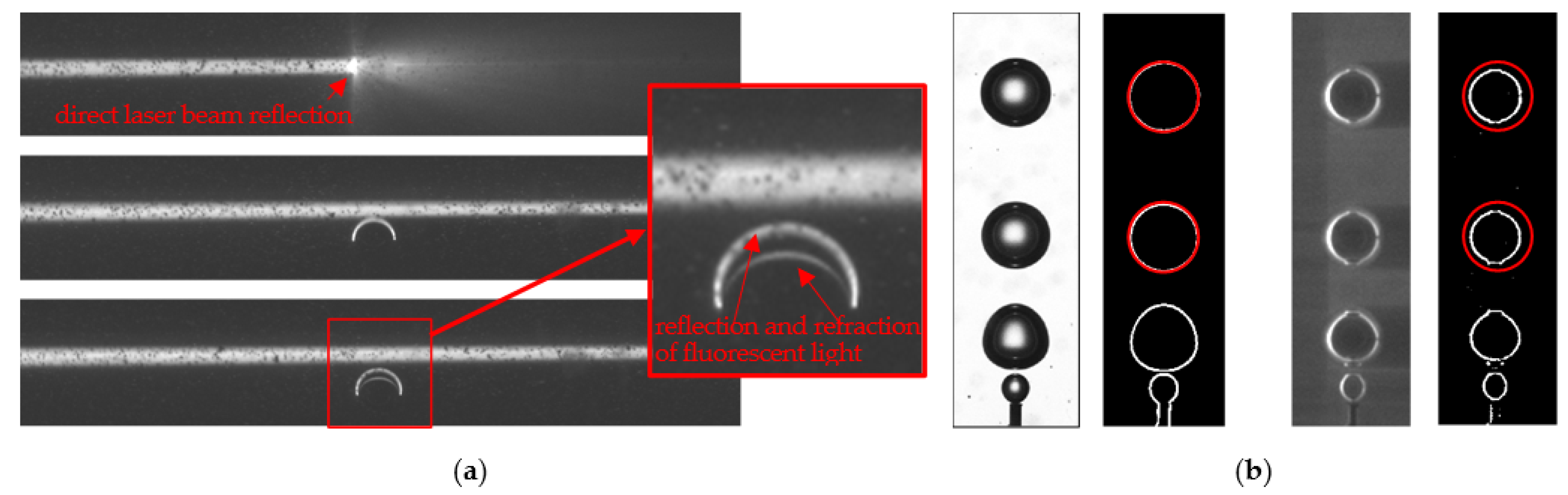
Though the laser light passes only within the sheet, the fluorescence is emitted in all directions. The rays emitted directly into the camera create the true image of the film in the camera matrix. However, the rays emitted in other directions may be reflected by the interface between the laser sheet and the camera into another region of the camera matrix, creating a false film image. For the case of a circular pipe flow and θ = 90°, the calculation of such rays and created true and false film images are shown in Figure 3 [99]. If the angle of incidence of a ray creating the false image is close or larger than the angle of total internal reflection (referred to as the TIR-angle, which is around 48° for water-air interface), the false image will have the same brightness as the true image. The false image is adjacent to the true image and it is nearly impossible to distinguish between them based merely on the local brightness level. For the film with a constant thickness, the false image width is approximately 30% of the true image, see Figure 3b [99]. This phenomenon could be treated as a false-positive error of film identification and overestimation of the film thickness. Sometimes, either a bright or dark line can be seen in the images, marking the position of the true interface [68], see Figure 4a. However, this is not always the case. At lower θ, the false image will increase substantially [68]. Decreasing θ below the TIR-angle may help to darken the false image [68,73], sacrificing the spatial resolution and the sharpness of the image border. For a flat film on a plate, illuminated by a laser sheet normal to the interface and observed under an acute angle θ, the false image will be of the same size as the true film image. Fortunately, if θ is smaller than the TIR-angle, the false image will be much darker, and the true interface could be detected (see Figure 4b). This is why low θ of 30–35° was used in [54,57,59] with the same drawbacks.

An alternative way to separate the true and false image is to use a modified laser sheet. In [68], it was noticed that straight shadows cast by non-uniformities of the pipe are broken at the true interface (see Figure 4a). In [69,70], a structured (periodically blackened) laser sheet was employed to detect the true interface based on the breaking shadows (Figure 5). The main drawback of this approach is an effective coarsening of spatial resolution in the direction of the laser sheet, since the film thickness measurements are actually only obtained in the blackened areas.

It is also important to understand that the apparent (true + false) film image does not physically correspond to the true film image stretched, e.g., 1.3 times. The false image is actually the true image turned upside down and compressed. The true image of the interface remains inside the apparent image. Besides, the dark part of the PLIF-image “above” the film image does not show the gas area above the illuminated film section: it appears due to total internal reflection of the rays leading to the camera outside the pipe. This, in particular, means that the phenomena such as the droplet entrainment or wave overturning cannot be seen using PLIF through a pipe wall. Some more detailed analysis is provided in [100].

7.

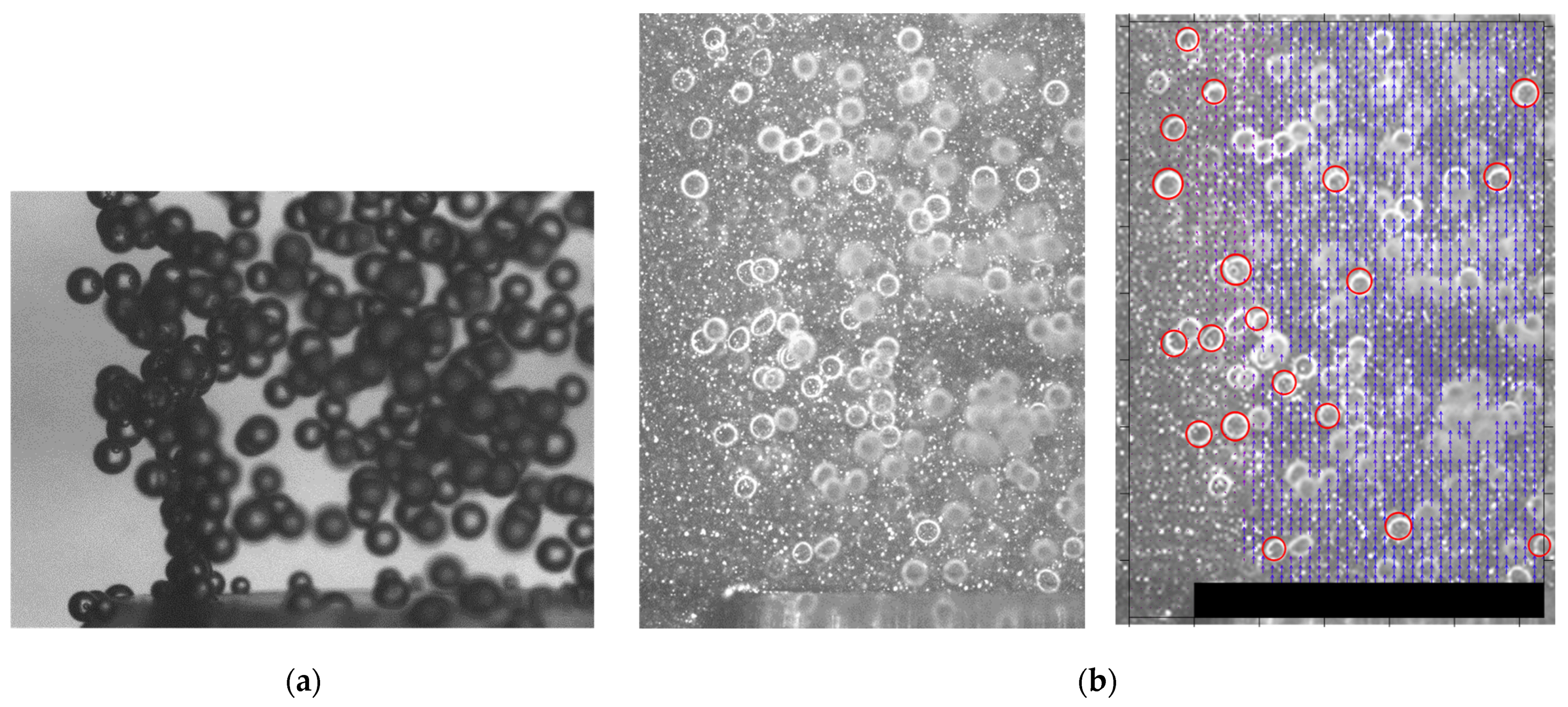
The rays leading to the camera viewing the RoI through the duct wall have a long optical path in liquid. This may be a problem if the liquid film is seeded with bubbles. Numerous bubbles are common in boiling flows [87] and in adiabatic annular flow at high gas speeds [101]. The reduction in liquid surface tension and increase in liquid viscosity increase the number of bubbles [102]. The probability that a ray leading to the camera will be broken by a bubble located between the laser sheet and the camera increases with the length of the optical path in the liquid and the density of the bubbles. In this case, the investigated section of the film will be hidden from view (Figure 6), causing the film thickness measurements to be impossible. For comparison, the intensity-based techniques access the investigated film section directly and only the bubbles located exactly in the investigated section may affect the measurements. The length of the optical path can be decreased by decreasing the θ angle.

It should be also noted that the issues (5–7) are less crucial for liquid-liquid flows, where the refractive indices of both phases are close to each other. The film thickness—no matter how well the measurements are resolved—merely characterizes the first level of complexity of the film flows, namely, the location of the interface. The more detailed measurements may include the characterization of the velocity field in a liquid film, which brings much insight into the flow physics even in purely hydrodynamic studies. In the case of flows with heat transfer, it is necessary to obtain the instantaneous temperature field across the investigated film section. The concentration of chemical additives (e.g., dissolved oxygen) should be measured when the investigated film flow involves chemical reactions or complex mass transfer processes.

In the process of measuring velocity/temperature/concentration fields in film flows, it is still necessary to know the local thickness of the investigated film section. With the PLIF method, two kinds of the measurements could be performed using the same laser sheet. In general, the velocity/temperature/concentration field measurements using the PLIF in liquid films are the same as in single-phase flows. The velocity field is measured with widely used PIV/PTV approaches by measuring the local shift of tracer particles in subsequent frames. For the simultaneous PIV-PLIF measurements, the tracer particles are added into the liquid together with the fluorescent dye. If the reflective particles are used, the PIV-images should be acquired by another camera without an optical filter. To use the same camera for both the film thickness and velocity field measurements, the use of fluorescent tracers is required. The tracer image can be separated from the dye illumination using simple image filters.

Given that, in film thickness measurements, the fluorescence only plays the role of a marker of the liquid presence, the local fluorescence intensity may be utilized to reconstruct the temperature or concentration field. The temperature measurements are based on the thermal quenching of fluorescence: at higher temperatures, the probability of non-radiative relaxation of the excited dye molecules increases, thus decreasing the fluorescence intensity. The dependence of fluorescence intensity on liquid temperature is different for different dyes, solvents, concentrations, etc., so the calibration is required for each experiment. The concentration of additives also affects the fluorescence intensity, e.g., by quenching the fluorescence using molecular oxygen or chloride ions. Again, for reliable measurements, a proper calibration is necessary. More focused recommendations on such measurements can be found in the following sections of the present review, as well as in the references with marks “V”, “T”, and “C” in the last column of Table 1. The review papers [103,104,105] are also highly recommended.

As a method for film thickness measurements, the PLIF often loses the competition to intensity-based techniques in terms of accuracy, reliability, and capabilities. The issues are less problematic for thick liquid layers without strong agitations, where the PLIF still can be applied. At the same time, the PLIF technique is perfectly compatible with the velocity/temperature/concentration field measurements, which is a serious advantage over other techniques if such measurements are necessary. In this case, the quality of film thickness measurements can be sacrificed for the sake of complex measurements inside the liquid film.

3. Bubbles

The combination of ST (shadow technique) and PIV-LIF (PIV for fluorescent tracers) is used to study the dynamics of bubbles and their interaction with liquid in detail (e.g., [106,107,108]). One of the main problems faced in ST is the overlapping of bubbles on images when void fraction is high enough. Nevertheless, the ST has been used extensively for bubble detection in narrow column or channel flows for the volumetric contents of gas fraction up to 10% [109]. In particular, Bröder and Sommerfeld [110] experimentally studied bubble-induced turbulence in a two-phase column flow for volumetric gas content up to 19%. By using two cameras, they simultaneously estimated the instantaneous velocity fields of the liquid and bubbles using the PIV/LIF and PTV approaches. Thus, the advanced image-processing methods allow for an effective analysis of the bubble shadow images for dense multiphase flows with irregularly shaped particles of dispersed phases (see [111,112]). Another significant challenge in ST is that the bubble blurring depends essentially on the depth of field of the optical lens used, resolution of the camera matrix, and the type of the image processing algorithm applied to determine the bubble interphase. Thus, when only one camera is used in an experiment, it is difficult to determine a dynamical link between the bubble location relatively to the focal plane of the lens (which typically coincides with the PIV measurement plane) and a threshold value used to treat the bubble image as focused (sharp) (see [23]). Therefore, two cameras in stereo configuration are often used to avoid such localization problem (e.g., [113]). Obviously, in the case of high bubble fractions, it is difficult to identify the same bubble in the images of different cameras and, thus, to correctly determine the locations of bubbles in 3D space, even in narrow channels.

Interferometric-based techniques (ILIDS, IPI methods) are based on the out-of-focus imaging of the light, which is reflected and refracted by the bubbles, and should be mentioned here for completeness [43]. When a laser sheet illuminates a round bubble located in the focal plane of a camera, it results in glares on the camera image when the light is reflected and refracted directly to the camera. Typically, the glare images can be used for the bubble sizing (see [114]) but require a high optical magnification. If the camera is defocused from the laser sheet of linearly polarized light, it leads to the formation of an interferometric image, which is used for the sizing of round bubbles and particles by the interferometric methods. These approaches are widely used for relatively low concentrations (in most works presented in the literature, the mean gas content is less than one percent) and small sizes (typically less than one mm) of round-shaped bubbles/droplets [115,116,117,118]. One of the main restrictions of the interferometric approaches is the requirement for the light to be reflected and refracted into the camera. Thus, typically, the bubble size should not be greater than the thickness of the laser sheet. Otherwise, there would be a significant part of the bubbles intersecting the laser sheet, which will not be detected using the method.

Another alternative technique for the imaging of round bubbles in comparison to the approaches mentioned above is a Planar Fluorescence for Bubbles Imaging (PFBI) method, introduced in [119]. This method is based on the laser sheet illumination of a certain plane in the liquid flow with solved fluorescent die. The imaging is performed in the range of the fluorescence wavelengths and the laser light, scattered by the bubbles or other obstacles, blocked by an optical filter. Thus, the fluorescent light, which is emitted by the dye in the illuminated layer and reflected and refracted by the bubbles located close or inside the laser sheet, is imaged (see the examples in Figure 7a for laser beam illumination). An important advantage of the PFBI method is that the bubbles located away from the measurement plane become defocused rapidly. This circumstance allows for retrieving experimental data in a certain rectangular measurement volume with a low thickness (typically, it is about the laser sheet thickness). Due to this fact, the PFBI method for bubble imaging can be easily combined with PIV for tracers in the liquid phase.

As mentioned, the PFBI technique is based on the registration of fluorescent light from a dye added to the liquid and illuminated by a laser sheet, while the radiation from the laser is ignored. The dye emission is isotropic since fluorescence is a diffuse process and occurs at longer wavelengths than that of the laser light due to energy losses. The local intensity of the dye radiation is proportional to the local intensity of the incident light (dye concentration is assumed to be uniform), but significantly less than that of the laser sheet. Thus, the laser sheet propagating through the dye solution forms an “emitting layer” consisting of the dye molecules radiating light at greater wavelengths than that of the laser. The bubbles located close to the central plane of the “emitting layer” (i.e., that of the laser sheet) cause bright rings in images (see Figure 7b) of the registering camera due to the reflection and refraction of the diffusive fluorescent light (see [119] and examples in [120]). If an appropriate optical filter is mounted on the camera lens to suppress the laser emission, an analysis of these ring images can be performed to detect the bubbles located in the vicinity of the central plane. The bright ring images are formed predominately by the scattered light of the thin layer by the spherical interphase. Thus, the ring diameter is smaller than that of the bubble. For the 90° orientation of the camera (normal observation), the angles of incidence and reflection corresponds to 45° resulting in the ratio between the observed ring diameter and actual bubble diameter of approximately 0.71 (see Figure 7b).

If two images are captured within a short time interval, the PFBI technique can be combined with the PTV for the simultaneous measurements of the planar gas fraction and velocity of the disperse phase. Besides, if one adds tracer particles (which can also be fluorescent) into the working liquid, the PFBI approach can be combined with PIV for the estimation of the continuous phase velocity as well (see Figure 8b). The combined use of PFBI and PIV provides the calculation of joint statistical quantities. In particular, such experimental data are of a great interest for the development of CFD models of two-phase turbulent flows. The example of joint statistics measurements for bubbles and liquid phases can be found in the study of a turbulent two-phase jet flow in [119,121].

4. Droplets

The PLIF method, being one of the varieties of a wide group of LIF methods [34,35,36,37,122], has recently become extremely widespread in the field of temperature diagnostics for liquid droplets. The use of PLIF solves most of the mentioned problems faced during contact thermocouple measurements [39,40,41,42,43]. Due to very small perturbations of the medium during the PLIF measurements, it becomes possible to register the dynamics of temperature changes, both in stationary homogeneous [34,123] and multicomponent [124,125] liquid droplets and in continuously moving droplets [126,127] under various conditions of heat exchange with the environment [127,128]. Such a development of measurement technologies leads to the fact that, at present, the use of such non-contact optical techniques allows for evaluating the influence of a wide group of factors (component composition of liquid, environmental parameters, and heating/cooling conditions) on the characteristics of heat and mass transfer processes in a liquid droplet in a gas flow and a liquid droplet on a solid wall. Despite all the known research results and recent achievements in the development and improvement of non-contact optical measurements, the PLIF method is characterized by certain limitations of applicability, which are important to consider when planning and performing appropriate experimental studies with liquid drops.

The measurement error when using PLIF is affected mainly by: non-uniform distribution and non-stability of the laser radiation energy [129], a local change in the refractive index due to temperature gradients along the path of emitted light [130], etc. Seuntiëns et al. [129] suggested to use more stable continuous argon-ion lasers instead of pulsed Nd:YAG lasers. Local and temporal laser intensity variations can be compensated by using a two-color PLIF (2C PLIF) method. In particular, Hishida and Sakakibara [130,131] used a mixture of two different fluorescent dyes (Rhodamine 110 and Rhodamine B) in liquid flows, excited by an Ar-ion laser (488 nm) and imaged using two independent CCD cameras in different spectral regions (495–520 nm and >570 nm, respectively). The intensity of Rhodamine 110 fluorescence has a weak dependence on temperature in contrast to that of Rhodamine B. This fact allows to use these images for the compensation of the non-uniform laser intensity on the Rhodamine B images and to evaluate the temperature field. Importantly, cameras with a wide dynamic range are suggested, since the temperature sensitivity for 8- and 12-bit images are evaluated as 0.4 and 0.1 °C, respectively [129].

In recent years, the PLIF method has been widely used in the field of studying the processes of liquid droplet heating and evaporation. All known results obtained using PLIF can be conditionally divided into three subgroups: droplets suspended on holders; drops on hard surfaces; and droplets in a free fall or in a flow (including sprays). Further, within the framework of this work, the main significant results obtained using PLIF, as well as the limitations of this method, are described. Most results specifically refer to the first two groups due to a simpler mechanism for implementing the measurements.

Table 2. The main achievements in the field of using PLIF to study the processes of heat and mass transfer in the systems “liquid droplet—gas” and “liquid droplet—solid wall”.

Ref.	Dye	Heating Type	Temperature Range	Medium	Droplet Radius	Droplet Temperature	Heating Rate
Suspended droplets
[127]	Rh. B (1 mg/L)	Hot air flow (3 m/s)	100–600 °C	Water	1.55 mm	20–79 °C	0.4–13.4 K/s
		Muffle furnace				20–80 °C	0.4–10 K/s
[31]	Rh. B (1 mg/L)	Hot air flow (3–4.5 m/s)	100–600 °C	Water	1.33–1.68 mm	10–70 °C	–
[40]	Rh. B (1 mg/L)	Hot air flow (3 m/s)	100–500 °C	Water	1.3 mm	20–55 °C	–
[124]	Rh. B (1 mg/L)	Hot air flow (3 m/s)	100–500 °C	Water-Kerosene emulsion	1.53 mm	10–110 °C	–
[125]	Rh. B (1 mg/L)	Hot air flow (3 m/s)	100–400 °C	Salt solution (NaCl, CaCl2, LiBr) 1–30%	1.3–1.7 mm	20–84° C	–
				Graphite suspension, 0.5–1%		20–81 °C
				Water-fuel emulsion (kerosene, gasoline, oil)		20–95 °C
[128]	Rh. B (1 mg/L)	Muffle furnace	100–480 °C	Water	1.68 mm	20–72 °C	2–30 K/s
Sessile droplets
[126]	Rh. B (1 mg/L)	Copper substrate	20–100 °C	Water	1.68 mm	20–97 °C	–
[128]	Rh. B (1 mg/L)	Copper substrate	50–90 °C	Water	1.68 mm	20–70 °C	20–80 K/s
[132]	Rh. B (3 mg/L)	Steel substrate	100–550 °C	Water-tetrodecane Emulsion, 91%	1.1 mm	20–110 °C	90–450 K/s
[135]	Rh. B (3 mg/L)	Steel substrate	400–550 °C	Water-tetrodecane-coal	1.1 mm	20–90 °C	–
[133]	Rh. B (2.2 mg/L)	Steel substrate	100–550 °C	Water-tetrodecane Emulsion, 95%	1 mm	20–90 °C	–
Falling droplets
[126]	Rh. B (0.5–10 mg/L)	–	30 °C	Water, single droplet	2.5 mm	10–40 °C	–
				Water spray	0.01–0.3 mm	10–60 °C
[127]	Rh. B (1 mg/L)	A tubular heater	600–1100 °C	Water, single droplet	1.5–2.2 mm	28–42 °C	35.6–92.4 K/s

presents the main achievements in the field of using PLIF to study the processes of heat and mass transfer in the systems of liquid droplets in gas flows and liquid droplets on solid walls. Figure 9 shows the result of the temperature field evaluation in suspended water droplets in air flow with different temperature.

The PLIF allows for determining the droplet temperature under various heating (heat transfer) conditions (see Table 2). For example, the PLIF is actively used to study the heat and mass transfer processes in convective, conductive, radiant, and mixed heat transfer [126,127,128]. Despite the fact that the most common object for research is a water droplet [31,126,127], recent studies prove the effectiveness of this technique in determining the temperatures of multicomponent drops [124,125,132,133] (Table 2). In particular, there are studies using the PLIF method for temperature measurements of drops of salt solutions [125,134], suspensions [125], water-fuel emulsions and microemulsions [132,133], unmixed water-fuel drops [124], and three-component (water, fuel, and solid particles) compositions [135]. Separately, it is worth highlighting the use of PLIF in determining the temperature of a water droplet formed as a result of intense phase transformations (melting of an ice particle) [136]. The results of [136] also suggest the PLIF use for estimating the temperature and cooling rate during the crystallization of a droplet. Therefore, the use of PLIF allows for determining such important characteristics as the temperature and droplet heating rate (Table 2). The values of these parameters, in turn, allow for predicting the intensity of the droplet evaporation/cooling under various conditions of heat exchange with the environment, corresponding to a wide group of practical gas-vapor-droplet technologies and applications.

Despite the widespread PLIF application, as well as its advantages in comparison with other methods (primarily, implementation simplicity within a limited material and technical base), the PLIF method still has a number of limitations and drawbacks. Thus, the results of the temperature measurements of water droplets show that their shape, as well as the displacement of a laser sheet relative to the symmetry axis of the drop, can significantly limit the use of PLIF in relation to liquid drops [126]. A droplet (usually with ellipsoidal or spherical shape) provides the effect of a converging lens, thereby refracting or focusing the laser sheet [126]. The focusing angle, in turn, can reach the values of up to 60° by varying the angle between the laser sheet plane and the droplet surface in the range of 90–132° [126]. This leads to the formation of blind zones, where the temperature registration becomes impossible due to their insufficient illumination. The displacement of the droplet symmetry axis relative to the laser sheet plane within the range of droplet radiuses (for example, in the case of determining the temperature of water aerosol drops) can lead to an increase in the temperature determination error of up to 80 °C [126]. If the droplet adopts an ellipsoidal shape, in some cases this can also increase the error in the PLIF determination of the temperature by a factor of 2–4 [126]. This is caused by the above-mentioned effect of the laser sheet focusing and, as a consequence, an increase in the local fluence of the laser radiation. In this case, the higher the actual droplet temperature, the higher the error [126]. For cameras with a high dynamic range, this problem can be solved by using 2C PLIF. Moussa et al. [133] have used a high-speed camera, equipped with an image-splitter and optical filters for high-speed temperature measurements in droplets of emulations in the range from 20 to 100 °C.

An important factor affecting the error, as well as PLIF applicability as a whole, is the formation of bubbles with air and vapor in a droplet during liquid boiling. The latter can be observed both under convective and conductive heat transfer conditions [126]. Air microbubbles, which do not contain fluorophore, are much darker than the liquid itself; as a result, the temperature found by the PLIF method can be overestimated by 20–50 °C relative to the real one. This result, in turn, imposes significant restrictions on the values of heating temperatures allowed for the use of PLIF. Thus, it has been determined that, in the case of the convective heating of a droplet, the air flow temperature should not exceed 600 °C and, in the case of conductive heating, the temperature of the substrate should not exceed values close to the boiling point of liquid [126].

Another undoubtedly important point that imposes significant restrictions on droplet temperature determination under the conditions of intense phase transformations is the instability of fluorophore concentration in the droplet during evaporation of the latter. The 2C PLIF method [132,135] is almost insensitive to such a change due to the use of the intensity ratio when calculating the final temperature. However, in the case of using PLIF, this process has a significant impact on the measurement results. It is shown in [137] that, in the range of initial concentrations of Rhodamine B in a droplet of 0.5–10 mg/L, the PLIF method can be successfully used if the droplet radius decreases by no more than 11% relative to the initial one. The measurement error in this case does not exceed 2.5 °C. Further droplet evaporation leads to an increase in the relative fluorophore concentration in the droplet. In this case, a change in the concentration is associated not only with evaporation of water, but also with the processes of fluorophore deposition on the holder and its partial “blowing” from the droplet surface [137]. To solve this problem, it is necessary to correct the temperature values using the mass deposition and evaporation rates of Rhodamine B [137]. This approach allows for obtaining the reliable temperature values inside the evaporating water droplet with a decrease in the radius of the latter by 44–45% relative to the initial one with an error of up to 3–4 °C.

When using the PLIF for the diagnosing of droplet temperatures for solutions, emulsions, and suspensions, it is also worth highlighting certain limitations. It is shown in [125] that, during the evaporation of a salt solution, as in the case of a water droplet without impurities [137], the concentration of Rhodamine B fluorophore changes. In addition to the processes described in [137], the fluorophore also undergoes a degradation due to chemical processes occurring in the used salt solution. At that, the temperature deviations inside the droplet of salt solution from the actual values can reach 6–8 °C [125]. The maximum (peak) deviations of thermocouple measurements and PLIF results depend on the type of salt impurity in the droplet (NaCl, CaCl₂, and LiBr) and can vary at the stage of droplet heating in the range of 0–14 °C [125]. The PLIF method cannot be used for the diagnostics of temperature fields in the droplets of water-fuel emulsions based on optically opaque combustible components (for example, oil and fuel oil) when the impurity concentration varies in the range of 5–50%. In this case, most of the light from incident laser light is absorbed by the dark fuel film on its surface [20]. For transparent impurities, such as kerosene, gasoline, and turbine oil, the use of PLIF is justified, however, the set temperature values may slightly (by 1–6 °C) exceed the actual temperatures in a droplet [125], which should also be taken into account when analyzing the measurement results.

It was also established [125,138] that the implementation of PLIF measurements when determining the temperature of suspension droplets is not justified when the concentration of solid insoluble particles in a droplet is higher than 5%. In this case, strong shading of the suspension drop is observed and, as a consequence, it is impossible to record a reliable temperature field [125,138]. The agglomeration of particles negatively affects the quality of the temperature field registration: in a small vicinity of the agglomerate, the temperature is overestimated by 10–40 °C (due to the lack of illumination of the recording area) or, on the contrary, it is not recorded at all (due to image overexposure) [123,125]. It is also shown in [125] that the frames, where the particle agglomerates are in the path of the laser sheet, should be excluded from consideration. The latter leads to the formation of a shadow in the direction of a laser beam. As a result, the temperature in such a shadow trace of the agglomerate is overestimated relative to the average temperature in the droplet by 12–20 °C [125].

5. Sprays without and with Combustion

Optical methods are also widely used for the diagnostics of sprays with and without combustion. For hazardous or flammable liquids, the optical access for the spray is rather limited because the atomization is studied in enclosed facilities. Similar to bubbles, interferometric imaging can be used for the diagnostics of sprays in unconfined configurations. This approach provides both the velocities and sizes of spherical droplets [49,50,117]. The ST (shadow technique) provides the visualization of the breakup and atomization processes for sprays, showing the spray angle and the regions of liquid sheet and secondary filaments breakup (e.g., see [139]). With a high optical magnification, it also can be used for the estimation of droplets size [140] (see the inset in Figure 10 for example). The recently developed ballistic imaging technique [141,142,143] is based on ST for an extremely short-pulse illumination and the imaging of photons, which penetrated the spray directly. It has a more complex optical scheme than the ordinary ST but provides the visualization of the atomization process for very dense sprays, because the scattered light is blocked. Another line-of-sight method is a laser absorption scattering (LAS) technique, which is based on the quantification of the scattered and absorbed light from two independent sources [144,145]. The light is scattered by the liquid phases for both sources (i.e., as for the ST method), whereas it is scattered and absorbed simultaneously only for a single source. This allows for separating the absorption and scattering in the images. Therefore, this technique provides line-of-sight integral information about the vapor and liquid concentration and reveals the regions of the fuel evaporation. It is very useful for the diagnostics of naturally fluorescent liquid hydrocarbon fuel (such as kerosene or diesel).

Currently, the PLIF technique has also become a very useful tool for studying the shape of sprays, their evaporation, and combustion [8,9,14]. The combination of PLIF with planar Mie scattering imaging is known to provide the accurate evaluation of the Sauter mean diameter in sprays without combustion [146,147,148]. Besides, the Mie scattering can also be used for the evaluation of the local velocity of individual droplets or local group velocity of several droplets using the PTV and PIV approaches, respectively (see [140,146,149] and Figure 10 for example). The main drawback of the Mie scattering and PLIF methods for sprays is the impact of the light scattered by the droplets behind and in front of the laser sheet. A method of structured laser illumination [150,151] has been developed to distinguish between the droplets inside and outside the measurement plane. It sufficiently improves the signal-to-noise ratio of the Mie/PLIF method by forming the periodical lines of the non-illuminated and illuminated regions, so the background intensity from the secondary-scattered light can be evaluated directly from the former ones. A combination of the PLIF with the interferometric imaging is also noteworthy [152]. Besides, one should keep in mind that the attenuation of the laser sheet intensity through the spray due to the scattering (and often absorption) should be also considered [153,154]. The algorithm for the laser sheet attenuation compensation relies on the Beer–Lambert law and is performed pixel by pixel for the images along the path of the light [153]. Therefore, it is preferred to use the collimated laser sheet. The necessary attenuation rate coefficient can be assumed, based on the spray symmetry, for example.

For the sprays with combustion, integral methods, namely, a direct imaging, ST, and Schlieren method (e.g., [155]), are often used for the visualization of the flame front location regarding the spray structure. The direct imaging relies on the flame chemiluminescence (usually for OH* and CH*) and is performed by using intensified cameras and optical filters [149,156,157,158]. Planar laser sheet illumination and registration of the Mie scattering is useful to determine the region of the spray evaporation [156,159,160,161]. Whereas the chemiluminescence images provide a line-of-sight integration of the emitted light, an inverse Abel transform can be used to evaluate the planar distribution of the light source for the axisymmetric conditions. In contrast, the PLIF is designed to excite and image the active molecules in the selected cross-section of the spray and flame (see Figure 11). The PLIF can be applied for kerosene, because it is usually naturally fluorescent. It should be noted that the fluorescence properties depend on the kerosene type. With a low content of PAH (polyromantic hydrocarbons), the absorption bands are mainly in the optical range below 310 nm [12]. Therefore, the fourth harmonic of the Nd:YAG laser (266 nm) can be used for the excitation of kerosene fluorescence. The fluorescence spectrum in this case corresponds to two intersecting bands 260–320 nm and 300–400 nm [12,162], related with mono- and di-aromatics present in kerosene, respectively. The aviation fuel kerosene, such as Jet A-1, typically has a sufficient concentration of PAH, resulting in additional absorption bands, including strong absorption for the range 340–450 nm with a wide emission range up to 550 nm, depending on the fuel type [163]. Therefore, the third harmonics of a Nd:YAG laser (355 nm) can be used for the excitation of aviation kerosene fluorescence.

Currently, the PLIF has become a powerful and well-established technique for the diagnostics of gaseous combustion. It can be used for the visualization of specific intermediate molecules appearing in the preheat and reaction zones of hydrocarbon flames (such as CH, HCO, HCHO, and others), for the visualization of the flame structure and studying the properties of chemical kinetics for specific fuels and conditions [164]. Some of such molecules serve as indicators of local heat release for certain combustion regimes [165,166,167]. In a linear PLIF regime, the evaluation of the temperature field for non-reacting (slowly reacting) molecules in laminar flames can be performed by scanning the fluorescence spectrum by tuning the laser wavelength or using a single-shot fluorescence excitation for the assumption of a constant fluorescence quantum yield (for example, for NO [168] and SO₂ [169]). Currently, the OH fluorescence for the wavelength near 283 nm has become very popular for the visualization of chemical reaction zones and hot combustion products. Besides, the OH fluorescence can be used for the evaluation of the instantaneous temperature field behind the flame, based on two-band imaging via single transition excitation (thermally assisted PLIF [170,171]) or based on single-band imaging during the excitation of two different transitions (two-line PLIF [172,173]). However, the former method is known to suffer from a low signal-to-noise ratio for two-phase flows [171]. Acetone or other ketones are usually added to gaseous fuel to reveal the fuel mixing upstream the flame front [174]. The fluorescence both of OH and the fuel tracer are excited by the laser with the wavelength near 283 nm. It is important to emphasize that the PLIF data quantification for single-phase flows also relies on a number of processing routines, including a background removal, the correction of the spatial non-uniformities of detector sensitivity, and the laser sheet fluence [175]. The compensation of the laser sheet attenuation during the absorption is also often required. The used compensation algorithm is also based on the Beer–Lambert law and performed pixel by pixel [176]. The absorption coefficient is obtained separately, when the concentration of the fluorescent molecules in the measurement volume is uniform.

Nowadays, the simultaneous PLIF measurements for the gaseous and liquid phases during spray combustion is also quite common. The OH PLIF or HCHO PLIF are usually used for the flame front visualization. The third harmonic of a Nd:YAG laser (355 nm) can be used to excite the HCHO fluorescence and visualize the flame front (preheat zone) in gaseous and spray flames [177,178]. However, it should be noted that both the HCHO and OH PLIF can also induce PAH fluorescence [179]. Nowadays, Mie imaging and PLIF are applied in the studies of kerosene spray flames in model gas-turbine combustion chambers of an aero-engine (see the example in Figure 11). In particular, the kerosene and OH PLIF can be combined to investigate fuel spray transport, evaporation, and combustion, including those for unsteady regimes, in detail [12,162]. Similar to Mie scattering [8,180], the kerosene PLIF visualizes the fuel droplets and can be used for the evaluation of droplet velocity. Besides, it also provides the information about the gaseous fuel concentration and even temperature [162]. Moreover, the kerosene PLIF can be combined with NO PLIF (excited near 226 nm) in studies on efficient and low-emission combustion in aero-engines [181]. Soot formation in gas-turbine combustors can be also studied by combining the OH or kerosene PLIF with a Laser-Induced Incandescence method (LII) [8,160].

6. Conclusions

The review shows that, with the aid of proper image analysis and calibration, the PLIF has become a powerful tool to investigate interphase dynamics, local heat and mass transfer, evaporation and mixing, combustion, and even pollutant formation in two-phase flows in detail. The PLIF technique for the temperature/concentration distribution measurements is perfectly compatible with velocity field evaluation using well-established PIV/PTV methods. This is a serious advantage over other techniques if such measurements are necessary. However, for quantitative planar measurements inside droplets, in sprays or bubby flows, the PLIF method requires accurate image processing for the removal of a background intensity and the compensation of laser sheet intensity non-uniformity and attenuation during the absorption/scattering. Such processing is commonly applied during the processing of single-phase PLIF data. Moreover, due to the presence of curved surfaces in liquid films, bubbles, and droplets, the quantification of PLIF data requires an additional post-processing to account for the reflections and refractions of the laser light. In particular, the film thickness measurements using PLIF are accompanied by significant errors caused by a complex-shaped interface. In evaporating droplets, the PLIF images are significantly attenuated due the local variations of refractive index and fluorescent dye concentration near the interphase. In sprays, the primary scattering and absorption lead to significant attenuation of the laser light, whereas the secondary scattering and fluorescence results in a strong background both on the Mie and PLIF images. The present review demonstrates that a two-color PLIF approach and the PLIF configuration for a regularly structured light sheet have proved their ability to resolve the reflection- and refraction-caused issues in flows with curved interphases and refraction index variations.

References

1. Cahalan, M.D.; Parker, I.; Wei, S.H.; Miller, M.J. Two-photon tissue imaging: Seeing the immune system in a fresh light. Nat. Rev. Immun. 2002, 2, 872–880. [Google Scholar] [CrossRef] [PubMed]
2. Larionov, P.M.; Malov, A.N.; Maslov, N.A.; Orishich, A.M.; Titov, A.T.; Shchukin, V.S. Influence of mineral components on laser-induced fluorescence spectra of calcified human heart-valve tissues. Appl. Opt. 2000, 39, 4031–4036. [Google Scholar] [CrossRef] [PubMed]
3. Pinotsi, D.; Buell, A.K.; Galvagnion, C.; Dobson, C.M.; Kaminski Schierle, G.S.; Kaminski, C.F. Direct observation of heterogeneous amyloid fibril growth kinetics via two-color super-resolution microscopy. Nano Lett. 2014, 14, 339–345. [Google Scholar] [CrossRef] [PubMed]
4. Jen, C.P.; Hsiao, J.H.; Maslov, N.A. Single-cell chemical lysis on microfluidic chips with arrays of microwells. Sensors 2011, 12, 347–358. [Google Scholar] [CrossRef] [PubMed]
5. Kovalev, A.V.; Yagodnitsyna, A.A.; Bilsky, A.V. Flow hydrodynamics of immiscible liquids with low viscosity ratio in a rectangular microchannel with T-junction. Chem. Eng. J. 2018, 352, 120–132. [Google Scholar] [CrossRef]
6. Laine, R.F.; Schierle, G.S.K.; Van De Linde, S.; Kaminski, C.F. From single-molecule spectroscopy to super-resolution imaging of the neuron: A review. Methods Appl. Fluoresc. 2016, 4, 022004. [Google Scholar] [CrossRef]
7. Li, W.; Kaminski Schierle, G.S.; Lei, B.; Liu, Y.; Kaminski, C.F. Fluorescent nanoparticles for super-resolution imaging. Chem. Rev. 2022, 122, 12495–12543. [Google Scholar] [CrossRef] [PubMed]
8. Meyer, T.R.; Roy, S.; Belovich, V.M.; Corporan, E.; Gord, J.R. Simultaneous planar laser-induced incandescence, OH planar laser-induced fluorescence, and droplet Mie scattering in swirl-stabilized spray flames. Appl. Opt. 2005, 44, 445–454. [Google Scholar] [CrossRef]
9. Fansler, T.D.; Drake, M.C.; Gajdeczko, B.; Düwel, I.; Koban, W.; Zimmermann, F.P.; Schulz, C. Quantitative liquid and vapor distribution measurements in evaporating fuel sprays using laser-induced exciplex fluorescence. Meas. Sci. Technol. 2009, 20, 125401. [Google Scholar] [CrossRef]
10. Schubring, D.; Shedd, T.A.; Hurlburt, E.T. Planar laser-induced fluorescence (PLIF) measurements of liquid film thickness in annular flow. Part II: Analysis and comparison to models. Int. J. Multiph. Flow 2010, 36, 825–835. [Google Scholar] [CrossRef]
11. Lemoine, F.; Castanet, G. Temperature and chemical composition of droplets by optical measurement techniques: A state-of-the-art review. Exp. Fluids 2013, 54, 1–34. [Google Scholar] [CrossRef]
12. Orain, M.; Baranger, P.; Ledier, C.; Apeloig, J.; Grisch, F. Fluorescence spectroscopy of kerosene vapour at high temperatures and pressures: Potential for gas turbines measurements. Appl. Phy. B 2014, 116, 729–745. [Google Scholar] [CrossRef]
13. Kravtsova, A.Y.; Markovich, D.M.; Pervunin, K.S.; Timoshevskiy, M.V.; Hanjalić, K. High-speed visualization and PIV measurements of cavitating flows around a semi-circular leading-edge flat plate and NACA0015 hydrofoil. Int. J. Multiph. Flow 2014, 60, 119–134. [Google Scholar] [CrossRef]
14. Fansler, T.D.; Parrish, S.E. Spray measurement technology: A review. Meas. Sci. Technol. 2014, 26, 012002. [Google Scholar] [CrossRef]
15. Dasch, C.J. One-dimensional tomography: A comparison of Abel, onion-peeling, and filtered backprojection methods. Appl. Opt. 1992, 31, 1146–1152. [Google Scholar] [CrossRef]
16. Koh, H.; Jeon, J.; Kim, D.; Yoon, Y.; Koo, J.Y. Analysis of signal attenuation for quantification of a planar imaging technique. Meas. Sci. Technol. 2003, 14, 1829. [Google Scholar] [CrossRef]
17. Crimaldi, J.P. Planar laser induced fluorescence in aqueous flows. Exp. Fluids 2008, 44, 851–863. [Google Scholar] [CrossRef]
18. Seol, D.G.; Socolofsky, S.A. Vector post-processing algorithm for phase discrimination of two-phase PIV. Exp. Fluids 2008, 45, 223–239. [Google Scholar] [CrossRef]
19. Sarathi, P.; Gurka, R.; Kopp, G.A.; Sullivan, P.J. A calibration scheme for quantitative concentration measurements using simultaneous PIV and PLIF. Exp. Fluids 2012, 52, 247–259. [Google Scholar] [CrossRef]
20. Clark, W.W. Liquid film thickness measurement. Multiph. Sci. Technol. 2002, 14, 74. [Google Scholar] [CrossRef]
21. Tibiriçá, C.B.; do Nascimento, F.J.; Ribatski, G. Film thickness measurement techniques applied to micro-scale two-phase flow systems. Exp. Therm. Fluid Sci. 2010, 34, 463–473. [Google Scholar] [CrossRef]
22. Xue, Y.; Stewart, C.; Kelly, D.; Campbell, D.; Gormley, M. Two-phase annular flow in vertical pipes: A critical review of current research techniques and progress. Water 2022, 14, 3496. [Google Scholar] [CrossRef]
23. Serizava, A.; Kataoka, I.; Michigoshi, I. Turbulence structure of air-water bubbly flow—II. Local properties. Int. J. Multiph. Flow 1975, 2, 235–246. [Google Scholar] [CrossRef]
24. Mathai, V.; Lohse, D.; Sun, C. Bubbly and buoyant particle–laden turbulent flows. Annu. Rev. Condens. Matter Phys. 2020, 11, 529–559. [Google Scholar] [CrossRef]
25. Nakoryakov, V.E.; Kashinsky, O.N.; Randin, V.V.; Timkin, L.S. Gas-liquid bubbly flow in vertical pipes. J. Fluid Eng. 1996, 118, 377–382. [Google Scholar] [CrossRef]
26. Bongiovanni, C.; Chevaillier, J.P.; Fabre, J. Sizing of bubbles by incoherent imaging: Defocus bias. Exp. Fluids 1997, 23, 209–216. [Google Scholar] [CrossRef]
27. Lecuona, A.; Sosa, P.A.; Rodriguez, P.A.; Zequeira, R.I. Volumetric characterization of dispersed two-phase flows by digital image analysis. Meas. Sci. Technol. 2000, 11, 1152. [Google Scholar] [CrossRef]
28. Ranz, W.E.; Marshall, W.R., Jr. Evaporation from drops. Parts I & II. Chem. Eng. Progr. 1952, 48, 141–146. [Google Scholar]
29. Yuen, M.C.; Chen, L.W. Heat-transfer measurements of evaporating liquid droplets. Int. J. Heat Mass Transf. 1978, 21, 537–542. [Google Scholar] [CrossRef]
30. Renksizbulut, M.; Yuen, M.C. Numerical study of droplet evaporation in a high-temperature stream. J. Heat Transf. 1983, 105, 389–397. [Google Scholar] [CrossRef]
31. Terekhov, V.I.; Terekhov, V.V.; Shishkin, N.E.; Bi, K.C. Heat and mass transfer in disperse and porous media experimental and numerical investigations of nonstationary evaporation of liquid droplets. J. Eng. Phys. Thermophys. 2010, 83, 883–890. [Google Scholar] [CrossRef]
32. Vysokomornaya, O.V.; Kuznetsov, G.V.; Strizhak, P.A. Predictive determination of the integral characteristics of evaporation of water droplets in gas media with a varying temperature. J. Eng. Phys. Thermophys. 2017, 90, 615–624. [Google Scholar] [CrossRef]
33. Sazhin, S.S. Modelling of fuel droplet heating and evaporation: Recent results and unsolved problems. Fuel 2017, 196, 69–101. [Google Scholar] [CrossRef]
34. Volkov, R.S.; Strizhak, P.A. Planar laser-induced fluorescence diagnostics of water droplets heating and evaporation at high-temperature. Appl. Therm. Eng. 2017, 127, 141–156. [Google Scholar] [CrossRef]
35. Nebuchinov, A.S.; Lozhkin, Y.A.; Bilsky, A.V.; Markovich, D.M. Combination of PIV and PLIF methods to study convective heat transfer in an impinging jet. Exp. Therm. Fluid Sci. 2017, 80, 139–146. [Google Scholar] [CrossRef]
36. Lavieille, P.; Lemoine, F.; Lavergne, G.; Virepinte, J.F.; Lebouché, M. Temperature measurements on droplets in monodisperse stream using laser-induced fluorescence. Exp. Fluids 2000, 29, 429–437. [Google Scholar] [CrossRef]
37. Castanet, G.; Labergue, A.; Lemoine, F. Internal temperature distributions of interacting and vaporizing droplets. Int. J. Therm. Sci. 2011, 50, 1181–1190. [Google Scholar] [CrossRef]
38. Kazemi, M.A.; Nobes, D.S.; Elliott, J.A. Effect of the thermocouple on measuring the temperature discontinuity at a liquid–vapor interface. Langmuir 2017, 33, 7169–7180. [Google Scholar] [CrossRef]
39. Heichal, Y.; Chandra, S.; Bordatchev, E. A fast-response thin film thermocouple to measure rapid surface temperature changes. Exp. Therm. Fluid Sci. 2005, 30, 153–159. [Google Scholar] [CrossRef]
40. Irimpan, K.J.; Mannil, N.; Arya, H.; Menezes, V. Performance evaluation of coaxial thermocouple against platinum thin film gauge for heat flux measurement in shock tunnel. Meas. J. Int. Meas. Confed. 2015, 61, 291–298. [Google Scholar] [CrossRef]
41. Miliauskas, G.; Puida, E.; Poškas, R.; Ragaišis, V.; Paukštaitis, L.; Jouhara, H.; Mingilaitė, L. Experimental investigations of water droplet transient phase changes in flue gas flow in the range of temperatures characteristic of condensing economizer technologies. Energy 2022, 256, 124643. [Google Scholar] [CrossRef]
42. Zhang, Y.; Huang, R.; Zhou, P.; Huang, S.; Zhang, G.; Hua, Y.; Qian, Y. Numerical study on the effects of experimental parameters on evaporation characteristic of a droplet. Fuel 2021, 293, 120323. [Google Scholar] [CrossRef]
43. Piskunov, M.; Strizhak, P.; Volkov, R. Experimental and numerical studies on the temperature in a pendant water droplet heated in the hot air. Int. J. Therm. Sci. 2021, 163, 106855. [Google Scholar] [CrossRef]
44. Linne, M. Imaging in the optically dense regions of a spray: A review of developing techniques. Prog. Energy Combust. Sci. 2013, 39, 403–440. [Google Scholar] [CrossRef]
45. Halls, B.R.; Gord, J.R.; Schultz, L.E.; Slowman, W.C.; Lightfoot, M.D.A.; Roy, S.; Meyer, T.R. Quantitative 10–50 kHz X-ray radiography of liquid spray distributions using a rotating-anode tube source. Int. J. Multiphase Flow 2018, 109, 123–130. [Google Scholar] [CrossRef]
46. Dodge, L.G. Calibration of the Malvern particle sizer. Appl. Opt. 1984, 23, 2415–2419. [Google Scholar] [CrossRef]
47. Bachalo, W.D.; Houser, M.J. Phase/Doppler spray analyzer for simultaneous measurements of drop size and velocity distributions. Opt. Eng. 1984, 23, 583–590. [Google Scholar] [CrossRef]
48. Schäfer, W.; Tropea, C. Time-shift technique for simultaneous measurement of size, velocity, and relative refractive index of transparent droplets or particles in a flow. Appl. Opt. 2014, 53, 588–597. [Google Scholar] [CrossRef]
49. Glover, A.R.; Skippon, S.M.; Boyle, R.D. Interferometric laser imaging for droplet sizing: A method for droplet-size measurement in sparse spray systems. Appl. Opt. 1995, 34, 8409–8421. [Google Scholar] [CrossRef]
50. Maeda, M.; Akasaka, Y.; Kawaguchi, T. Improvements of the interferometric technique for simultaneous measurement of droplet size and velocity vector field and its application to a transient spray. Exp. Fluids 2002, 33, 125–134. [Google Scholar] [CrossRef]
51. Cherdantsev, A.V.; Sinha, A.; Hann, D.B. Studying the impacts of droplets depositing from the gas core onto a gas-sheared liquid film with stereoscopic BBLIF technique. Int. J. Multiph. Flow 2022, 150, 104033. [Google Scholar] [CrossRef]
52. Kvon, A.; Kharlamov, S.; Bobylev, A.; Guzanov, V. Investigation of the flow structure in three-dimensional waves on falling liquid films using light field camera. Exp. Therm. Fluid Sci. 2022, 132, 110553. [Google Scholar] [CrossRef]
53. Liu, C.; Yu, J.; Tang, C.; Zhang, P.; Huang, Z. The liquid film behaviors created by an inclined jet impinging on a vertical wall. Phys. Fluids 2022, 34, 112107. [Google Scholar] [CrossRef]
54. Charogiannis, A.; An, J.S.; Markides, C.N. A simultaneous planar laser-induced fluorescence, particle image velocimetry and particle tracking velocimetry technique for the investigation of thin liquid-film flows. Exp. Therm. Fluid Sci. 2015, 68, 516–536. [Google Scholar] [CrossRef]
55. Kapoustina, V.; Ross-Jones, J.; Hitschler, M.; Rädle, M.; Repke, J.U. Direct spatiotemporally resolved fluorescence investigations of gas absorption and desorption in liquid film flows. Chem. Eng. Res. Des. 2015, 99, 248–255. [Google Scholar] [CrossRef]
56. Charogiannis, A.; Denner, F.; van Wachem, B.G.; Kalliadasis, S.; Scheid, B.; Markides, C.N. Experimental investigations of liquid falling films flowing under an inclined planar substrate. Phys. Rev. Fluids 2018, 3, 114002. [Google Scholar] [CrossRef]
57. Wang, R.; Duan, R.; Jia, H. Experimental Validation of Falling Liquid Film Models: Velocity Assumption and Velocity Field Comparison. Polymers 2021, 13, 1205. [Google Scholar] [CrossRef]
58. Collignon, R.; Caballina, O.; Lemoine, F.; Castanet, G. Temperature distribution in the cross section of wavy and falling thin liquid films. Exp. Fluids 2021, 62, 1–22. [Google Scholar] [CrossRef]
59. Li, T.; Lian, T.; Huang, B.; Yang, X.; Liu, X.; Li, Y. Liquid film thickness measurements on a plate based on brightness curve analysis with acute PLIF method. Int. J. Multiph. Flow 2021, 136, 103549. [Google Scholar] [CrossRef]
60. Touron, F.; Labraga, L.; Keirsbulck, L.; Bratec, H. Measurements of liquid film thickness of a wide horizontal co-current stratified air-water flow. Therm. Sci. 2015, 19, 521–530. [Google Scholar] [CrossRef]
61. Déjean, B.; Berthoumieu, P.; Gajan, P. Experimental study on the influence of liquid and air boundary conditions on a planar air-blasted liquid sheet, Part I: Liquid and air thicknesses. Int. J. Multiph. Flow 2016, 79, 202–213. [Google Scholar] [CrossRef]
62. Wang, B.; Tian, R. Study on characteristics of water film breakdown on the corrugated plate wall under the horizontal shear of airflow. Nucl. Eng. Des. 2019, 343, 76–84. [Google Scholar] [CrossRef]
63. Chang, S.; Yu, W.; Song, M.; Leng, M.; Shi, Q. Investigation on wavy characteristics of shear-driven water film using the planar laser induced fluorescence method. Int. J. Multiph. Flow 2019, 118, 242–253. [Google Scholar] [CrossRef]
64. Schubring, D.; Ashwood, A.C.; Shedd, T.A.; Hurlburt, E.T. Planar laser-induced fluorescence (PLIF) measurements of liquid film thickness in annular flow. Part I: Methods and data. Int. J. Multiph. Flow 2010, 36, 815–824. [Google Scholar] [CrossRef]
65. Zadrazil, I.; Matar, O.K.; Markides, C.N. An experimental characterization of downwards gas–liquid annular flow by laser-induced fluorescence: Flow regimes and film statistics. Int. J. Multiph. Flow 2014, 60, 87–102. [Google Scholar] [CrossRef]
66. Xue, T.; Zhang, S. Investigation on heat transfer characteristics of falling liquid film by planar laser-induced fluorescence. Int. J. Heat Mass Transf. 2018, 126, 715–724. [Google Scholar] [CrossRef]
67. Butler, C.; Lalanne, B.; Sandmann, K.; Cid, E.; Billet, A.M. Mass transfer in Taylor flow: Transfer rate modelling from measurements at the slug and film scale. Int. J. Multiph. Flow 2018, 105, 185–201. [Google Scholar] [CrossRef]
68. Cherdantsev, A.V.; An, J.S.; Charogiannis, A.; Markides, C.N. Simultaneous application of two laser-induced fluorescence approaches for film thickness measurements in annular gas-liquid flows. Int. J. Multiph. Flow 2019, 119, 237–258. [Google Scholar] [CrossRef]
69. van Eckeveld, A.C.; Gotfredsen, E.; Westerweel, J.; Poelma, C. Annular two-phase flow in vertical smooth and corrugated pipes. Int. J. Multiph. Flow 2019, 109, 150–163. [Google Scholar] [CrossRef]
70. Charogiannis, A.; An, J.S.; Voulgaropoulos, V.; Markides, C.N. Structured planar laser-induced fluorescence (S-PLIF) for the accurate identification of interfaces in multiphase flows. Int. J. Multiph. Flow 2019, 118, 193–204. [Google Scholar] [CrossRef]
71. Seo, J.; Lee, S.; Yang, S.R.; Hassan, Y.A. Experimental investigation of the annular flow caused by convective boiling in a heated annular channel. Nucl. Eng. Des. 2021, 376, 111088. [Google Scholar] [CrossRef]
72. Kurimoto, R.; Takeuchi, Y.; Minagawa, H.; Yasuda, T. Liquid film thickness of upward air–water annular flow after passing through 90° bend. Exp. Therm. Fluid Sci. 2022, 139, 110735. [Google Scholar] [CrossRef]
73. Xue, T.; Zhang, T.; Li, Z. A Method to Suppress the Effect of Total Reflection on PLIF Imaging in Annular Flow. IEEE Trans. Instrum. Meas. 2022, 71, 1–8. [Google Scholar] [CrossRef]
74. Liu, J.; Xue, T. Experimental investigation of liquid entrainment in vertical upward annular flow based on fluorescence imaging. Prog. Nucl. Energy 2022, 152, 104383. [Google Scholar] [CrossRef]
75. Rodriguez, D.J.; Shedd, T.A. Cross-sectional imaging of the liquid film in horizontal two-phase annular flow. In Proceedings of the ASME Heat Transfer/Fluids Engineering Summer Conference, Charlotte, NC, USA, 11–15 July 2004. [Google Scholar]
76. Farias, P.S.C.; Martins, F.J.W.A.; Sampaio, L.E.B.; Serfaty, R.; Azevedo, L.F.A. Liquid film characterization in horizontal, annular, two-phase, gas–liquid flow using time-resolved laser-induced fluorescence. Exp. Fluids 2012, 52, 633–645. [Google Scholar] [CrossRef]
77. Czernek, K.; Witczak, S. Hydrodynamics of two-phase gas-very viscous liquid flow in heat exchange conditions. Energies 2020, 13, 5709. [Google Scholar] [CrossRef]
78. Siddiqui, M.I.; Munir, S.; Heikal, M.R.; De Sercey, G.; Aziz, A.R.A.; Dass, S.C. Simultaneous velocity measurements and the coupling effect of the liquid and gas phases in slug flow using PIV–LIF technique. J. Vis. 2016, 19, 103–114. [Google Scholar] [CrossRef]
79. Deendarlianto; Hudaya, A.Z.; Indarto; Soegiharto, K.D.O. Wetted wall fraction of gas-liquid stratified co-current two-phase flow in a horizontal pipe with low liquid loading. J. Nat. Gas Eng. 2019, 70, 102967. [Google Scholar] [CrossRef]
80. Shri Vignesh, K.; Vasudevan, C.; Arunkumar, S.; Suwathy, R.; Venkatesan, M. Laser induced fluorescence measurement of liquid film thickness and variation in Taylor flow. Eur. J. Mech. B Fluids 2018, 70, 85–92. [Google Scholar] [CrossRef]
81. Xue, T.; Zhang, T.; Li, C.; Li, Z. Investigation on circumferential characteristics distribution in wavy-annular flow transition based on PLIF. Exp. Fluids 2022, 63, 48. [Google Scholar] [CrossRef]
82. Duncan, J.H.; Qiao, H.; Philomin, V.; Wenz, A. Gentle spilling breakers: Crest profile evolution. J. Fluid Mech. 1999, 379, 191–222. [Google Scholar] [CrossRef] [Green Version]
83. André, M.A.; Bardet, P.M. Velocity field, surface profile and curvature resolution of steep and short free-surface waves. Exp. Fluids 2014, 55, 1709. [Google Scholar] [CrossRef]
84. Sergeev, D.A.; Kandaurov, A.A.; Vdovin, M.I.; Troitsakya, Y.I. Studying of the surface roughness properties by visualization methods within laboratory modeling of the atmospheric ocean interaction. Sci. Vis. 2015, 7, 109–121. [Google Scholar]
85. Buckley, M.P.; Veron, F. Airflow measurements at a wavy air–water interface using PIV and LIF. Exp. Fluids 2017, 58, 161. [Google Scholar] [CrossRef]
86. van Meerkerk, M.; Poelma, C.; Westerweel, J. Scanning stereo-PLIF method for free surface measurements in large 3D domains. Exp. Fluids 2020, 61, 19. [Google Scholar] [CrossRef]
87. Moran, H.R.; Zogg, D.; Voulgaropoulos, V.; Van den Bergh, W.J.; Dirker, J.; Meyer, J.P.; Matar, O.K.; Markides, C.N. An experimental study of the thermohydraulic characteristics of flow boiling in horizontal pipes: Linking spatiotemporally resolved and integral measurements. Appl. Therm. Eng. 2021, 194, 117085. [Google Scholar] [CrossRef]
88. Desevaux, P.; Homescu, D.; Panday, P.K.; Prenel, J.P. Interface measurement technique for liquid film flowing inside small grooves by laser induced fluorescence. Appl. Therm. Eng. 2002, 22, 521–534. [Google Scholar] [CrossRef]
89. Wang, X.; He, M.; Fan, H.; Zhang, Y. Measurement of falling film thickness around a horizontal tube using laser-induced fluorescence technique. J. Phys. Conf. Ser. 2009, 147, 012039. [Google Scholar] [CrossRef]
90. Gstoehl, D.; Roques, J.F.; Crisinel, P.; Thome, J.R. Measurement of falling film thickness around a horizontal tube using a laser measurement technique. Heat Transf. Eng. 2004, 25, 28–34. [Google Scholar] [CrossRef]
91. Chen, X.; Shen, S.; Wang, Y.; Chen, J.; Zhang, J. Measurement on falling film thickness distribution around horizontal tube with laser-induced fluorescence technology. Int. J. Heat Mass Transf. 2015, 89, 707–713. [Google Scholar] [CrossRef]
92. Morgan, R.G.; Markides, C.N.; Hale, C.P.; Hewitt, G.F. Horizontal liquid–liquid flow characteristics at low superficial velocities using laser-induced fluorescence. Int. J. Multiph. Flow 2012, 43, 101–117. [Google Scholar] [CrossRef]
93. Voulgaropoulos, V.; Angeli, P. Optical measurements in evolving dispersed pipe flows. Exp. Fluids 2017, 58, 170. [Google Scholar] [CrossRef] [Green Version]
94. Ibarra, R.; Matar, O.K.; Markides, C.N. Experimental investigations of upward-inclined stratified oil-water flows using simultaneous two-line planar laser-induced fluorescence and particle velocimetry. Int. J. Multiph. Flow 2021, 135, 103502. [Google Scholar] [CrossRef]
95. Ma, D.; Chang, S.; Wu, K.; Song, M. Experimental study on the water film thickness under spray impingement based on planar LIF. Int. J. Multiph. Flow 2020, 130, 103329. [Google Scholar] [CrossRef]
96. Åkesjö, A.; Gourdon, M.; Vamling, L.; Innings, F.; Sasic, S. Hydrodynamics of vertical falling films in a large-scale pilot unit–a combined experimental and numerical study. Int. J. Multiph. Flow 2017, 95, 188–198. [Google Scholar] [CrossRef]
97. Feldmann, J.; Roisman, I.V.; Tropea, C. Dynamics of a steady liquid flow in a rim bounding a falling wall film: Influence of aerodynamic effects. Phys. Rev. Fluids 2020, 5, 064001. [Google Scholar] [CrossRef]
98. Tian, X.; Roberts, P.J. A 3D LIF system for turbulent buoyant jet flows. Exp. Fluids 2003, 35, 636–647. [Google Scholar] [CrossRef]
99. Häber, T.; Gebretsadik, M.; Bockhorn, H.; Zarzalis, N. The effect of total reflection in PLIF imaging of annular thin films. Int. J. Multiph. Flow 2015, 76, 64–72. [Google Scholar] [CrossRef]
100. Cherdantsev, A.V. Experimental investigation of mechanisms of droplet entrainment in annular gas-liquid flows: A review. Water 2022, 14, 3892. [Google Scholar] [CrossRef]
101. Hann, D.B.; Cherdantsev, A.V.; Azzopardi, B.J. Study of bubbles entrapped into a gas-sheared liquid film. Int. J. Multiph. Flow 2018, 108, 181–201. [Google Scholar] [CrossRef]
102. Sinha, A.; Cherdantsev, A.; Johnson, K.; Vasques, J.; Hann, D. How do the liquid properties affect the entrapment of bubbles in gas sheared liquid flows? Int. J. Heat Fluid Flow 2021, 92, 108878. [Google Scholar] [CrossRef]
103. Rüttinger, S.; Spille, C.; Hoffmann, M.; Schlüter, M. Laser-induced fluorescence in multiphase systems. Chem. Bio. Eng. Rev. 2018, 5, 253–269. [Google Scholar] [CrossRef]
104. Sakakibara, J.; Hishida, K.; Maeda, M. Measurements of thermally stratified pipe flow using image-processing techniques. Exp. Fluids 1993, 16, 82–96. [Google Scholar] [CrossRef]
105. Schulz, C.; Sick, V. Tracer-LIF diagnostics: Quantitative measurement of fuel concentration, temperature and fuel/air ratio in practical combustion systems. Prog. Energy Combust. Sci. 2005, 31, 75–121. [Google Scholar] [CrossRef]
106. Tokuhiro, A.; Maekawa, M.; Iizuka, K.; Hishida, K.; Maeda, M. Turbulent flow past a bubble and an ellipsoid using shadow-image and PIV techniques. Int. J. Multiph. Flow 1998, 24, 1383–1406. [Google Scholar] [CrossRef]
107. Lindken, R.; Merzkirch, W. A novel PIV technique for measurements in multiphase flows and its application to two-phase bubbly flows. Exp. Fluids 2002, 33, 814–825. [Google Scholar] [CrossRef]
108. Nogueira, S.; Sousa, R.G.; Pinto, A.M.F.R.; Riethmuller, M.L.; Campos, J.B.L.M. Simultaneous PIV and pulsed shadow technique in slug flow: A solution for optical problems. Exp. Fluids 2003, 35, 598–609. [Google Scholar] [CrossRef]
109. Cerqueira, R.F.L.; Paladino, E.E.; Ynumaru, B.K.; Maliska, C.R. Image processing techniques for the measurement of two-phase bubbly pipe flows using particle image and tracking velocimetry (PIV/PTV). Chem. Eng. Sci. 2018, 189, 1–23. [Google Scholar] [CrossRef]
110. Bröder, D.; Sommerfeld, M. An advanced LIF-PLV system for analysing the hydrodynamics in a laboratory bubble column at higher void fractions. Exp. Fluids 2002, 33, 826–837. [Google Scholar] [CrossRef]
111. Honkanen, M.; Saarenrinne, P.; Stoor, T.; Niinimäki, J. Recognition of highly overlapping ellipse-like bubble images. Meas. Sci. Technol. 2005, 16, 1760. [Google Scholar] [CrossRef]
112. Bröder, D.; Sommerfeld, M. Planar shadow image velocimetry for the analysis of the hydrodynamics in bubbly flows. Meas. Sci. Technol. 2007, 18, 2513. [Google Scholar] [CrossRef]
113. Murai, Y.; Matsumoto, Y.; Yamamoto, F. Three-dimensional measurement of void fraction in a bubble plume using statistic stereoscopic image processing. Exp. Fluids 2001, 30, 11–21. [Google Scholar] [CrossRef]
114. Dehaeck, S.; Van Beeck, J.P.A.J.; Riethmuller, M.L. Extended glare point velocimetry and sizing for bubbly flows. Exp. Fluids 2005, 39, 407–419. [Google Scholar] [CrossRef]
115. Tassin, A.L.; Nikitopoulos, D.E. Non-intrusive measurements of bubble size and velocity. Exp. Fluids 1995, 19, 121–132. [Google Scholar] [CrossRef]
116. Damaschke, N.; Nobach, H.; Tropea, C. Optical limits of particle concentration for multi-dimensional particle sizing techniques in fluid mechanics. Exp. Fluids 2002, 32, 143–152. [Google Scholar] [CrossRef]
117. Kawaguchi, T.; Akasaka, Y.; Maeda, M. Size measurements of droplets and bubbles by advanced interferometric laser imaging technique. Meas. Sci. Technol. 2002, 13, 308. [Google Scholar] [CrossRef]
118. Semidetnov, N.; Tropea, C. Conversion relationships for multidimensional particle sizing techniques. Meas. Sci. Technol. 2003, 15, 112. [Google Scholar] [CrossRef]
119. Akhmetbekov, Y.K.; Alekseenko, S.V.; Dulin, V.M.; Markovich, D.M.; Pervunin, K.S. Planar fluorescence for round bubble imaging and its application for the study of an axisymmetric two-phase jet. Exp. Fluids 2010, 48, 615–629. [Google Scholar] [CrossRef]
120. Stöhr, M.; Schanze, J.; Khalili, A. Visualization of gas–liquid mass transfer and wake structure of rising bubbles using pH-sensitive PLIF. Exp. Fluids 2009, 47, 135–143. [Google Scholar] [CrossRef]
121. Poletaev, I.; Tokarev, M.P.; Pervunin, K.S. Bubble patterns recognition using neural networks: Application to the analysis of a two-phase bubbly jet. Int. J. Multiph. Flow 2020, 126, 103194. [Google Scholar] [CrossRef]
122. Castanet, G.; Perrin, L.; Caballina, O.; Lemoine, F. Evaporation of closely-spaced interacting droplets arranged in a single row. Int. J. Heat Mass Transf. 2016, 93, 788–802. [Google Scholar] [CrossRef]
123. Volkov, R.S.; Strizhak, P.A. Using Planar Laser Induced Fluorescence and Micro Particle Image Velocimetry to study the heating of a droplet with different tracers and schemes of attaching it on a holder. Int. J. Therm. Sci. 2021, 159, 106603. [Google Scholar] [CrossRef]
124. Volkov, R.S.; Strizhak, P.A. Using Planar Laser Induced Fluorescence to explore the mechanism of the explosive disintegration of water emulsion droplets exposed to intense heating. Int. J. Therm. Sci. 2018, 127, 126–141. [Google Scholar] [CrossRef]
125. Volkov, R.; Strizhak, P. Measurement of the temperature of water solutions, emulsions, and slurries droplets using planar-laser-induced fluorescence. Meas. Sci. Technol. 2019, 31, 035201. [Google Scholar] [CrossRef]
126. Volkov, R.S.; Strizhak, P.A. Using Planar Laser Induced Fluorescence to determine temperature fields of drops, films, and aerosols. Meas. J. Int. Meas. Confed. 2020, 153, 107439. [Google Scholar] [CrossRef]
127. Kuznetsov, G.V.; Strizhak, P.A.; Volkov, R.S. Heat exchange of an evaporating water droplet in a high-temperature environment. Int. J. Therm. Sci. 2020, 150, 106227. [Google Scholar] [CrossRef]
128. Kuznetsov, G.V.; Piskunov, M.V.; Volkov, R.S.; Strizhak, P.A. Unsteady temperature fields of evaporating water droplets exposed to conductive, convective and radiative heating. Appl. Therm. Eng. 2018, 131, 340–355. [Google Scholar] [CrossRef]
129. Seuntiëns, H.J.; Kieft, R.N.; Rindt, C.C.M.; Van Steenhoven, A.A. 2D temperature measurements in the wake of a heated cylinder using LIF. Exp. Fluids 2001, 31, 588–595. [Google Scholar] [CrossRef]
130. Hishida, K.; Sakakibara, J. Combined planar laser-induced fluorescence–particle image velocimetry technique for velocity and temperature fields. Exp. Fluids 2000, 29, S129–S140. [Google Scholar] [CrossRef]
131. Sakakibara, J.; Adrian, R.J. Whole field measurement of temperature in water using two-color laser induced fluorescence. Exp. Fluids 1999, 26, 7–15. [Google Scholar] [CrossRef]
132. Strizhak, P.; Volkov, R.; Moussa, O.; Tarlet, D.; Bellettre, J. Measuring temperature of emulsion and immiscible two-component drops until micro-explosion using two-color LIF. Int. J. Heat Mass Transf. 2020, 163, 120505. [Google Scholar] [CrossRef]
133. Moussa, O.; Tarlet, D.; Massoli, P.; Bellettre, J. Investigation on the conditions leading to the micro-explosion of emulsified fuel droplet using two colors LIF method. Exp. Therm. Fluid Sci. 2020, 116, 110106. [Google Scholar] [CrossRef]
134. Misyura, S.Y.; Morozov, V.S.; Volkov, R.S.; Vysokomornaya, O.V. Temperature and velocity fields inside a hanging droplet of a salt solution at its streamlining by a high-temperature air flow. Int. J. Heat Mass Transf. 2019, 129, 367–379. [Google Scholar] [CrossRef]
135. Strizhak, P.; Volkov, R.; Moussa, O.; Tarlet, D.; Bellettre, J. Comparison of micro-explosive fragmentation regimes and characteristics of two-and three-component droplets on a heated substrate. Int. J. Heat Mass Transf. 2021, 179, 121651. [Google Scholar] [CrossRef]
136. Volkov, R.; Strizhak, P. Temperature recording of the ice–water system using planar laser induced fluorescence. Exp. Therm. Fluid Sci. 2022, 131, 110532. [Google Scholar] [CrossRef]
137. Volkov, R.S.; Strizhak, P.A. Measuring the temperature of a rapidly evaporating water droplet by Planar Laser Induced Fluorescence. Meas. J. Int. Meas. Confed. 2019, 135, 231–243. [Google Scholar] [CrossRef]
138. Kerimbekova, S.A.; Kuznetsov, G.V.; Volkov, R.S.; Strizhak, P.A. Identification of slurry fuel components in a spray flow. Fuel 2022, 323, 124353. [Google Scholar] [CrossRef]
139. Jedelsky, J.; Maly, M.; del Corral, N.P.; Wigley, G.; Janackova, L.; Jicha, M. Air–liquid interactions in a pressure-swirl spray. Int. J. Heat Mass Transfer 2018, 121, 788–804. [Google Scholar] [CrossRef]
140. Legrand, M.; Nogueira, J.; Lecuona, A.; Hernando, A. Single camera volumetric shadowgraphy system for simultaneous droplet sizing and depth location, including empirical determination of the effective optical aperture. Exp. Therm. Fluid Sci. 2016, 76, 135–145. [Google Scholar] [CrossRef]
141. Paciaroni, M.; Linne, M. Single-shot, two-dimensional ballistic imaging through scattering media. Appl. Opt. 2004, 43, 5100–5109. [Google Scholar] [CrossRef]
142. Linne, M.; Paciaroni, M.; Hall, T.; Parker, T. Ballistic imaging of the near field in a diesel spray. Exp. Fluids 2006, 40, 836–846. [Google Scholar] [CrossRef]
143. Linne, M.A.; Paciaroni, M.; Berrocal, E.; Sedarsky, D. Ballistic imaging of liquid breakup processes in dense sprays. Proc. Combust. Ins. 2009, 32, 2147–2161. [Google Scholar] [CrossRef]
144. Zhang, Y.; Nishida, K.; Yoshizaki, T. Quantitative Measurement of Droplets and Vapor Concentration Distributions in Diesel Sprays by Processing UV and Visible Images; SAE Technical Paper; SAE International: Warrendale, PA, USA, 2001. [Google Scholar] [CrossRef]
145. Safiullah; Ray, S.C.; Nishida, K.; McDonell, V.; Ogata, Y. Effects of full transient injection rate and initial spray trajectory angle profiles on the CFD simulation of evaporating diesel sprays-comparison between singlehole and multi hole injectors. Energy 2023, 263, 125796. [Google Scholar] [CrossRef]
146. Zimmer, L.; Domann, R.; Hardalupas, Y.; Ikeda, Y. Simultaneous laser-induced fluorescence and Mie scattering for droplet cluster measurements. AIAA J. 2003, 41, 2170–2178. [Google Scholar] [CrossRef]
147. Kannaiyan, K.; Banda, M.V.K.; Vaidyanathan, A. Planar Sauter mean diameter measurements in liquid centered swirl coaxial injector using laser induced fluorescence, Mie scattering and laser diffraction techniques. Acta Astronaut. 2016, 123, 257–270. [Google Scholar] [CrossRef]
148. Koegl, M.; Mishra, Y.N.; Baderschneider, K.; Conrad, C.; Lehnert, B.; Will, S.; Zigan, L. Planar droplet sizing for studying the influence of ethanol admixture on the spray structure of gasoline sprays. Exp. Fluids 2020, 61, 1–20. [Google Scholar] [CrossRef]
149. Renaud, A.; Ducruix, S.; Zimmer, L. Bistable behaviour and thermo-acoustic instability triggering in a gas turbine model combustor. Proc. Combust. Ins. 2017, 36, 3899–3906. [Google Scholar] [CrossRef]
150. Mishra, Y.N.; Kristensson, E.; Berrocal, E. Reliable LIF/Mie droplet sizing in sprays using structured laser illumination planar imaging. Opt. Express 2014, 22, 4480–4492. [Google Scholar] [CrossRef]
151. Berrocal, E.; Kristensson, E.; Hottenbach, P.; Aldén, M.; Grünefeld, G. Quantitative imaging of a non-combusting diesel spray using structured laser illumination planar imaging. Appl. Phys. B 2012, 109, 683–694. [Google Scholar] [CrossRef]
152. Sahu, S.; Hardalupas, Y.; Taylor, A.M. Simultaneous droplet and vapour-phase measurements in an evaporative spray by combined ILIDS and PLIF techniques. Exp. Fluids 2014, 55, 1673. [Google Scholar] [CrossRef]
153. Abu-Gharbieh, R.; Persson, J.L.; Försth, M.; Rosen, A.; Karlström, A.; Gustavsson, T. Compensation method for attenuated planar laser images of optically dense sprays. Appl. Opt. 2000, 39, 1260–1267. [Google Scholar] [CrossRef] [PubMed]
154. Desantes, J.M.; Pastor, J.V.; Pastor, J.M.; Juliá, J.E. Limitations on the use of the planar laser induced exciplex fluorescence technique in diesel sprays. Fuel 2005, 84, 2301–2315. [Google Scholar] [CrossRef]
155. Pickett, L.M.; Genzale, C.L.; Bruneaux, G.; Malbec, L.M.; Hermant, L.; Christiansen, C.; Schramm, J. Comparison of diesel spray combustion in different high-temperature, high-pressure facilities. SAE Int. J. Engines 2010, 3, 156–181. [Google Scholar] [CrossRef]
156. de la Cruz García, M.; Mastorakos, E.; Dowling, A.P. Investigations on the self-excited oscillations in a kerosene spray flame. Combust. Flame 2009, 156, 374–384. [Google Scholar] [CrossRef]
157. Renaud, A.; Ducruix, S.; Scouflaire, P.; Zimmer, L. Flame shape transition in a swirl stabilised liquid fueled burner. Proc. Combust. Ins. 2015, 35, 3365–3372. [Google Scholar] [CrossRef]
158. Alsulami, R.; Lucas, S.; Windell, B.; Hageman, M.; Windom, B. Experimental assessment of the impact of variation in jet fuel properties on spray flame liftoff height. Prog. Energy Combust. Sci. 2021, 7, 100032. [Google Scholar] [CrossRef]
159. Grohmann, J.; Rauch, B.; Kathrotia, T.; Meier, W.; Aigner, M. Influence of single-component fuels on gas-turbine model combustor lean blowout. J. Eng. Gas Turbines Power 2018, 34, 97–107. [Google Scholar] [CrossRef]
160. Wang, L.Y.; Bauer, C.K.; Gülder, Ö.L. Soot and flow field in turbulent swirl-stabilized spray flames of Jet A-1 in a model combustor. Proc. Combust. Ins. 2019, 37, 5437–5444. [Google Scholar] [CrossRef]
161. Rousseau, L.; Lempereur, C.; Orain, M.; Rouzaud, O.; Simonin, O. Droplet spatial distribution in a spray under evaporating and reacting conditions. Exp. Fluids 2021, 62, 26. [Google Scholar] [CrossRef]
162. Malbois, P.; Salaün, E.; Rossow, B.; Cabot, G.; Bouheraoua, L.; Richard, S.; Renou, B.; Grisch, F. Quantitative measurements of fuel distribution and flame structure in a lean-premixed aero-engine injection system by kerosene/OH-PLIF measurements under high-pressure conditions. Proc. Combust. Ins. 2019, 37, 5215–5222. [Google Scholar] [CrossRef]
163. Burkert, A.; Paa, W. Ignition delay times of single kerosene droplets based on formaldehyde LIF detection. Fuel 2016, 167, 271–279. [Google Scholar] [CrossRef]
164. Bombach, R.; Käppeli, B. Simultaneous visualisation of transient species in flames by planar-laser-induced fluorescence using a single laser system. Appl. Phys. B 1999, 68, 251–255. [Google Scholar] [CrossRef]
165. Mulla, I.A.; Dowlut, A.; Hussain, T.; Nikolaou, Z.M.; Chakravarthy, S.R.; Swaminathan, N.; Balachandran, R. Heat release rate estimation in laminar premixed flames using laser-induced fluorescence of CH2O and H-atom. Combust. Flame 2016, 165, 373–383. [Google Scholar] [CrossRef]
166. Röder, M.; Dreier, T.; Schulz, C. Simultaneous measurement of localized heat-release with OH/CH2O–LIF imaging and spatially integrated OH∗ chemiluminescence in turbulent swirl flames. Proc. Combust. Inst. 2013, 34, 3549–3556. [Google Scholar] [CrossRef]
167. Dulin, V.M.; Lobasov, A.S.; Chikishev, L.M.; Markovich, D.M.; Hanjalic, K. On impact of helical structures on stabilization of swirling flames with vortex breakdown. Flow Turbul. Combust. 2019, 103, 887–911. [Google Scholar] [CrossRef]
168. Bessler, W.G.; Schulz, C. Quantitative multi-line NO-LIF temperature imaging. Appl. Phys. B 2004, 78, 519–533. [Google Scholar] [CrossRef]
169. Yang, X.; Fu, C.; Wang, G.; Li, Z.; Li, T.; Gao, Y. Simultaneous high-speed SO2 PLIF imaging and stereo-PIV measurements in premixed swirling flame at 20 kHz. Appl. Opt. 2019, 58, C121–C129. [Google Scholar] [CrossRef]
170. Copeland, C.; Friedman, J.; Renksizbulut, M. Planar temperature imaging using thermally assisted laser induced fluorescence of OH in a methane–air flame. Exp. Therm. Fluid Sci. 2007, 31, 221–236. [Google Scholar] [CrossRef]
171. Dulin, V.; Sharaborin, D.; Tolstoguzov, R.; Lobasov, A.; Chikishev, L.; Markovich, D.; Wang, S.; Fu, C.; Liu, X.; Li, Y.; et al. Assessment of single-shot temperature measurements by thermally-assisted OH PLIF using excitation in the A2Σ+–X2Π (1-0) band. Proc. Combust. Ins. 2021, 38, 1877–1883. [Google Scholar] [CrossRef]
172. Kostka, S.; Roy, S.; Lakusta, P.J.; Meyer, T.R.; Renfro, M.W.; Gord, J.R.; Branam, R. Comparison of line-peak and line-scanning excitation in two-color laser-induced-fluorescence thermometry of OH. Appl. Opt. 2009, 48, 6332–6343. [Google Scholar] [CrossRef]
173. Halls, B.R.; Hsu, P.S.; Roy, S.; Meyer, T.R.; Gord, J.R. Two-color volumetric laser-induced fluorescence for 3D OH and temperature fields in turbulent reacting flows. Opt. Lett. 2018, 43, 2961–2964. [Google Scholar] [CrossRef]
174. Stöhr, M.; Arndt, C.M.; Meier, W. Transient effects of fuel–air mixing in a partially-premixed turbulent swirl flame. Proc. Combust. Ins. 2015, 35, 3327–3335. [Google Scholar] [CrossRef]
175. Sharaborin, D.K.; Savitskii, A.G.; Bakharev, G.Y.; Lobasov, A.S.; Chikishev, L.M.; Dulin, V.M. PIV/PLIF investigation of unsteady turbulent flow and mixing behind a model gas turbine combustor. Exp. Fluids 2021, 62, 1–19. [Google Scholar] [CrossRef]
176. Nash, J.D.; Jirka, G.H.; Chen, D. Large scale planar laser induced fluorescence in turbulent density-stratified flows. Exp. Fluids 1995, 19, 297–304. [Google Scholar] [CrossRef]
177. Brackmann, C.; Nygren, J.; Bai, X.; Li, Z.; Bladh, H.; Axelsson, B.; Denbratt, I.; Koopmans, L.; Bengtsson, P.-E.; Aldén, M. Laser-induced fluorescence of formaldehyde in combustion using third harmonic Nd: YAG laser excitation. Spectrochim. Acta A Mol. Biomol. Spectrosc. 2003, 59, 3347–3356. [Google Scholar] [CrossRef]
178. Zhong, S.; Xu, S.; Zhang, F.; Peng, Z.; Chen, L.; Bai, X.S. Cool flame wave propagation in high-pressure spray flames. Proc. Combust. Ins. 2022, in press. [CrossRef]
179. Allen, M.G.; McManus, K.R.; Sonnenfroh, D.M.; Paul, P.H. Planar laser-induced-fluorescence imaging measurements of OH and hydrocarbon fuel fragments in high-pressure spray-flame combustion. Appl. Opt. 1995, 34, 6287–6300. [Google Scholar] [CrossRef]
180. Providakis, T.; Zimmer, L.; Scouflaire, P.; Ducruix, S. Characterization of the acoustic interactions in a two-stage multi-injection combustor fed with liquid fuel. J. Eng. Gas Turbines Power 2012, 134, 111503. [Google Scholar] [CrossRef]
181. Legros, S.; Brunet, C.; Domingo-Alvarez, P.; Malbois, P.; Salaun, E.; Godard, G.; Caceres, M.; Barviau, B.; Cabot, G.; Renou, B.; et al. Combustion for aircraft propulsion: Progress in advanced laser-based diagnostics on high-pressure kerosene/air flames produced with low-NOx fuel injection systems. Combust. Flame 2021, 224, 273–294. [Google Scholar] [CrossRef]
Figure 1. Layout of camera and laser in PLIF-method. (a) Annular gas-liquid film in a circular FEP pipe (enclosed into an optical box) viewed through the pipe wall. Two cameras with θ of 70° and 90° to the laser sheet are shown [70]. (b) A sketch of typical layout of laser and camera studying a liquid film on a non-transparent flat plane through the interface.
Energies 16 01877 g001
Figure 2. Brightness of raw PLIF signal along the coordinate normal to the wall. (a) Falling film on a plate, θ = 35° [54]; (b) Annular gas-sheared film in a pipe, θ = 70° [68].
Energies 16 01877 g002
Figure 3. The distortion of PLIF measurements in a pipe due to mirror effect (θ = 90°): (a) Rays leading from the glowing section of liquid film to the camera. Rays (1–3) go to camera directly, whilst rays (4–5) go to camera after total reflection at the interface [99]; (b) The modeled distribution of registered fluorescence intensity created by rays from 1 to 3 (true film image) and rays from 3 to 5 (false film image) [99].
Energies 16 01877 g003
Figure 4. Raw PLIF images illustrating the mirror effect: (a) Falling film in a pipe under θ = 70°. The true and false film images are separated by a bright line; they are of different size but the same brightness [68]. Shadows cast by pipe non-uniformities and broken at the bright line can be seen; (b) Falling film on a plate under θ = 35°. The true film image is bright; the false film image above it is about the same size but much darker [54].
Energies 16 01877 g004
Figure 5. Identification of the true interface by the breaking shadows cast by the structuring grid at the true interface, thick falling film in a vertical circular pipe [70].
Energies 16 01877 g005
Figure 6. (a) Bubbles preventing the interface detection in boiling stratified gas-liquid flow [87]; (b) A sketch explaining how the image was obtained [87].
Energies 16 01877 g006
Figure 7. (a) PFBI image of a round bubble approaching a laser beam; (b) Comparison between ST and BFBI images and detected boundaries for freely rising bubbles.
Energies 16 01877 g007
Figure 8. (a) ST image of bubbles issuing from nozzle of an axisymmetric jet [119]; (b) BFBI image and the result of processing for the same flow [119].
Energies 16 01877 g008
Figure 9. Temperature fields for suspended spherical water droplets (Rd ≈ 1.6 mm) in hot air flow (Ua ≈ 3 m/s) with temperature in the range of Ta = 100–500 °C.
Energies 16 01877 g009
Figure 10. An example of PIV measurements in a cone spray. Inset shows the example of high-resolution droplet imaging using ST method for the same spray.
Energies 16 01877 g010
Figure 11. (a) Photograph of kerosene flame in a pressurized combustion chamber; Examples of (b) Mie scattering by droplets, (c) Fluorescence of hydrocarbons and kerosene droplets/vapor, and (d) OH* chemiluminescence.
Energies 16 01877 g011