Traveling Wave-Based Fault Localization in FACTS-Compensated Transmission Line via Signal Decomposition Techniques

Abstract

Modern power systems are structurally complex and are vulnerable to undesirable events like faults. In the event of faults in transmission line, accurate fault location improves restoration process, thereby enhancing the reliability of the overall system. Fault location methods (FLMs) are tools which assist in identifying fault locations quickly. However, the accuracy of these FLMs gets affected in the presence of flexible alternating current transmission system (FACTS) devices. Therefore, in this work, the performance of four different signal decomposition techniques aided traveling wave aided FLMs are qualitatively compared in the context of fault localization in FACTS-compensated systems. FLMs based on intrinsic time decomposition (ITD), empirical mode decomposition (EMD), S-transform (ST), and estimation of signal parameters via rotational invariance technique (ESPRIT) are investigated. The accuracy of FLMs is tested for different cases of series, shunt, and series-shunt FACTS-compensated systems. A 500 kV system employed with 100 MVAr FACTS device is used for simulation. The instant of arrival wave at end of transmission line is from all aforementioned FLMs. The obtained ATWs are used in fault localization. Further, the associated percentage errors are calculated. The results suggest that EMD and ESPRIT-based FLMs are more accurate than others.

1. Introduction

The shape of the existing power network is undergoing tremendous change owing to rapid increases in power demand and advancements in modern technology. This structural change in the existing networks is affecting the security and reliability of the overall system. However, it is essentially required to operate the system more securely and reliably. The system is secured by adopting advanced protection schemes capable of performing accurately under unexpected transient operations. An efficient protection scheme and quicker power restoration technique improves the reliability of a system operating under transient conditions. Quicker power restoration is achieved with efficient fault location methods (FLMs). FLMs are generally used for fault localization in transmission lines after the event of fault. FLMs can be categorized depending on the characteristics of their approach [1]. A FLM which calculates the impedance of the line from bus terminal to the fault point to determine location of fault is referred as impedance-based techniques. These techniques are simple but require detailed knowledge of the system in order to produce accurate results. FLMs processing measured terminal voltage and/or current signals with artificial intelligent techniques to locate fault point are classified as artificial intelligence-based methods. The efficient performance of these methods depends a lot on training and validating the system on large datasets. Further, practical implementation of such methods is difficult. Another classification of FLMs is traveling wave-based methods which generally use the information of traveling waves arriving at the ends of the transmission lines. The time information of arriving waves is used for estimation of fault location. Presently, traveling wave fault locators are preferred over other FLMs owing to their possibility of practical implementation and capability of producing accurate results [2].

It is well known that the measured voltage and/or current signals serve as input to all FLMs [3]. Consequently, the performance of FLMs depends a lot on the quality of these signals. However, these signals exhibit variations in flexible alternating current transmission systems (FACTS)-incorporated systems [4]. Therefore, it is necessary to develop FLMs which are insensitive towards these variations. In other words, it can be interpreted as developing FLMs which exhibit efficient performance regardless of the presence of FACTS in the fault loop. In this regard, the work here presents a critical comparison of different traveling wave-based FLMs for FACTS-compensated systems. Further, it can be argued that characteristics of variations observed in voltage and/or current signals due to presence of series or shunt or series-shunt FACTS devices are different. Consequently, performance analysis of FLMs must be carried out in the aforementioned configurations of compensation provided to lines.

Several reports are available in the literature regarding traveling wave-based FLMs for FACTS-compensated systems. Modern approaches are adopted for the protection of the series-compensated system [5]. A generalized model was developed for fault location in systems with series compensation in [6]. In [2], estimation of signal parameters via rotational invariance technique (ESPRIT)-based FLM was proposed for fault location in TCSC-compensated systems. In [7], a fast-discrete S-transform (FDST)-based FLM was proposed for thyristor controlled series compensation (TCSC)-incorporated systems. In [8], intelligent relaying schemes were presented for series-compensated double-circuit transmission lines. A fault location scheme was proposed for double-circuit series-compensated transmission line in [9]. A FLM based on wavelets and probabilistic neural network was introduced to locate the faults in a TCSC-compensated system in [10]. The possible impact of TCSC on location of faults in TCSC-employed systems was studied in [11]. Empirical wavelet transform (EWT) was used for fault location in the series-compensated systems in [12]. In [13], variational mode decomposition (VMD) was utilized for fault localization in system with series compensation. In [14], a dual-time transform was used to locate faults in static synchronous compensator (STATCOM)-compensated systems. In [15], an iterative algorithm-based FLM was proposed for shunt-compensated systems. Intrinsic time decomposition (ITD)-based FLM was proposed for UPFC-employed systems in [1]. Empirical mode decomposition (EMD)-based FLM introduced fault localization in UPFC-incorporated systems in [4]. In [16], a variant of S-transform was used to develop FLM for unified power flow controller (UPFC)-compensated systems. In [17], a FLM was proposed for STACOM-compensated systems using game theory and discrete wavelet transform (DWT) approach. In [18], mathematical morphology filter (MMF), DWT, and game theoretic approach were used to develop a FLM for TCSC-employed transmission systems. A DWT-assisted traveling wave-based FLM was proposed for STACOM-compensated systems in [19]. In [20], DWT and deep neural network (DNN) were used to develop a FLM for series-compensated systems. In [21], a fuzzy inference system (FIS) approach was used to propose a FLM for series-compensated systems. In [22], a fuzzified fault-tolerant control for time-delay nonlinear system was proposed. A travelling wave-based FLM was presented for hybrid transmission lines in [23]. Fault location for shunt-compensated systems experiencing dynamic conditions was proposed in [24]. A comprehensive review on FLMs in transmission networks of modern power systems was presented in [25]. From the reports cited above, it can be noted that for most of the traveling wave-based methods, a signals processing tool is required for decomposition of signals. Thus, the accuracy and robustness of FLMs depends greatly on the performance of applied signal processing tools. DWT, or variants of ST, inherently produce poor time-frequency resolution. Further, the performance of DWT depends greatly on choice of mother wavelets and level of decomposition. Therefore, more efficient signal processing tools which are capable of producing good time-frequency resolutions are required for the development of robust traveling wave-based FLMS. Artificial intelligence methods are found to be accurate, but they require larger sets of data for training and testing, which involves a large computational burden. To overcome the above limitations, the performance-existing traveling wave FLMS were improved and a critical comparative assessment of recently proposed FLMs was carried out in this work.

As mentioned before, traveling wave-based FLMs use the information of the arrival time of waves (ATWs) to calculate the location of faults. ATWs are estimated from modal decomposition of measured voltage and/or current signals. In this study, a comparison of accuracy of FLMs based on intrinsic time decomposition (ITD) [1], S-transform (ST) [1], empirical mode decomposition (EMD) [3], and estimation of signal parameters via rotational invariance technique (ESPRIT) [2] for FACTS-compensated systems is presented. It is important to highlight here that the performance of ITD and EMD-based FLMs are improved by applying Teager energy operator in this work. The system used for simulation is a 500 kV system compensated with 100 MVA UPFC operating in different modes. The first mode of operation is the voltage injection mode of static synchronous series compensator (SSSC). The second one is Var control mode of STATCOM. Lastly, UPFC is operated in power control mode. The transmission lines are modeled with distributed parameters. The performance of mentioned FLMs is investigated for system operating under different scenarios. Several types of faults vary from single-line-to-ground to three-phase-to-ground faults. The fault resistances varied from a low value of 0.001 Ω to a high value of 100 Ω. Fault inception angles are considered in the range of 0 to 90 deg. The aforementioned test scenarios are emphasized in this study. The major contributions of the present work are highlighted below.

• The performance of ITD and EMD-based FLMs was improved by applying Teager energy operator to calculate the energy of principle rotation component 1 (PRC1) and intrinsic mode function 1 (IMF1), respectively.
• Originally, ITD, ST, and EMD-based FLMs were proposed for locating faults in UPFC-compensated systems, whereas ESPRIT-based FLM was proposed for fault locations in series and TCSC-compensated systems with wind farms. However, in this work, the performance of all FLMs was compared for fault localization in all types of FACTS-compensated systems, i.e., series, shunt, and series-shunt-compensated systems.
• The performance of all FLMs was investigated for UPFC-compensated practical two-area four-machine 11-bus Kundur test systems.
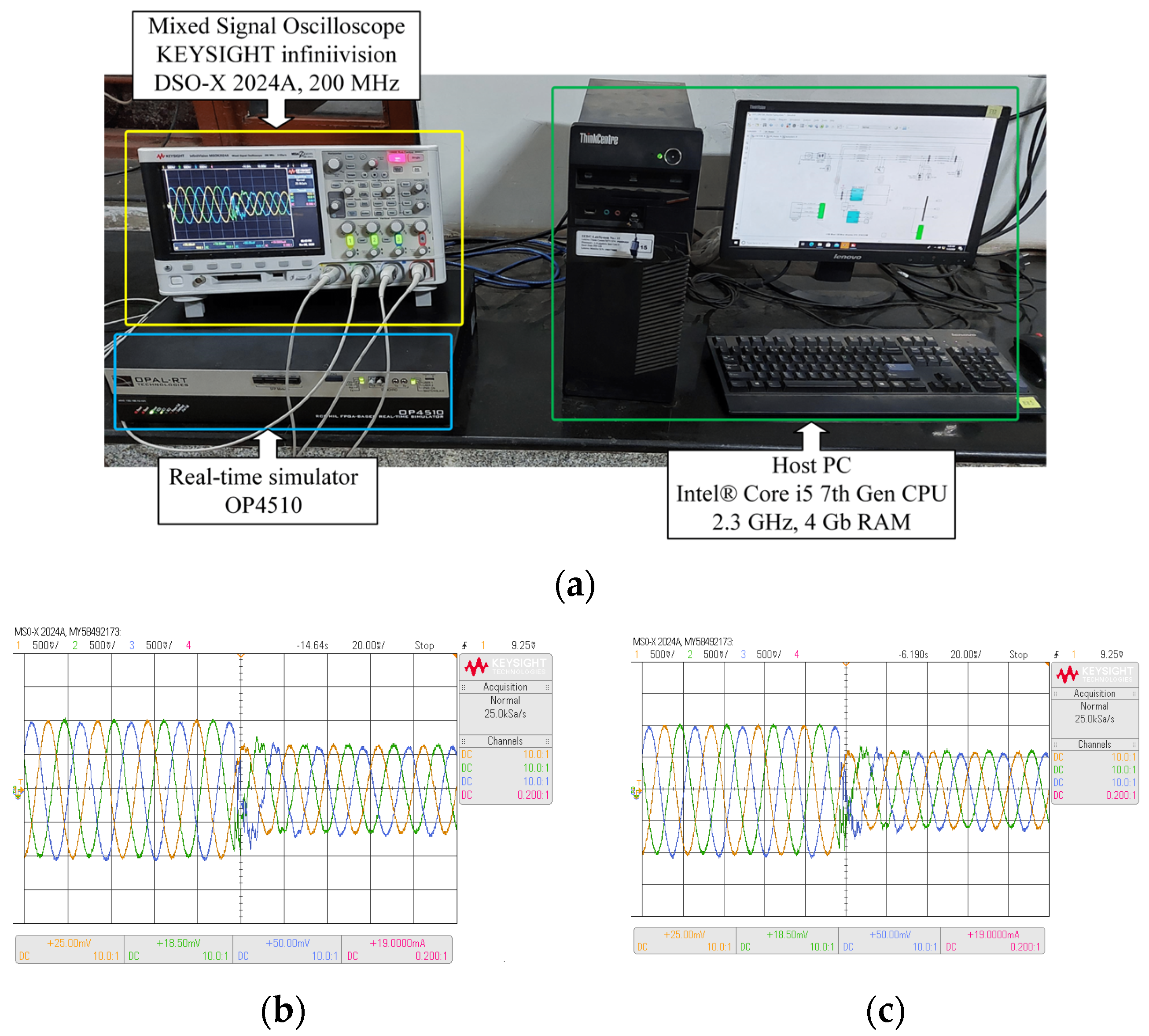
• The real-time validation of EMD-based FLM with Opal-RT is presented.

The organization of the paper is as follows. Section 2 presents an overview of different signal decomposition techniques which are utilized to develop FLMs. Section 3 consists of a description of the system considered for simulation study. In Section 4, the methodologies adopted to develop different FLMs are described. Numerical test cases and respective results are presented in Section 5. In Section 6, critical findings regarding characteristics of developed FLMs are pointed out. Conclusions drawn on the basis of research findings are presented in the final section.

2. Overview of Signal Decomposition Techniques

2.1. Intrinsic Time Decomposition (ITD)

ITD was introduced as an effective tool for time-frequency-energy analysis [26]. This technique offers advantages such as simpler calculations, precise information, and real-time applicability. ITD is used to decompose a signal into a sum of principle rotation components (PRCs). To mathematically understand the process adopted in ITD, for a signal $S_m$, there is an operator $\mathsf{\Phi }$ which decomposes the signal $S_m$ into a baseline signal and a residual signal such as the residual, considered as the PRC of signal $S_m$. It is expressed as

$$S_m=\mathsf{\Phi }{S}_m+\left(1-\mathsf{\Phi }\right)S_m=B_m+P_m$$

(1)

where $B_m=\mathsf{\Phi }{S}_m$ is the baseline signal and $P_m=\left(1-\mathsf{\Phi }\right)S_m$ is the proper rotation.

Let $B_m\in \left(0,{\tau }_n\right)$ and $P_m\in \left(0,{\tau }_n\right)$, where ${\tau }_n,\left(n=1, 2,\dots \right)$ represents local minima and maxima of the signal $S_m$. The signal $S_m$ is in the range $\left[0,{\tau }_{n+2}\right]$. Between successive extrema, the operator $\mathsf{\Phi }$ in the interval $\left[{\tau }_n,{\tau }_{n+1}\right]$ is expressed as

$$S_m=B_m=B_n+\left(\frac{B_{n+1}-B_n}{S_{n+1}-S_n}\right)\left(S_m-S_n\right), m\in \left[{\tau }_n,{\tau }_{n+1}\right]$$

(2)

where,

$$B_{n+1}=\alpha \left[S_n+\left(\frac{{\tau }_{n+1}-{\tau }_n}{{\tau }_{n+2}-{\tau }_n}\right)\left(S_{n+2}-S_n\right)\right]+\left(1-\alpha \right)S_{n+1}$$

(3)

and $0<\alpha <1$ (generally $\alpha$ is set equal to 0.5). After the estimation of baseline signal $B_m$, the proper rotating extracting operator $\mathsf{\Theta }$ is calculated as

$$\mathsf{\Theta }{S}_m=\left(1-\mathsf{\Phi }\right)S_m=P_m=S_m-B_m$$

(4)

The above process is repeated considering baseline signals as input signals to next-level decomposition until a monotonic trend is obtained.

2.2. Empirical Mode Decomposition (EMD)

EMD is a signal processing technique used for time-frequency analysis. It decomposes any signal into numerous intrinsic mode functions (IMFs) and a residual [27]. Primarily, this technique iteratively decomposes the signal $S_m$ into several IMFs and a residual by involving a sifting process. The involved decomposition is represented as

$$S_m={{\displaystyle \sum }}_{r=1}^R{I}_m^r+W_m^R$$

(5)

where $I_m^r$ is the $r$th IMF and $W_m^R$ denotes residual calculated after iteration ends.

Since this method iteratively involves the sifting process, therefore, a termination criterion is required to end the process. The termination is achieved by a sift relative tolerance measure ${ϵ}_m$ represented as

$${ϵ}_m=\frac{{\left({ϵ}_m^{previous}-{ϵ}_m^{current}\right)}^2}{{\left({ϵ}_m^{previous}\right)}^2}$$

(6)

where ${ϵ}_m^{previous}$ and ${ϵ}_m^{current}$ are previous and current values of relative tolerance, respectively. The described sifting process ends when ${ϵ}_m$ is found to be less than considered tolerance.

An energy ratio criterion (ERC) is utilized as a stopping criterion for the depth of decomposition. Mathematically, ERC defined $r$th IMF is represented as

$$E_m=10{\log }_{10}\frac{{(S_m^r)}^2}{{(A_m^r)}^2}$$

(7)

where ${(S_m^r)}^2$ and ${(A_m^r)}^2$ are the energy of the signal obtained at start of sifting process and average value of envelope energy, respectively. The stopping criterion for the level of decomposition is the condition when current $E_m$ is found to be greater than the maximum defined $E_m$. The detailed algorithm of EMD process is found in [4].

2.3. S-Transform (ST)

ST is predominantly developed as a technique to incorporate correction of phase in continuous wavelet transform (CWT) [28]. The CWT of a signal $S_m$ is expressed as

$$W_{\tau ,d}={\int }_{-\infty }^{\infty }\mathrm{}{S}_m{w}_{m-\tau ,d}dm$$

(8)

where $w_{m-\tau ,d}$ is a scaled version of mother wavelet and $d$ is the dilation which controls the resolution. ST of the signal $S_m$ is basically a CWT with a certain mother wavelet scaled up by a phase factor. It is represented as

$$S{T}_{\tau ,F}=e^{i2\pi F\tau }{W}_{\tau ,d}$$

(9)

where the mother wavelet is expressed as

$$w_{\tau ,F}=\frac{\left|F\right|}{\sqrt{2\pi }}{e}^{-\frac{m^2{F}^2}{2}}{e}^{-i2\pi Fm}$$

(10)

Here, the dilation factor $d=\frac{1}{F}$. Thus, ST can be written explicitly as

$$S_{\tau ,F}={\int }_{-\infty }^{\infty }\mathrm{}{S}_m\frac{\left|F\right|}{\sqrt{2\pi }}{e}^{-\frac{(\tau -m{)}^2{F}^2}{2}}{e}^{-i2\pi Fm}dm$$

(11)

The detailed explanation of ST is given in [28].

2.4. Estimation of Signal Parameters via Rotational Invariance Technique (ESPRIT)

ESPRIT is a subspace parametric method and was initially introduced to detect the direction of arrival [29]. Basically, ESPRIT divides a signal into subspace matrices of signal and noise. Consider a signal $S\left[m\right]$ of length $M$ in discrete form as

$$S\left[m\right]={{\displaystyle \sum }}_{r=1}^R{\psi }_{r}u\left(f_r\right)e^{j2\pi m{f}_r}+w\left[m\right]=U{\mathsf{\Theta }}^m\psi +w\left[m\right]$$

(12)

where $U$ is M$\times$R matrix constructed from frequency vectors $u\left(f_r\right)={[1 e^{j2\pi f_r} e^{j4\pi f_r}\dots e^{j2\pi \left(R-1\right)f_r}]}^T$ of length $M$ for each $R$ frequencies and $U=\left[u\left(f_1\right) u\left(f_2\right) \dots u\left(f_r\right)\right]$. $\psi$ is a vector containing amplitudes of each ${\psi }_r$. $\mathsf{\Theta }$ is a diagonal matrix composed of shifted phases between two consecutive samples of signal $S\left[m\right]$. $w\left[n\right]$ is the vector of noise components.

$$\mathsf{\Theta }=\left[\begin{array}{llll}{\theta }_1\hfill & 0\hfill & \cdots \hfill & 0\hfill \\ 0\hfill & {\theta }_2\hfill & \cdots \hfill & 0\hfill \\ ⋮\hfill & ⋮\hfill & \ddots \hfill & ⋮\hfill \\ 0\hfill & 0\hfill & \cdots \hfill & {\theta }_r\hfill \end{array}\right]=\left[\begin{array}{llll}{e}^{j2\pi f_1}\hfill & 0\hfill & \cdots \hfill & 0\hfill \\ 0\hfill & e^{j2\pi f_2}\hfill & \cdots \hfill & 0\hfill \\ ⋮\hfill & ⋮\hfill & \ddots \hfill & ⋮\hfill \\ 0\hfill & 0\hfill & \cdots \hfill & e^{j2\pi f_r}\hfill \end{array}\right]$$

(13)

From (13), it is noted that $\mathsf{\Theta }$ is a rotation matrix utilized by ESPRIT to determine frequency extracts. Consider, two sub-windows $s_{M-1}\left[m\right]$ and $s_{M-1}\left[m+1\right]$ of length $M-1$ which are over-lapping with each other are present, then the signal $s\left[m\right]$ is represented as

$$s\left[m\right]=\left[\begin{array}{l}{s}_{M-1}\left[m\right]\hfill \\ s_{M-1}\left[m+M-1\right]\hfill \end{array}\right]=\left[\begin{array}{l}{s}_{M-1}\left[m\right]\hfill \\ s_{M-1}\left[m+1\right]\hfill \end{array}\right]$$

(14)

Since $s_{M-1}\left[m\right]$ is sub-window of $s\left[m\right]$ of length $M-1$, it can be mathematically shown as

$$s_{M-1}\left[m\right]=V_{M-1}{\Theta }_m\psi$$

(15)

From (15), two sub-window matrices are formed as

$$V_1=V_{M-1}{\Theta }_m$$

(16)

$$V_2=V_{M-1}{\Theta }_{m+1}$$

(17)

From the above sub-window matrices, a matrix $U$ is obtained as

$$U=V_1\backslash V_2$$

(18)

Once matrix $U$ is obtained, a left-hand eigenvalue problem can be solved as

$$z=eig\left(U\right)$$

(19)

The residue matrix $Y$ is computed after solving eigenvalue problems as

$$Y=z^{†}s\left[m\right]$$

(20)

where $†$ represents the pseudo-inverse. The signal parameters can be obtained from the above equations.

2.5. Teager Energy of a Signal

To calculate the energy of the signals, the Teager energy operator was introduced in [30]. If a signal $s\left[m\right]$ is in its discrete form, then the energy of the signal $E_s\left[m\right]$ is calculated as

$$E_s\left[m\right]=s^2\left[m\right]-s\left[m+1\right]s\left[m-1\right]$$

(21)

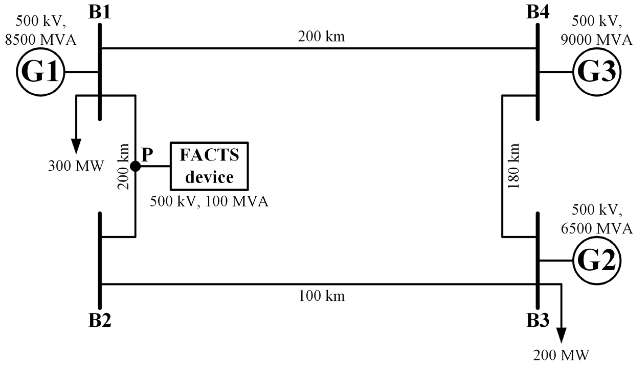
3. System under Study

A three-machine system, as shown in Figure 1, was used in this study for simulation. A 500 kV transmission network was modeled. A 500 kV, 100 MVA FACTS device was connected at the middle of the line B1–B2, with a total length of 200 km at point P. Three generators, G1 (8500 MVA), G2 (6500 MVA), and G3 (9000 MVA), were installed at terminals B1, B3, and B4, respectively. Two loads, 300 MW and 200 MW, were present at terminal B1 and B3, respectively. The parameters of the lines are taken as distributed model. The inductance $L$ of the line is 0.0009337 H/km, while the capacitance $C$ of the line is 12.74 × 10⁻⁹ F/km. Thus, the wave speed $v=\frac{1}{\sqrt{LC}}$ is equal to 2.8994 × 10⁵ km/s. The simulation model is developed on MATLAB platform.

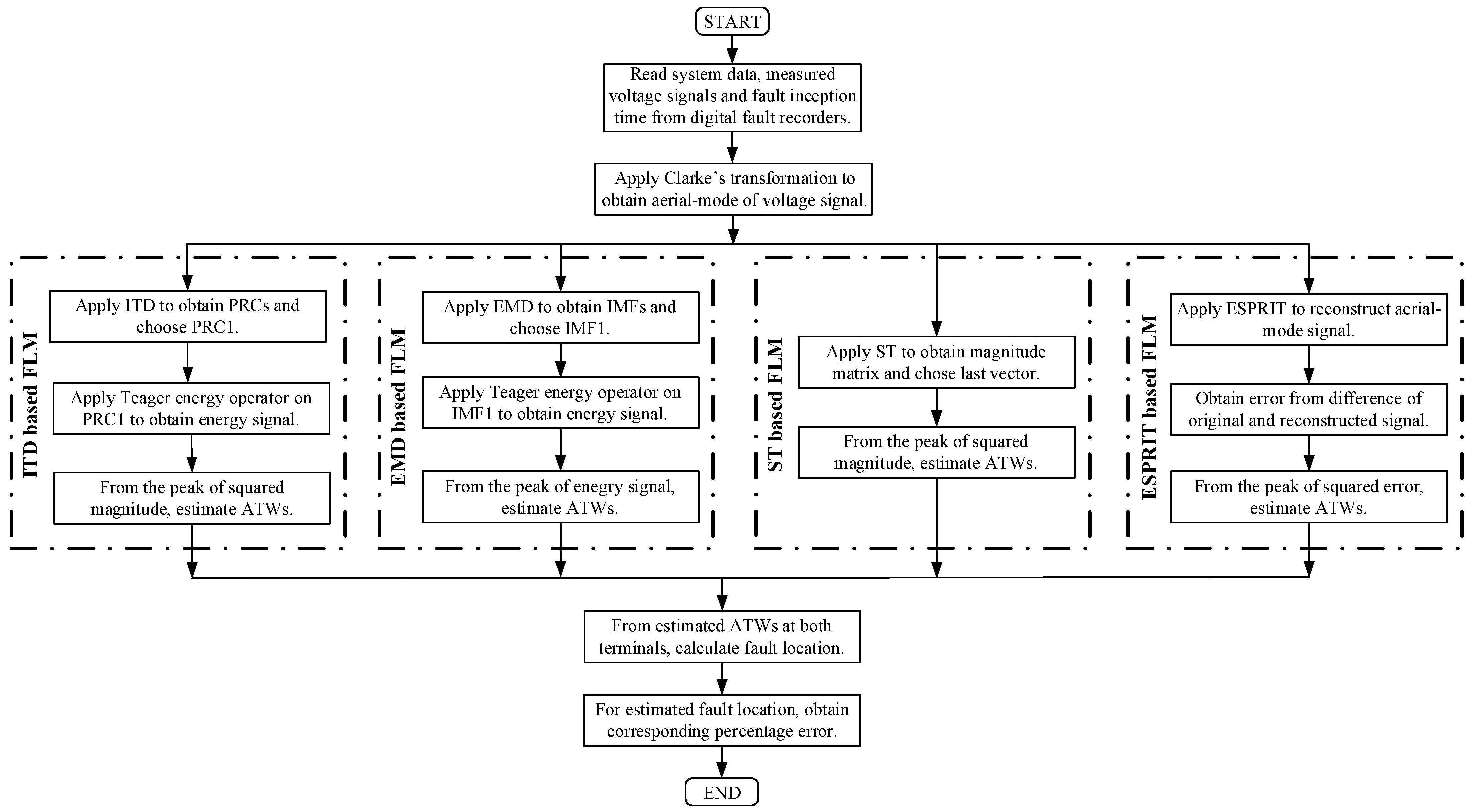
4. Development of Fault Location Methods

Traveling wave-based FLMs are based on estimation of ATWs at the terminals of the lines and their utilization in calculating the location of the faults. Therefore, it can be mentioned that the prime difference in all traveling wave-based FLMs lies in the technique adopted for detection and estimation of ATWs. The basic steps involved in traveling wave-based FLMs are mentioned below.

• Consider a transmission line B1–B2, as shown in Figure 1, on which a double line to ground fault occurs at 111.30 km from bus B1. Fault inception time is 0.3 s. From the traveling wave theory, the waves originate from the point of fault and travel towards terminal B1 and B2 and will get terminated. The instantaneous voltage signals measured at terminal B1 and B2 are recorded.
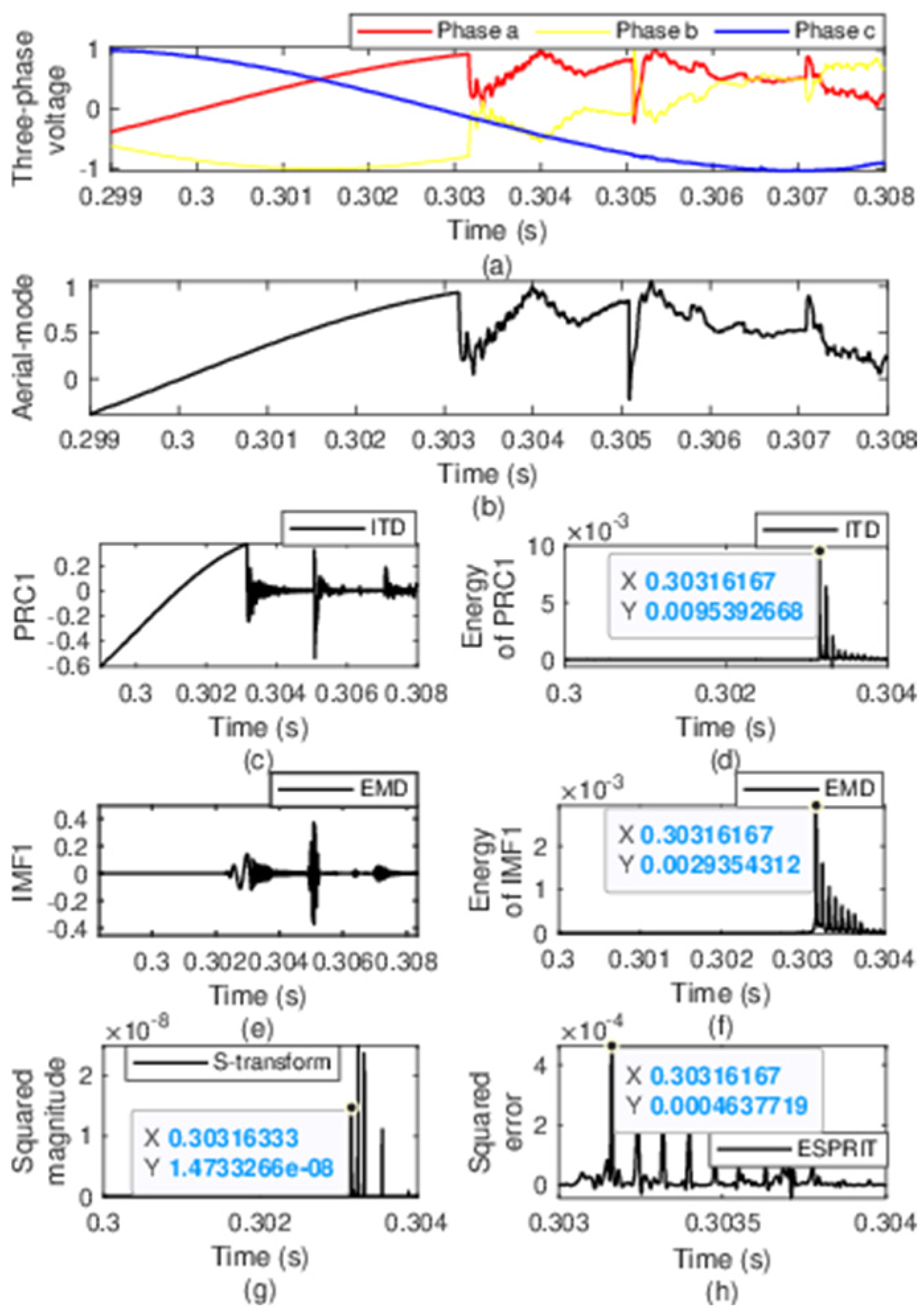
• The voltage signals are decoupled using Clarke’s transformation and modal signals are obtained.
• Aerial-mode of the signals are selected and decomposed using any signal processing techniques.
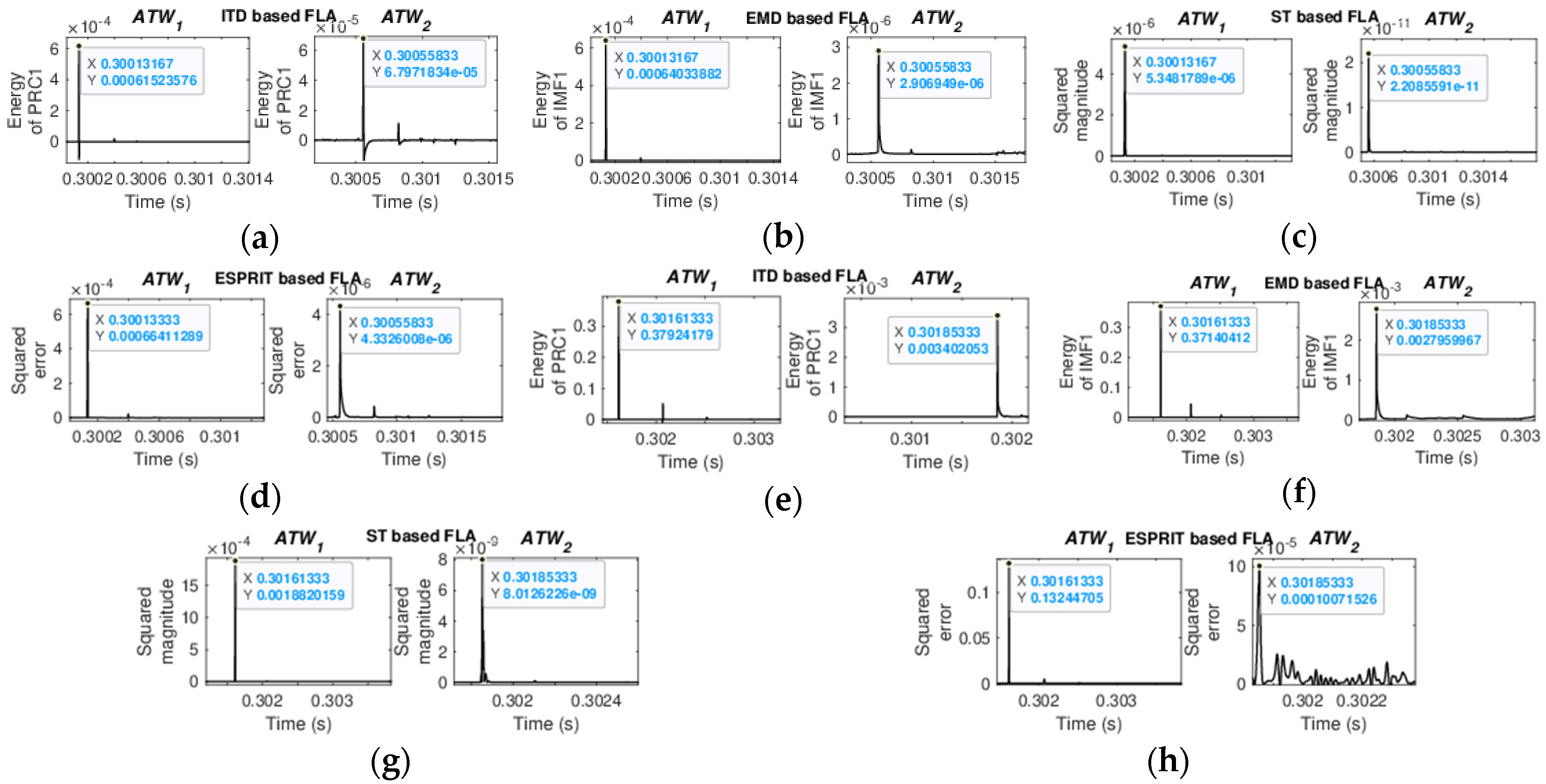
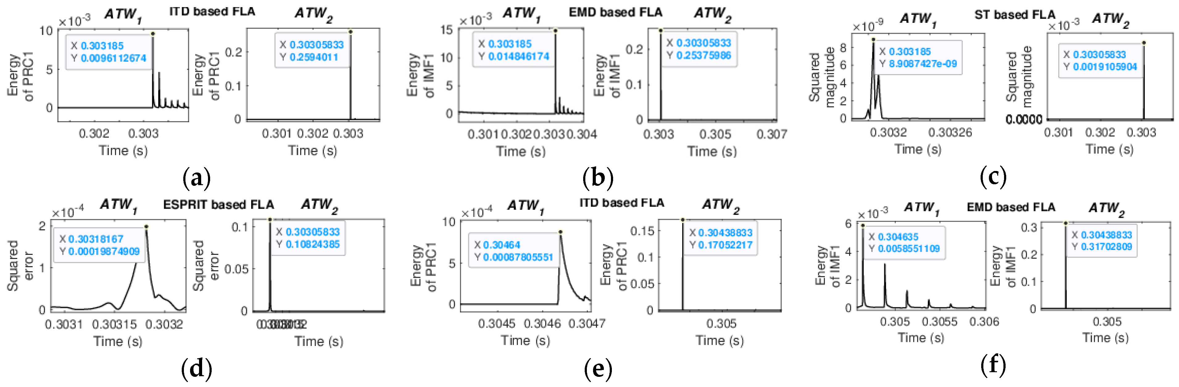
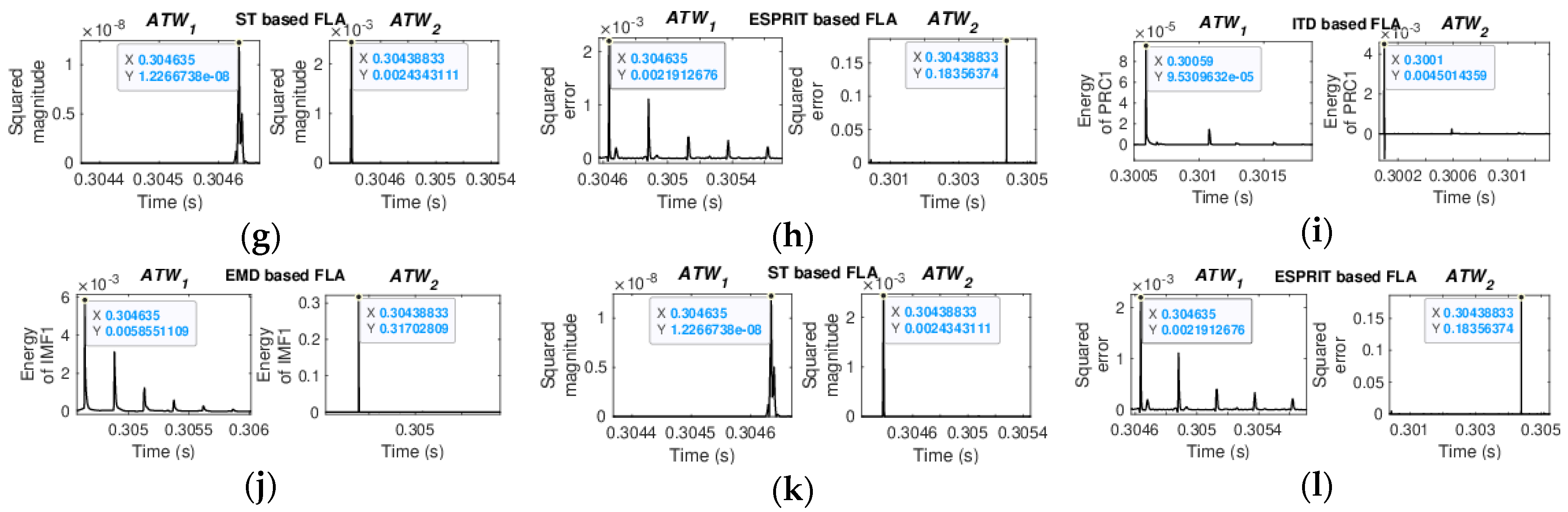
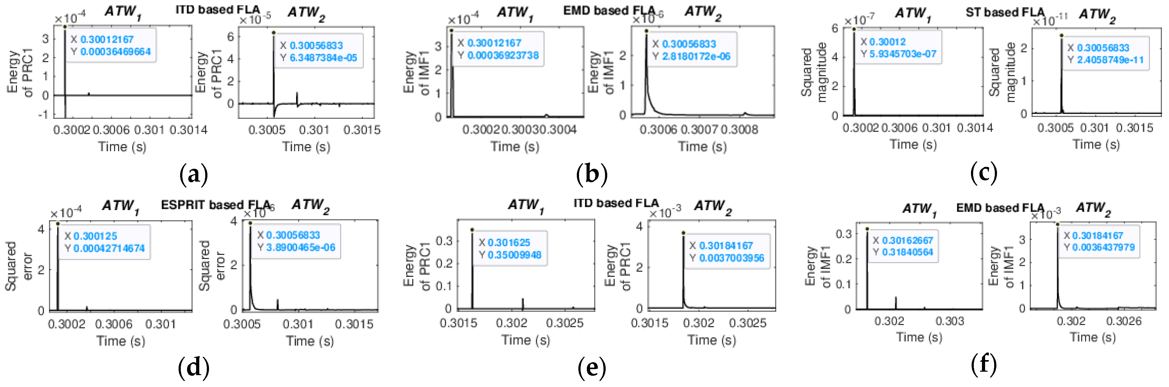
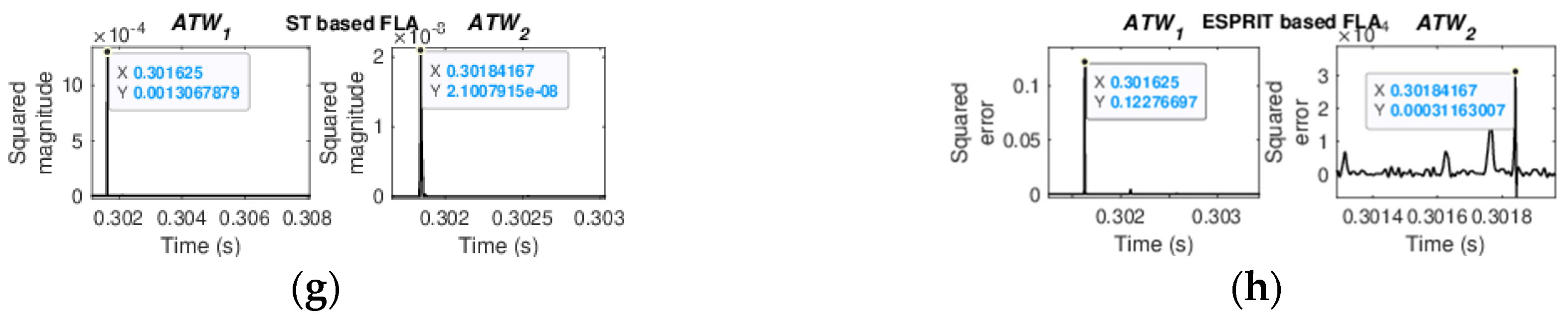
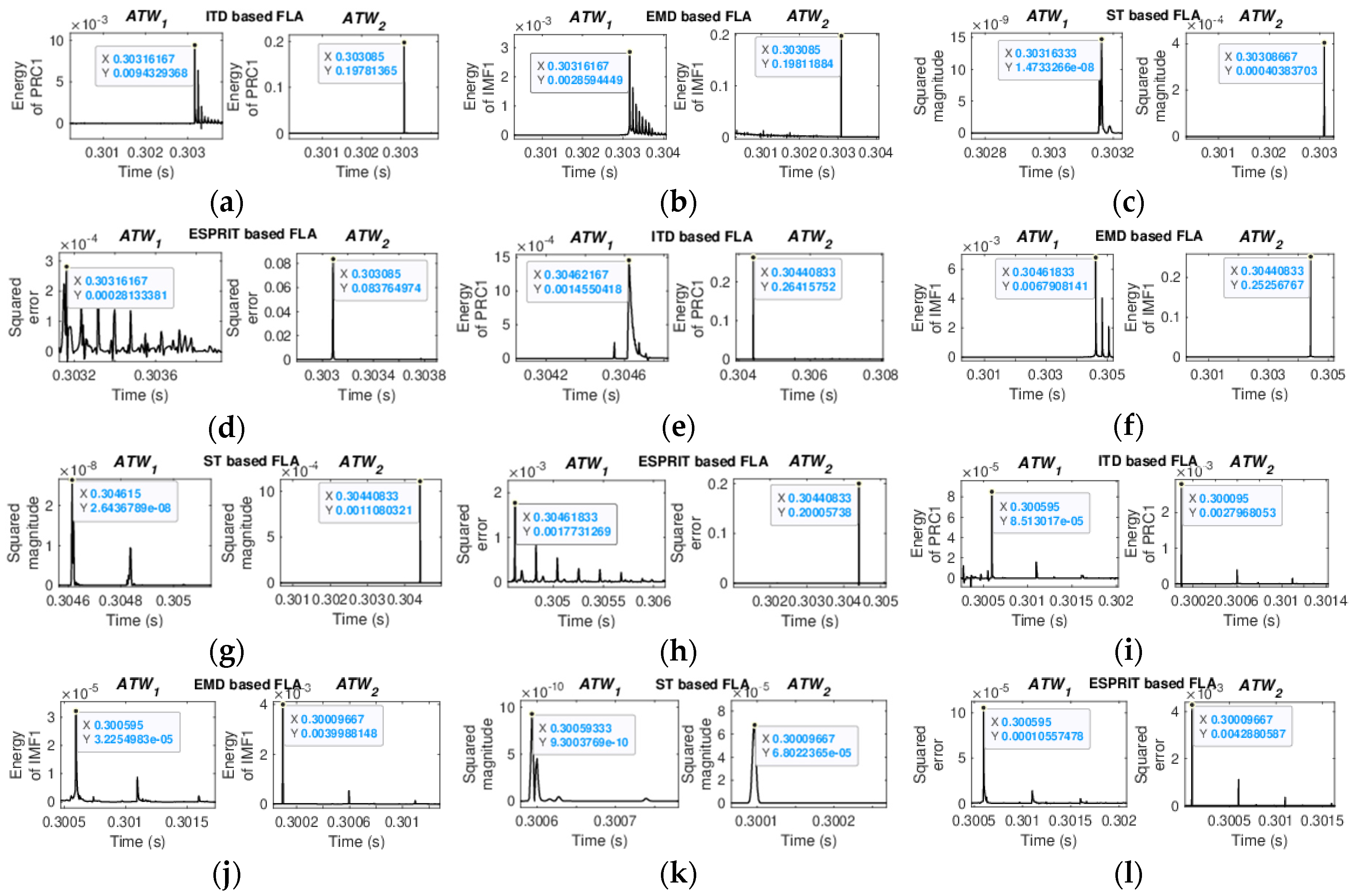
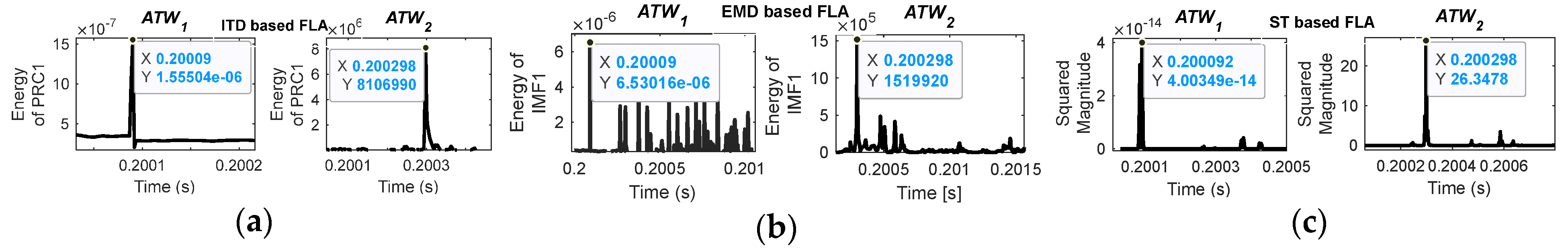
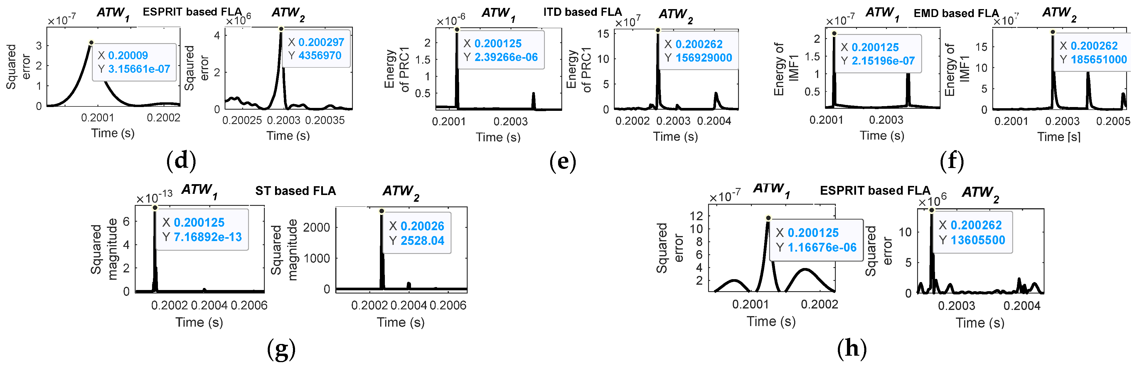
• From the decomposed signals, ATWs are detected and estimated. For ITD and EMD-based FLMs, Teager energy is calculated from decomposed signals, and the instant peak of energy signals is considered as ATW. For ST-based FLM, the instant of peak of squared magnitude was utilized to estimate ATW, whereas for ESPRIT-based FLM, the instant peak of squared error was used to estimate ATW. The estimated ATWs at the bus B1 and B2 are $AT{W}_1$ and $AT{W}_2$, respectively.
• The distance of fault point from bus B1 is calculated by the expression given as follows.

  $$EFL=\frac{1}{2}\left(TL-v\left(AT{W}_2-AT{W}_1\right)\right)$$

  (22)

  where $TL$ is the total length of the transmission line in km and $v$ is the wave speed in km/s.
• The percentage error for obtained $EFL$ is calculated in the following manner.

  $$\%Error=\frac{\left|AFL-EFL\right|}{TL}\times 100$$

  (23)

  where $AFL$ is the actual location of fault in km.

4.1. ITD-Based FLM

In this method, the detection of arrival waves and estimation of ATWs are carried out by decomposing aerial-mode voltage signals by ITD techniques. The instant of peak of PRC1 obtained by decomposition of modal signals via ITD was used in estimation of ATWs [1]. This method accurately estimates ATWs. However, in this study, an ITD-based FLM is modified by calculating the energy of PRC1 using (21). The appearance time of crest of the energy signal is considered as ATWs. This modification improves the accuracy of ITD-based FLM.

4.2. EMD-Based FLM

In this method, the EMD technique is used to decompose the modal signals to obtain IMFs. As proposed in [4], the instant of sharp peak of IMF1 obtained after decomposing aerial-mode signals via EMD is used to determine ATWs. However, it is difficult to observe sharp peak always. Therefore, in this work, the instant of peak of energy of IMF1 calculated using (21) was used to determine the ATW. This modification increases the efficiency of EMD-based FLM.

4.3. ST-Based FLM

ST-based FLM determines ATWS by observing the peak of squared magnitude of the aerial-mode signals decomposed via ST [31]. The instant of peak of squared magnitude is considered as ATW. This technique is used here without any further modification.

4.4. ESPRIT-Based FLM

In this method, the three-phase instantaneous voltage signals are reproduced with the ESPRIT method and the aerial-mode signals are obtained for both original and reconstructed signals [2]. An error signal is determined from the difference of modal signals (calculated from original and reproduced signals). The appearance of crest of squared error signals is considered as ATW [2].

An illustrative example showing the estimation of ATW by ITD, EMD, ST, and ESPRIT-based FLMs is presented in Figure 2. The measured voltage signals at bus B1 are depicted in Figure 2a. Aerial-mode signal obtained via Clarke’s transformation is depicted in Figure 2b. ITD is used to decompose the aerial-mode signal and PRC1 is obtained. Subsequently, the energy of the PRC1 signal is calculated. In Figure 2c,d, PRC1 and its energy signal are shown, respectively. Similarly, IMF1 obtained via EMD and its energy signal are presented in Figure 2e,f, respectively. The instant of peak of energy signal is ATW. In Figure 2g, the squared magnitude plot obtained from ST-based FLM is depicted, and ATW is determined from the instant of peak of the signals. The squared error signal for ESPRIT-based FLM is presented in Figure 2h. In a similar way, the time observed at maximum value of squared error signals is used as ATW. The flowchart of FLMs is illustrated in Figure 3.

5. Numerical and Simulation Results

To critically compare ITD, EMD, ST, and EPSRIT-based FLMs for locating faults in FACTS-compensated systems, several cases of different scenarios are considered for the studied system. A 100 MVA UPFC is installed at mid-point of 500 kV and 200 km line B1-B2. Three different cases of series compensation (UPFC operating as SSSC in voltage injection mode), shunt compensation (UPFC operating as STATCOM in Var control mode), and series-shunt compensation (UPFC operating in power control mode) are considered in this work. Several tests of different types of faults, varying fault resistances (FRs) and fault inception angles (FIAs), and high resistance faults are carried out in the aforementioned cases. During all simulations, the faults are initiated on the line at 0.3 s. A high sampling frequency (600 kHz) is used to sample measured signals for improved accuracy of FLMs. The rated frequency of the system used for simulation is 60 Hz. All simulations are carried out in a MATLAB environment. Following subsections presents the results for the considered cases.

5.1. Performance under Series Compensation

In this case, UPFC operates as SSSC in voltage injection mode.

Table 1. Performance under series compensation (mid-point connected SSSC).

	Scenario	Different Fault Conditions				ITD-Based FLM		EMD-Based FLM		ST-Based FLM		ESPRIT-Based FLM
		Fault Type	AFL (km)	FR $\left(\mathsf{\Omega }\right)$	FIA (deg.)	EFL (km)	%Error	EFL (km)	%Error	EFL (km)	%Error	EFL (km)	%Error
Before SSSC	1.	AG	38.30	0.01	0	38.1471	0.0765	38.1471	0.0765	38.1471	0.0765	38.3877	0.0439
	2.	AB	65.40	0.1	30	65.2072	0.0964	65.2072	0.0964	65.2072	0.0964	65.2072	0.0964
After SSSC	3.	ABG	118.20	1	60	118.3633	0.0817	118.3633	0.0817	118.3633	0.0817	117.8806	0.1597
	4.	ABC	135.60	10	90	136.4846	0.4423	135.7597	0.0799	135.7597	0.0799	135.7597	0.0799
	5.	ABCG	170.80	100	0	171.0353	0.1177	171.0353	0.1177	171.0353	0.1177	171.0353	0.1177

Bold-faced data are minimum values.

lists the considered fault scenarios. A total of five test scenarios are simulated, out of which two fault scenarios are initiated before SSSC and three after SSSC location. Four different FLMs are used to determine ATWs for simulated scenarios. The estimated ATWs from different FLMs for tabulated scenarios are illustrated in Figure 4 and Figure 5. In Figure 4, estimated ATWs are depicted for fault scenarios before SSSC, while Figure 5 shows estimated ATWs for fault scenarios after SSSC. The obtained results are tabulated in Table 1. From the results, minimum percentage errors are obtained from EMD, ST, and ESPRIT-based FLMs for four different scenarios. Moreover, the percentage errors obtained from all methods for different scenarios were found to be less than 1%, which is well within the acceptable limit of 1%. Therefore, it can be noted that performance of all four methods is satisfactory regarding the location of faults in series-compensated systems. It is quite noticeable that the presence of SSSC in the fault loop does not affect the accuracy of FLMs. In other words, it can be mentioned as the developed FLMs are robust towards the existence of SSSC in the fault loop.

5.2. Performance under Shunt Compensation

In this case, UPFC operates as STATCOM in Var control mode. Five different fault scenarios were simulated to validate the effective performance of four different FLMs for shunt-compensated systems. The fault scenarios are listed in

Table 2. Performance under shunt compensation (mid-point connected STATCOM).

	Scenario	Different Fault Conditions				ITD-Based FLM		EMD-Based FLM		ST-Based FLM		ESPRIT-Based FLM
		Fault Type	AFL (km)	FR $\left(\mathsf{\Omega }\right)$	FIA (deg.)	EFL (km)	%Error	EFL (km)	%Error	EFL (km)	%Error	EFL (km)	%Error
Before STATCOM	1.	AG	35.50	0.01	0	35.2477	0.1262	35.2477	0.1262	35.0056	0.2472	35.7304	0.1152
	2.	AB	68.80	0.1	30	68.5894	0.1053	68.8314	0.0157	68.5894	0.1053	68.5894	0.1053
After STATCOM	3.	ABG	115.90	1	60	115.9467	0.0233	115.9467	0.0233	116.1874	0.1437	115.9467	0.0233
	4.	ABC	132.10	10	90	133.3431	0.6216	131.8934	0.1033	131.8934	0.1033	132.3762	0.1381
	5.	ABCG	168.50	100	0	168.6201	0.0600	168.6201	0.0600	168.6201	0.0600	168.6201	0.0600

Bold-faced data are minimum values.

. ATWs determined from FLMs for the first two cases are shown in Figure 6. Figure 7 depicts the estimated ATWs for three scenarios after STATCOM. The fault location and corresponding percentage errors are calculated for all scenarios from different methods and are tabulated in Table 2. An observation of the obtained results suggests that ITD and ESPRIT-based FLMs are better than EMD and ST-based FLMs. It should be noted here that the modification in ITD-based FLM improves its accuracy. Moreover, all methods perform well, since the percentage errors are less than targeted value of 1%. In this case, it can be noted that the effectiveness of FLMs remains unaffected in the presence of STATCOM in the fault loop.

5.3. Performance under Series-Shunt Compensation

In this case, UPFC is operating in power control mode. The fault scenarios are listed in

Table 3. Performance under series-shunt compensation (mid-point connected UPFC).

	Scenario	Different Fault Conditions				ITD-Based FLM		EMD-Based FLM		ST-Based FLM		ESPRIT-Based FLM
		Fault Type	AFL (km)	FR $\left(\mathsf{\Omega }\right)$	FIA (deg.)	EFL (km)	%Error	EFL (km)	%Error	EFL (km)	%Error	EFL (km)	%Error
Before UPFC	1.	AG	40.20	0.01	0	40.0781	0.6090	40.0781	0.609	40.0781	0.6090	40.3202	0.0601
	2.	AB	70.40	0.1	30	70.5218	0.0609	70.5218	0.0609	71.0060	0.3030	70.7639	0.1820
After UPFC	3.	ABG	111.30	1	60	111.1148	0.0926	111.1148	0.0926	110.8235	0.2383	111.1148	0.0926
	4.	ABC	130.60	10	90	130.9279	0.1639	130.9515	0.1758	129.9609	0.3195	130.4437	0.0782
	5.	ABCG	172.50	100	0	172.4850	0.0075	172.2429	0.1285	172.0008	0.2496	172.2429	0.1285

Bold-faced data are minimum values.

. The estimated ATWs for considered fault scenarios are illustrated in Figure 8 and Figure 9. In Figure 8, ATWs are shown for scenarios before UPFC. Fault scenarios after UPFC are depicted in Figure 9. EFLs and respective percentage errors are tabulated in Table 3. From the results, it is observed that EMD-based FLM is producing minimum percentage errors for three scenarios. However, ITD and ESPRIT-based FLMs are found to be performing better than ST-based FLM. The overall performance of all methods is acceptable. This case further reveals that the presence of UPFC in the fault loop does not affect the performance of developed FLMs. Consequently, it can be concluded that EMD and ITD-based FLMs perform better after the modification proposed in this work.

5.4. Performance under UPFC Compensation in Two-Area Four-Machine Kundur 11-Bus Test System

In this case, the Kundur two-area four-machine 11-bus test system was considered, in which line 7–8 is compensated with a mid-point connected UPFC as shown in Figure 10. UPFC is operating in power control mode. For simulations, a three-phase to ground fault was initiated at 0.2 s on line 7–8. The fault scenarios are listed in

Table 4. Performance under series-shunt compensation in two-area four-machine Kundur 11-bus test system.

	Scenario	Different Fault Conditions				ITD-Based FLM		EMD-Based FLM		ST-Based FLM		ESPRIT-Based FLM
		Fault Type	AFL (km)	FR $\left(\mathsf{\Omega }\right)$	FIA (deg.)	EFL (km)	%Error	EFL (km)	%Error	EFL (km)	%Error	EFL (km)	%Error
Before UPFC	1.	AG	25.30	0.01	0	25.3140	0.0127	25.3140	0.0127	25.5515	0.2286	25.5040	0.1855
	2.	AB	35.40	0.1	30	35.5260	0.1145	35.5260	0.1145	35.7635	0.3304	35.5260	0.1145
After UPFC	3.	ABG	75.60	1	60	76.1364	0.4876	76.1364	0.4876	75.8989	0.2717	76.6588	0.9626
	4.	ABC	65.70	10	90	66.6843	0.8949	66.1619	0.4199	65.9719	0.2472	65.9719	0.2472
	5.	ABCG	85.90	100	0	86.3484	0.4985	86.3484	0.4985	77.7988	7.2738	69.6767	14.6575

Bold-faced data are minimum values.

. The estimated ATWs for considered fault scenarios are illustrated in Figure 11 and Figure 12. In Figure 11, ATWs are shown for scenarios before UPFC. Fault scenarios after UPFC are depicted in Figure 12. EFLs and respective percentage errors are tabulated in Table 4. From the results, it is observed that EMD and ITD-based FLM produce minimum percentage errors for three scenarios out of five (highlighted in bold), while ST and ESPRIT-based FLMs produce minimum percentage errors two times (highlighted in bold). For scenario 5, ST and ESPRIT-based FLMs fail to produce acceptable results (highlighted in yellow). Therefore, it can be concluded that ST and ESPRIT-based FLMS may produce inaccurate results for large practical power systems. Further, it is noted that EMD and ITD-based FLMs perform better after the modification proposed in this work.

5.5. Critical Discussion

From the results of the aforementioned three cases, it can arguably be mentioned that all methods are performing satisfactorily. However, for a few of the case scenarios (scenarios 1, 3, and 5 of case 1, scenarios 2, 3, and 4 of case 2, and scenarios 2, 3, and 4 of case 3), EMD and ESPRIT-based FLMs are efficiently performing in comparison to ITD and ST-based FLMs. The critical points from the above discussion are presented below.

• The modifications proposed in this work for ITD and EMD-based FLMs improve their respective performance regarding fault locations in FACTS-compensated systems.
• EMD performs better on most occasions.
• ST-based FLM is found to estimate the location with some error of around 1%.
• ESPRIT-based FLM involves complex methodology in estimating ATWs compared to other three, since reconstruction of signals is required with the help of matrix computations.
• For large practical power systems, EMD and ITD-based FLMs perform better, whereas ST and ESPRIT-based FLMs failed to perform accurately for one test scenario.
• EMD-based FLM performs efficiently with real-time signals.

5.6. Real-Time Validation of Proposed FLM

From the critical discussion in the above section, it was found that EMD-based FLM performs better on most occasions in comparison to others. Therefore, the performance of this method will be validated with real-time data obtained from Opal-RT in this section. The experimental set-up of the test is shown in Figure 13a. The set-up consists of a host computer, a real-time simulator (OP4510), and a mixed signal oscillator (MSO). For real-time data generation, the three-generator system with UPFC is modeled in RT-Lab software and the analog voltage signals of the terminals are recorded in mixed storage oscilloscope (MSO). For simulation, a three-phase to ground fault is initiated on line B1–B2 at 150 km away from bus B1 of studied system at time 0.2 s. Figure 13b,c illustrate the three-phase instantaneous voltage signals recorder by MSO at bus B1 and bus B2, respectively. These signals are used by EMD-based FLM to estimate ATWs at the buses in MATLAB environment. Figure 13d,e show the estimated ATWs, i.e., ATW₁ and ATW₂ obtained via EMD-based FLM, respectively. The fault location and corresponding percentage error is calculated in the following manner.

$$EFL=\frac{200-2.8994\times {10}^5\left(0.200172-0.200518\right)}{2}=150.2563$$

(24)

$$\% Error=\frac{\left|150-150.2563\right|}{200}\times 100=0.1281$$

(25)

From the above calculation, the percentage error is found to be within an acceptable limit of 1%. This certifies the efficient performance of EMD-based FLM.

6. Conclusions

This work presents a performance comparison of traveling wave aided FLMs-based on ITD, EMD, ST, and ESPRIT techniques for a system compensated with FACTS devices. Fault localization is achieved from the knowledge of estimated ATWs. In the case of ITD and EMD-based FLMs, ATWs are determined from the crest of energy signals of the first PRC and first IMF, respectively. For simulation, UPFC operates as SSSC in voltage injection mode, as STATCOM in Var control mode, and as UPFC in power control mode. The performance of all FLMs is investigated for system operating under different scenarios. Cases of varying types of faults, varying FRs and FIAs, and high resistance faults are considered. The simulation results ascertain satisfactory performance of presented FLMs. It is worth noting that the accuracy of EMD-based FLM is more than others for most cases. Further, real-time validation of EMD-based FLM signifies its efficient performance. It is noticeable here that the effect on accuracy of fault location due to the presence of FACTS devices in the fault loop is minimal with the aforementioned traveling wave-based FLMs.

References

1. Mishra, S.; Gupta, S.; Yadav, A. Intrinsic time decomposition based fault location scheme for unified power flow controller compensated transmission line. Int. Trans. Electr. Energy Syst. 2020, 30, e12585. [Google Scholar] [CrossRef]
2. Mishra, S.; Gupta, S.; Yadav, A. A novel two-terminal fault location approach utilizing traveling-waves for series compensated line connected to wind farms. Electr. Power Syst. Res. 2021, 198, 107362. [Google Scholar] [CrossRef]
3. Fan, X.-Q.; Zhu, Y.-L.; Lu, W.-F. Traveling wave based fault location for transmission lines based on EMD-TEO. Power Syst. Prot. Control 2012, 40, 8–12+17. [Google Scholar]
4. Mishra, S.; Gupta, S.; Yadav, A. Empirical mode decomposition assisted fault localization for UPFC compensated system. In Proceedings of the 2020 21st National Power Systems Conference (NPSC), Gandhinagar, India, 17–19 December 2020; pp. 1–6. [Google Scholar]
5. Abdelaziz, A.; Ibrahim, A.; Mansour, M.; Talaat, H. Modern approaches for protection of series compensated transmission lines. Electr. Power Syst. Res. 2005, 75, 85–98. [Google Scholar] [CrossRef]
6. Abdelaziz, A.; Mekhamer, S.; Ezzat, M. Fault location of uncompensated/series-compensated lines using two-end synchronized measurements. Electr. Power Compon. Syst. 2013, 41, 693–715. [Google Scholar] [CrossRef]
7. Sahoo, B.; Samantaray, S.R. An enhanced fault detection and location estimation method for TCSC compensated line connecting wind farm. Int. J. Electr. Power Energy Syst. 2018, 96, 432–441. [Google Scholar] [CrossRef]
8. Swetapadma, A.; Yadav, A.; Abdelaziz, A.Y. Intelligent schemes for fault classification in mutually coupled series-compensated parallel transmission lines. Neural Comput. Appl. 2020, 32, 6939–6956. [Google Scholar] [CrossRef]
9. Swetapadma, A.; Mishra, P.; Yadav, A.; Abdelaziz, A.Y. A non-unit protection scheme for double circuit series capacitor compensated transmission lines. Electr. Power Syst. Res. 2017, 148, 311–325. [Google Scholar] [CrossRef]
10. Reyes-Archundia, E.; Moreno-Goytia, E.; Guardado, J. An algorithm based on traveling waves for transmission line protection in a TCSC environment. Int. J. Electr. Power Energy Syst. 2014, 60, 367–377. [Google Scholar] [CrossRef]
11. Reyes-Archundia, E.; Gutiérrez-Gnecchi, J.A.; Guerrero-Rodríguez, N.F.; del Carmen Téllez-Anguiano, A.; Méndez-Patiño, A.; Salazar-Torres, J.A. Impact of TCSC on Directionality of Traveling Waves to Locate Faults in Transmission Lines. IEEE Lat. Am. Trans. 2021, 19, 147–154. [Google Scholar] [CrossRef]
12. Sahani, M.; Dash, P. Fault location estimation for series-compensated double-circuit transmission line using EWT and weighted RVFLN. Eng. Appl. Artif. Intell. 2020, 88, 103336. [Google Scholar] [CrossRef]
13. Sahani, M.; Dash, P. Fault location estimation for series-compensated double-circuit transmission line using parameter optimized variational mode decomposition and weighted P-norm random vector functional link network. Appl. Soft Comput. 2019, 85, 105860. [Google Scholar] [CrossRef]
14. Biswas, S.; Nayak, P.K.; Pradhan, G. A dual-time transform assisted intelligent relaying scheme for the STATCOM-compensated transmission line connecting wind farm. IEEE Syst. J. 2021, 16, 2160–2171. [Google Scholar] [CrossRef]
15. Ghazizadeh-Ahsaee, M.; Sadeh, J. Accurate fault location algorithm for transmission lines in the presence of shunt-connected flexible AC transmission system devices. IET Gener. Transm. Distrib. 2012, 6, 247–255. [Google Scholar] [CrossRef]
16. Khoramabadi, H.R.; Keshavarz, A.; Dashti, R. A novel fault location method for compensated transmission line including UPFC using one-ended voltage and FDOST transform. Int. Trans. Electr. Energy Syst. 2020, 30, e12357. [Google Scholar] [CrossRef]
17. Khalili, M.; Namdari, F.; Rokrok, E. A fault location and detection technique for STATCOM compensated transmission lines using game theory. IET Gener. Transm. Distrib. 2021, 15, 1688–1701. [Google Scholar] [CrossRef]
18. Khalili, M.; Namdari, F.; Rokrok, E. Traveling wave-based protection for TCSC connected transmission lines using game theory. Int. Trans. Electr. Energy Syst. 2020, 30, e12545. [Google Scholar] [CrossRef]
19. Mousaviyan, I.; Seifossadat, S.G.; Saniei, M. Traveling Wave-based Algorithm for Fault Detection, Classification, and Location in STATCOM-Compensated Parallel Transmission Lines. Electr. Power Syst. Res. 2022, 210, 108118. [Google Scholar] [CrossRef]
20. Mirzaei, M.; Vahidi, B.; Hosseinian, S.H. Fault location on a series-compensated three-terminal transmission line using deep neural networks. IET Sci. Meas. Technol. 2018, 12, 746–754. [Google Scholar] [CrossRef]
21. Tabari, M.; Sadeh, J. Fault location in series-compensated transmission lines using adaptive network-based fuzzy inference system. Electr. Power Syst. Res. 2022, 208, 107800. [Google Scholar] [CrossRef]
22. Wu, J.; Shi, H.; Jiang, X.; Su, C.; Li, P. Stochastic fuzzy predictive fault-tolerant control for time-delay nonlinear system with actuator fault under a certain probability. Optim. Control Appl. Methods 2022, 1–30. [Google Scholar] [CrossRef]
23. Deng, F.; Zeng, X.; Tang, X.; Li, Z.; Zu, Y.; Mei, L. Travelling-wave-based fault location algorithm for hybrid transmission lines using three-dimensional absolute grey incidence degree. Int. J. Electr. Power Energy Syst. 2020, 114, 105306. [Google Scholar] [CrossRef]
24. Deng, Y.; Wang, C.; Zhang, S.; Han, W. A fault location algorithm for shunt-compensated lines under dynamic conditions. Int. J. Electr. Power Energy Syst. 2022, 143, 108387. [Google Scholar] [CrossRef]
25. Panahi, H.; Zamani, R.; Sanaye-Pasand, M.; Mehrjerdi, H. Advances in Transmission Network Fault Location in Modern Power Systems: Review, Outlook and Future Works. IEEE Access 2021, 9, 158599–158615. [Google Scholar] [CrossRef]
26. Frei, M.G.; Osorio, I. Intrinsic time-scale decomposition: Time–frequency–energy analysis and real-time filtering of non-stationary signals. Proc. R. Soc. A: Math. Phys. Eng. Sci. 2007, 463, 321–342. [Google Scholar] [CrossRef]
27. Huang, N.E.; Shen, Z.; Long, S.R.; Wu, M.C.; Shih, H.H.; Zheng, Q.; Yen, N.-C.; Tung, C.C.; Liu, H.H. The empirical mode decomposition and the Hilbert spectrum for nonlinear and non-stationary time series analysis. Proc. R. Soc. London. Ser. A Math. Phys. Eng. Sci. 1998, 454, 903–995. [Google Scholar] [CrossRef]
28. Stockwell, R.G.; Mansinha, L.; Lowe, R. Localization of the complex spectrum: The S transform. IEEE Trans. Signal Process. 1996, 44, 998–1001. [Google Scholar] [CrossRef]
29. Ottersten, B.; Kailath, T. Direction-of-arrival estimation for wide-band signals using the ESPRIT algorithm. IEEE Trans. Acoust. Speech Signal Process. 1990, 38, 317–327. [Google Scholar] [CrossRef]
30. Kaiser, J.F. On a simple algorithm to calculate the ‘energy’ of a signal. In Proceedings of the International Conference on Acoustics, Speech, and Signal Processing, Albuquerque, NM, USA, 3–6 April 1990; pp. 381–384. [Google Scholar]
31. Chaitanya, B.; Yadav, A. Decision tree aided travelling wave based fault section identification and location scheme for multi-terminal transmission lines. Measurement 2019, 135, 312–322. [Google Scholar] [CrossRef]
Figure 1. Single line diagram of the studied system.
Energies 16 01871 g001
Figure 2. Estimation of ATWs. (a) Three-phase voltage signal. (b) Aerial-mode signal. (c) PRC1 obtained from ITD. (d) Energy of PRC1. (e) IMF1 obtained from EMD. (f) Energy of IMF1. (g) Squared-magnitude obtained from ST. (h) Squared-error obtained from ESPRIT.
Energies 16 01871 g002
Figure 3. Flowchart of FLMs used in this work.
Energies 16 01871 g003
Figure 4. Estimation of ATWs for series-compensated systems for faults before SSSC. (ad) Estimated ATWs for Scenario 1. (eh) Estimated ATWs for Scenario 2.
Energies 16 01871 g004
Figure 5. Estimation of ATWs for series-compensated systems for faults after SSSC. (ad) Estimated ATWs for Scenario 3. (eh) Estimated ATWs for Scenario 4. (il) Estimated ATWs for Scenario 5.
Energies 16 01871 g005aEnergies 16 01871 g005b
Figure 6. Estimation of ATWs for shunt-compensated systems for faults before STATCOM. (ad) Estimated ATWs Scenario 1. (eh) Estimated ATWs Scenario 2.
Energies 16 01871 g006aEnergies 16 01871 g006b
Figure 7. Estimation of ATWs for shunt-compensated systems for faults after STATCOM. (ad) Estimated ATWs for Scenario 3. (eh) Estimated ATWs for Scenario 4. (il) Estimated ATWs for Scenario 5.
Energies 16 01871 g007
Figure 8. Estimation of ATWs for series-shunt-compensated systems for faults before UPFC. (ad) Estimated ATWs for Scenario 1. (eh) Estimated ATWs for Scenario 2.
Energies 16 01871 g008
Figure 9. Estimation of ATWs for series-shunt-compensated systems for faults after UPFC. (ad) Estimated ATWs for Scenario 3. (eh) Estimated ATWs for Scenario 4. (il) Estimated ATWs for Scenario 5.
Energies 16 01871 g009
Figure 10. Single line diagram of two-area four-machine Kundur 11-bus test system.
Energies 16 01871 g010
Figure 11. Estimation of ATWs for Kundur power system for faults before UPFC. (ad) Estimated ATWs for Scenario 1. (eh) Estimated ATWs for Scenario 2.
Energies 16 01871 g011aEnergies 16 01871 g011b
Figure 12. Estimation of ATWs for Kundur power system for faults after UPFC. (ad) Estimated ATWs for Scenario 3. (eh) Estimated ATWs for Scenario 4. (il) Estimated ATWs for Scenario 5.
Energies 16 01871 g012
Figure 13. Real-time validation of EMD−based FLM. (a) Opal-RT experimental set-up. (b) Voltage at bus B1 measured by MSO. (c) Voltage at bus B2 measured by bus B2. (d) Estimated ATW at bus B1 by EMD-based FLM. (e) Estimated ATW at bus B2 by EMD-based FLM.
Energies 16 01871 g013aEnergies 16 01871 g013b