Sensitivity Analysis of Battery Aging for Model-Based PHEV Use Scenarios

Abstract

Battery lifetime is an important parameter in the life cycle assessment (LCA) of a plug-in hybrid-electric vehicle (PHEV). This paper aims to study the impact of various parameters on the battery aging of a PHEV. For this purpose, model-based use cases are generated, the outputs of which are the daily driven distances for a period of one year, recharge scenarios, and battery temperature. A combined aging model (calendar and cycling aging) is used to calculate the capacity lost by the battery at the end of one year of use. The thermal model of the battery is using an electro-thermal coupling equation, for which the ambient temperature is modeled using daily minimum and maximum temperature data varying throughout the year for different cities. Finally, a sensitivity analysis is carried out using the conditioned variance method to identify the most important input parameters which largely affect the output of this study. The results of this study show that battery size, annual mileage, external temperature, and charging behavior are the most important parameters to be considered in the aging study of the battery of a PHEV personal car.

1. Introduction

Due to new regulations and to mitigate the CO₂ emissions of vehicles, the sales and developments of Plug-in Hybrid Electric Vehicles (PHEV) have increased drastically in the past years. In Europe, if emitting less than 50 g/km of CO₂, a PHEV is placed in the category called Zero and Low Emission Vehicle regarding the European regulation on manufacturer’s fleet mean emission [1]. This leads to an increase in the all-electric range and therefore in the battery size. As batteries are not environmentally neutral, the environmental impacts of PHEVs over their lifetime could increase with the battery size.

The consideration of the entire life cycle of a PHEV is important to assess the environmental benefits or drawbacks of PHEVs. It is strongly dependent on the use of the vehicle and also strongly linked to battery aging, which could increase when the size of the battery increases.

It is, therefore, necessary to develop tools to be able to optimize PHEVs to reduce their environmental impact. The first model to dispose of is thus a validated model of battery aging depending on the use of the battery itself. This use depends on the vehicle usage and the battery recharge scenario. Several parameters are thus involved in such a model. These parameters include vehicle use, recharge scenarios, external temperature, battery aging model formulation, and also the method to generate the use case scenarios.

In literature, many studies address one or some of these points separately. Sensitivity analyses linked to parameterized formulation are seldom performed and in a really incomplete manner considering all the parameters linked to battery aging in a PHEV.

In the case of a PHEV, the vehicle’s use is usually assessed considering no daily mileage variability, while the daily mileage to consider cannot be a constant for each day of the year considering a mean value. Doing that, the vehicle could operate every time in an electrical mode leading to zero fuel consumption, or be operated more in hybrid mode than in reality. This can affect the Life Cycle Assessment (LCA) results and the battery aging leading to a non-representative State of Charge (SOC) profile. For example, Smith et al. [2] studied battery calendar aging on various geographical environments and cycling aging using charge/discharge profiles. Although this work studies the effect of temperature and SOC on battery aging, the analysis neglects variability in daily travel.

Even when the daily mileage is not a constant based on real-world measurement, it is not parameterized and studies commonly use only one use case scenario throughout the year. In [3], the effect of thermal management, driving conditions, regional climate, and vehicle system design on the battery life of a PHEV with an air-cooled battery pack are studied. One year-long hypothetical usage scenario (considering daily driving, charging, and rest) is created using Global Positioning System (GPS) sample data from the Atlanta Regional Commission (ARC) regional travel survey. A sensitivity analysis was conducted on the driving cycle pattern using Urban Dynamometer Driving Schedule (UDDS) urban conditions and real driving patterns generated with GPS data. In [4], a driving scenario is also generated over one year based on different typical days with a succession of driving cycles and charging conditions. This approach allows the generation of a realistic charging and discharging scenario over one year. Two types of recharge scenarios are considered: after each trip or once a day after the last trip.

In most studies, daily mileage is either considered as a constant or is deduced from real driving data generally generating one use scenario along a typical year [3,4,5]. The use case and recharge scenarios were not parameterized, and the sensitivity analysis did not include parameters related to use case generation, battery aging, thermal models, and recharge scenarios either. To tackle this issue, in our work, some model-based scenarios based on daily mileage assessment are developed. They depend, for example, on annual mileage or place of residence and are based on a statistical analysis of displacement. These scenarios represent the mean driving habit of classes of the population performing a certain number of kilometers (km) per year.

The battery recharge scenario also needs to be parameterized, simulating different possibilities or habits, and the charging strategy is also a parameter that can potentially have a great influence on battery life. Many authors propose to study the influence of this strategy or to optimize battery recharge. A comparison of the influence of different charging strategies considering electricity and battery aging costs is performed in [6]. From the German Mobility Panel 2008, the time of departure and arrival was extracted. The recharge was done at home after the final trip (the times of which can vary). However, these use cases did not consider the variability of charging scenarios, nor the variation in temperature in aging models.

Optimal charging strategies are considered in many studies. An optimal charging strategy for a fleet of electric buses optimizing the cost of energy and battery aging is proposed in [7]. In [8], the authors proposed an optimal control strategy based on Pontryagin Minimum Principle (PMP) to reduce battery capacity degradation during charging. A charging algorithm is proposed in [9] for a fleet of vehicles using different battery electrical models to maximize the average SOC for each vehicle. An online, coordinated approach (developed using offline optimization) is performed to minimize the total cost of energy consumption and battery degradation for electric buses in [10]. All these studies focus on the recharge strategies themselves but the recharge scenario (time of recharge, controlled recharge, etc.) is usually not taken into account or is not parameterized. We adopted a different approach, where the objective was not to search for the best recharge strategy, but rather to assess the parameters which have the most important impact on the battery lifetime. An optimal recharge strategy can be developed in further studies if this point is found to be sensitive.

During battery recharge, the temperature of the battery also needs to be considered, at least to assess its sensitivity. The effect of external temperature as well as the assessment of the battery’s internal temperature, using a more or less accurate thermal model, need to be parameterized to analyze their effect on battery lifetime. In [3], a 1D thermal model is used for each battery cell during the use phase considering a temperature of 24 °C and an ON/OFF thermal management. A 1D thermal model is also used for EV buses in [7], but the external temperature has no daily variation. Some authors consider a cabin thermal model [8,11,12] including solar variation to assess the external battery temperature. In [10], the temperature is assumed to be constant during cycling (considering a “perfect” cooling system). During recharge, external temperature is sometimes used [10]. In our study, we propose to use an external temperature model (corresponding to different cities) and develop a battery thermal model to assess the sensitivity of the battery aging to their parameters in the case of a PHEV.

The management during cycling phases could also be considered. Different authors proposed to optimize or improve battery management during these phases. This will be particularly important in buses [13] where the cycling phases represent a large part of the time during the life of a bus. Both cycling and calendar aging are considered for battery management in [10,12,14]. In our study, during cycling, we considered optimal management strategies during charge-sustaining operations minimizing only fuel consumption. As the in-use time of a personal PHEV is relatively small (less than 5%) it can be a reasonable assumption to not optimize conjointly the battery aging and fuel consumption during use phases. However, our model allows such an optimization, and it can be a point of improvement in the future.

All of the previously cited studies allowed us to assess the effect of different parameters on battery lifetime. However, no studies were found performing a complete sensitivity analysis for model-based PHEV use scenarios. In [3], the effect of the driving cycle is compared considering two cases: real GPS condition or UDDS. Two recharge scenarios are used in [4]. For sensitivity analysis, the auxiliary power of the bus and passenger inflow is considered in [12]. A fidelity analysis of the battery model is performed in [11]. The authors used six different battery models from a simple model (only Open Circuit Voltage—OCV) to a complex (two-RC-network) model with parameters depending or not on the SOC. The impact of the battery model on battery aging is presented for different battery models on two types of driving cycles, i.e., UDDS and the Highway Fuel Economy Test (HWFET). Only the simple battery model (considering only OCV) presents no accurate results concerning battery aging.

Considering these different aspects (uses and recharge scenario, battery model, etc.), the number of parameters that possibly affect battery aging could easily reach some tens. A sensitivity analysis on the battery aging model dedicated to PHEV is then necessary to discriminate the parameters with a high effect on aging from those with low or no effect. This will lead to a drastic reduction in the number of scenarios to be studied, for example, in optimal sizing of PHEVs or comparison of different types of vehicles like Hybrid Electric Vehicle (HEV), Electric Vehicle (EV), and conventional vehicles.

In our study, we considered several parameters, which represent vehicle use, recharge scenario, and external temperature to assess the most relevant parameters. We also take into account parameters concerning the thermal and electrical models of the battery and their accuracy to find if a complex battery model is necessary or not.

This paper focuses on the battery aging of a PHEV depending on model-based use scenarios. The battery aging model considers calendar and in-use aging phenomena and has been previously developed and validated in our laboratory [15,16]. Section 2 explains the different models used in this study. In Section 2.1, the battery aging model previously developed is presented. Section 2.2 presents the generation of use cases (daily mileage generation Section 2.2.1 and battery recharge scenarios generation Section 2.2.2) and how they are parameterized. Section 2.3 presents the thermal model of the battery. Then, Section 3 deals with the model integration and sensitivity analysis method used to assess the influence of different parameters using conditional variance calculation. Section 4 presents the results of such analysis for a PHEV on the most important parameters and the methodology part. The final Section 5 presents the conclusions and future work.

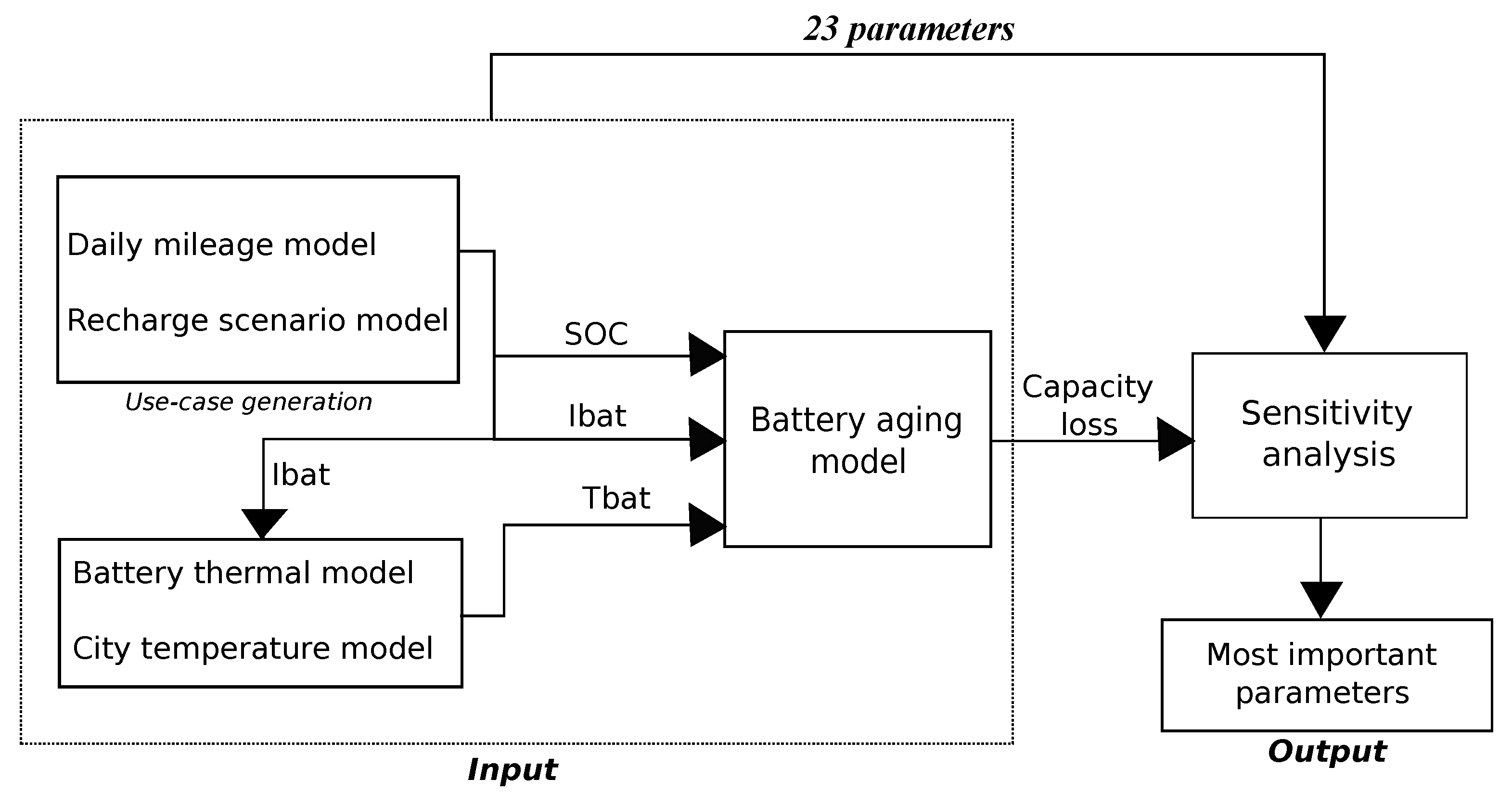
2. Methodological Approach

Figure 1 presents the flow chart of the model setup. Based on use case generation (daily mileage model, recharge scenario model, and battery size ($bat{t}_{size}$ parameter), the SOC is deduced. Then, the battery current $i_{batt}$ along one complete year at a step time of one minute is obtained. From the external or city temperature model and battery thermal model, the temperature of the battery is assessed along the year at the same sampling period, by calculating joule losses in the battery model using the variable battery current. From the SOC profile, battery current, and battery temperature, the aging model of the battery is used to assess the loss of capacity during one year of vehicle use. Using this complete aging model, a sensitivity analysis is performed (see Section 3). The following section presents in a detailed manner the different models used and developed for battery aging (see Section 2.1), uses case generation (see Section 2.2), and electrical and thermal model of the battery (see Section 2.3).

2.1. Battery Aging Model

Battery performance degrades over time due to battery aging. This performance degradation is caused by a loss of capacity and/or an impedance rise depending mainly on three factors: temperature, SOC, and current. Battery aging is classified into calendar aging and cycling aging. Calendar aging is the degradation during rest times (current, I = 0), whereas cycling aging is the degradation induced by charging and discharging the battery (I ≠ 0).

In this work, we used a combined multi-mechanism aging model based on Eyring laws, which was previously used and validated by [15,16,17]. The capacity loss rate $d{Q}_L/dt$ is divided into the calendar, cycling at cold temperature and hot temperature. The formula used is:

$$\frac{d{Q}_L}{dt}=\frac{d{Q}_{L,cal}}{dt}+\frac{d{Q}_{L,cyc,cold}}{dt}+\frac{d{Q}_{L,cyc,hot}}{dt}$$

(1)

with:

$$\frac{d{Q}_{L,cal}}{dt}=A_{cal}·e^{\left(\frac{-E_{a,cal}}{kT}+B_{cal}·SOC\right)}·f\left(Q_L\right)$$

(2)

$$\frac{d{Q}_{L,cyc,cold}}{dt}=A_c·e^{\left(\frac{-E_{a,c}+C_c·I}{k\left(T_o-T\right)}+B_c·SOC\right)}·f\left(Q_L\right)$$

(3)

$$\frac{d{Q}_{L,cyc,hot}}{dt}=A_h·e^{\left(\frac{-E_{a,h}+C_h·I}{kT}+B_h·SOC\right)}·f\left(Q_L\right)$$

(4)

$$f\left(Q_L\right)=\left(\frac{1}{1+b·Q_L^c}\right)$$

(5)

In each Eyring law from Equations (2) to (4), $A_i$ is the pre-exponential term in p.u.day${}^{-1}$, $E_{a,i}$ is the activation energy in eV, $B_i$ is the SOC influence parameter in p.u${}^{-1}$, and $C_i$ is the current influence parameter in hour.p.u${}^{-1}$ (with index i = cal, h, c for the calendar, hot cycling, and cold cycling, respectively). k is the Boltzmann constant in eV.K${}^{-1}$, T is the battery temperature in K, $T_o$ is the reference temperature in K, I is the current in A, and $Q_L$ is the capacity loss at time t in p.u. Equation (5) represents the dependence of $Q_L$ in $\frac{d{Q}_L}{dt}$. This equation induces a decrease in capacity loss rate as the battery ages, as it was found in preceding studies [18,19]. The values of all identified parameters (in Equations (2)–(5)) were calibrated to experimental results and data for different SOC and temperatures [15] to fit experimental results of calendar [16] and cycling aging tests [20]. Therefore, we assume here that this model is accurate enough to reproduce correctly the sensitivity to the studied parameters which is the main objective of our study. Hence, the parameters of the aging model itself are not considered in our sensitivity analysis. The only parameter considered for the battery aging model is the refreshing rate of capacity loss. To study the sensitivity analysis for the battery aging model, we vary the parameter $Q_{Lref}$, where capacity loss $Q_L$ refreshes as follows:

• $q{l}_{cst}$: $Q_L$ is assumed to be a constant;
• $q{l}_{min}$: $Q_L$ refreshes its value every minute;
• $q{l}_{day}$: $Q_L$ refreshes its value every day.

The model used comes from previous works in our laboratory and it was developed using many experimental data at different SOC and different temperatures. Therefore, we assume here that this model is accurate enough to reproduce correctly the sensitivity to the studied parameters which is the main objective of our study.

It must be noted that the refreshing of $Q_L$ need not match the time step to assess the aging (which is minutes in our study). This parameter can be important regarding the time of calculation because if it is greater than the step of time, it allows vectorizing the process which leads to a huge gain in computing efforts.

2.2. Use Cases Model Generation

The objective of the study is to analyze the impact of different parameters on battery aging, including annual mileage and place of residence. Parameterized use case scenarios are thus developed to generate driving and recharge scenarios. In our case, a German mobility survey [21] providing detailed information on travel patterns is used as the data source. A statistical approach based on logarithmic normal distribution is then applied to generate daily mileage. When some data are not available or when the accuracy is questionable, we try to parameterize the phenomenon to assess its sensitivity to battery aging.

2.2.1. Vehicle Uses

The statistical frequency of daily mileage is defined by a logarithmic normal distribution [22,23]:

$$D_m={\displaystyle \frac{1}{\sqrt{2\pi }\sigma D}}\exp {\displaystyle \frac{-{(\log D-\mu )}^2}{2{\sigma }^2}}·100$$

(6)

where D is the daily mileage in kilometers (km), $D_m$ is the occurrence of this mileage in %. $\mu$ and $\sigma$ represent the mean value and standard deviation of daily mileage log_norm distribution and depend on the annual mileage. They are interpolated using

Table 1. Mean value $\mu$ and standard deviation $\sigma$ of daily mileage log_norm distribution.

Annual Mileage	2500	7500	12,500	17,500	25,000	30,000
$\mu$	2.57	2.86	3.11	3.3	3.54	3.72
$\sigma$	1.05	1.05	1.06	1.03	1	1.18

and have been assessed using the least square method for German cases [24]. As the value of these two parameters, $\mu$ and $\sigma$, can change for other countries, the daily mileage generated will not be for Germany but can represent other countries that have other values for $\mu$ and $\sigma$. Hence, we applied two multiplier coefficients $coe{f}_{\sigma }$ and $coe{f}_{\mu }$ on $\sigma$ and $\mu$. These two coefficients are also parameters of our sensitivity analysis. Their effect can be seen in Figure 2, which shows the frequency of daily mileage for three sets of parameters $\mu$ and $\sigma$. The second and third sets are obtained by multiplying $\mu$ and $\sigma$, respectively, with 0.8 and 1.2.

Using Equation (6), the cumulative frequency distribution of daily driving distance can be assessed to generate classes of equal percentages. From each of these classes, the mean daily mileage can be calculated. Assuming a certain number of days per month $N_{travelmonth}$ when the vehicle is used (certain days may be off), the daily mileage for each of these $N_{travelmonth}$ is evaluated. The number of classes (equal to the number of days with trips) can be chosen differently for each month of the year. This is parameterized in our study by the parameter $mont{h}_{type}$ by considering all months to be identical or different months during the summer period.

Based on the daily mileage, information on the number of trips per day and speed will be necessary to assess the battery energy consumption (and fuel consumption). As it is difficult to have such information, the following assumptions are made linked to different parameters:

• Concerning the number of trips per day, it is assumed that under a certain daily mileage $D_{min}$, it corresponds to a short trip (for example, a shopping trip), with a quick return, and can thus be considered as a single trip;
• Above a certain daily mileage $D_{max}$, it is also considered as a single trip, for example, to go on holidays or long professional displacement;
• Between these two values, the daily mileage is separated into two trips assuming home-to-work and vice versa travel. In this case, the first travel takes place at $tim{e}_{ft}$ and the second at $tim{e}_{st}$.

The mean speed of this travel depends on the driving distance and Place of Residence ($PoR$). It is also assessed using statistical data coming from [24]. Figure 3 represents the mean speed of travel depending on its mileage for urban, extra-urban, and rural places of residence. The main difference between the places of residence appears for low to medium distances when the driving conditions differ. The mean speeds tend to equalize for long distances (>60 km), corresponding to highway conditions suggesting that driving style does not depend on the place of residence.

After acquiring the daily driving mileage and mean speed, the electric consumption (and fuel consumption) are assessed using three different driving cycles in urban, rural, and motorway conditions. From these cycles, the SOC variation (discharge) per kilometer can be calculated, which can then be used to obtain the SOC discharge profile. For the battery SOC management during the trip, we assume the following discharge strategy: the PHEV operates in an all-electric mode until a certain state of charge $So{C}_{sust}$. When this state of charge is reached the vehicle operates in charge-sustaining mode, and for battery aging consideration, the SOC is assumed to be constant in this mode.

The consumption of each driving cycle is calculated using VEHLIB Software [25] library. Each trip in a day is then described by a certain share of urban, rural, and motorway to respect the mean speed of the trip. The sharing on the driving cycle part is performed with the following rules:

• if ${\mathrm{V}}_{\mathrm{trip}}<{\mathrm{V}}_{\mathrm{urban}}$,
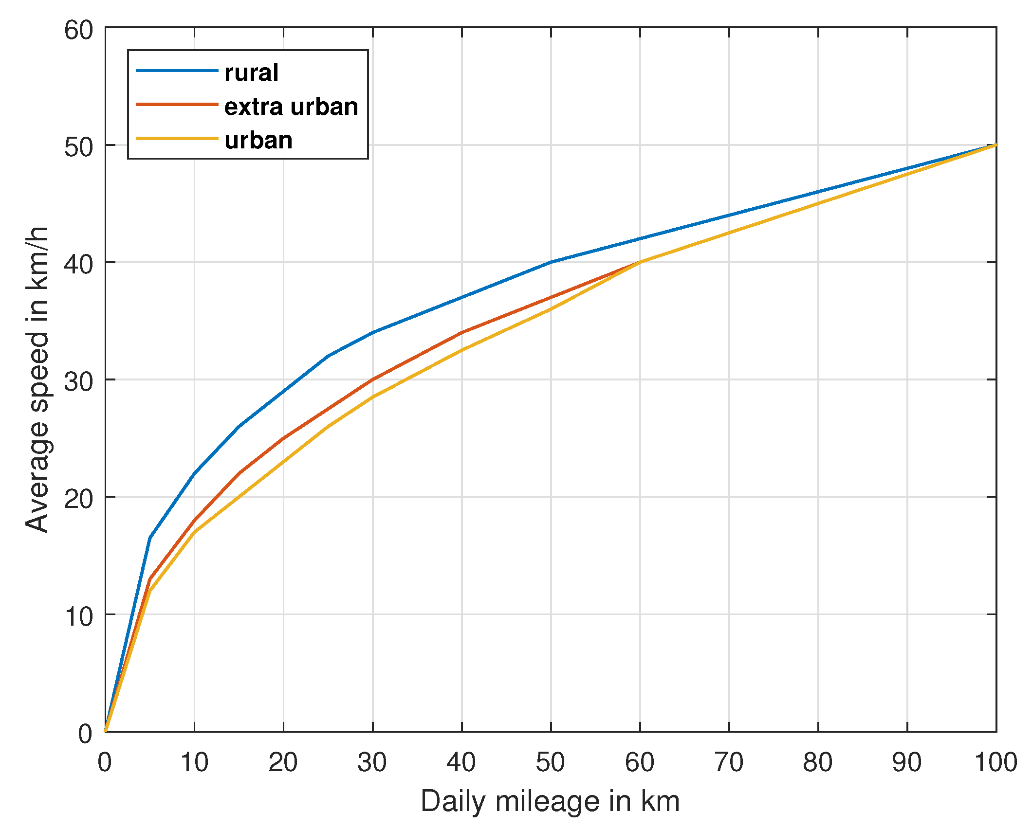
  all the travel is supposed to be urban.
• if ${\mathrm{V}}_{\mathrm{urban}}<{\mathrm{V}}_{\mathrm{trip}}<{\mathrm{V}}_{\mathrm{extra}}$,
  $urba{n}_{part}={\displaystyle \frac{{\mathrm{V}}_{\mathrm{extra}}-{\mathrm{V}}_{\mathrm{trip}}}{{\mathrm{V}}_{\mathrm{extra}}-{\mathrm{V}}_{\mathrm{urban}}}}$; $extr{a}_{part}=1-urba{n}_{part}$
• if ${\mathrm{V}}_{\mathrm{extra}}<{\mathrm{V}}_{\mathrm{trip}}<{\mathrm{V}}_{\mathrm{motorway}}$,
  $extr{a}_{part}={\displaystyle \frac{{\mathrm{V}}_{\mathrm{motorway}}-{\mathrm{V}}_{\mathrm{trip}}}{{\mathrm{V}}_{\mathrm{motorway}}-{\mathrm{V}}_{\mathrm{extra}}}}$; $motorwa{y}_{part}=1-extr{a}_{part}$
• if ${\mathrm{V}}_{\mathrm{trip}}>{\mathrm{V}}_{\mathrm{motorway}}$,
  all the travel is supposed to be on motorway,

where V represents the velocity in km/h.

To study the sensitivity of this sharing method and consumption assessment, different families of driving cycles are used:

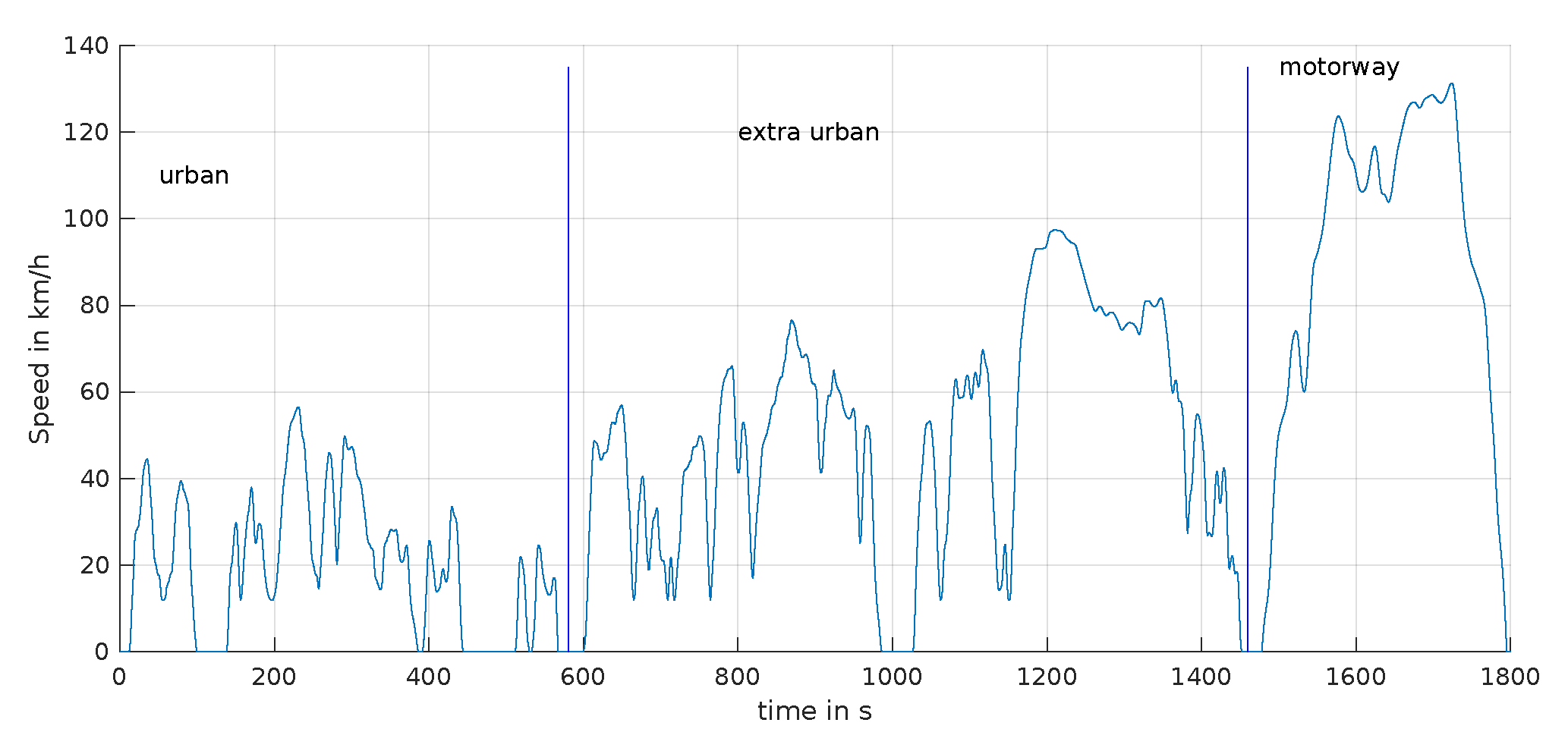
• One corresponds to the Worldwide harmonized Light-duty vehicles Test Cycles (WLTC) which is separated into three parts: urban, rural, and motorway, Figure 4;
• One is composed of the Artemis cycle which represents real driving conditions in urban, rural, and highway cases;
• One is composed of the Hyzem driving cycle [26] which has been specially developed to simulate and evaluate hybrid vehicles.

Table 2. Parameters of the sensitivity analysis.

Families	Parameters	Definition
Battery	$bat{t}_{size}$	battery size
Aging model	$Q_{Lref}$	capacity loss refreshment
Vehicle’s use	$km$	number of kms per year
	$PoR$	place of residence
	$N_{travelmonth}$	number of days with trips per month
	$tim{e}_{ft}$	time of first trip
	$tim{e}_{st}$	time of second trip
	$D_{min}$	max distance for short trip
	$D_{max}$	min distance for long trip
	$fa{m}_{cin}$	family of driving cycle
	$coe{f}_{\mu }$	mean value of daily mileage
	$coe{f}_{\sigma }$	standard deviation of daily mileage
	$So{C}_{sust}$	SOC sustaining threshold
	$mont{h}_{type}$	all months identical or not
Recharge scenarios	$c_{rate}$	charging rate
	$tim{e}_{rec}$	time of recharge
	$mo{d}_{rech}$	charging models
	$rec{h}_{soc-min}$	minimum SOC threshold
	$dis{t}_{pred}$	predict distance on the next day
Thermal model	$mo{d}_{therm}$	thermal model
	$city$	city of dwelling
	h	heat transfer coefficient
	$C_{th}$	specific thermal capacity

presents a summary of all the parameters taken into account in the sensitivity analysis arranged by the type of models (battery, aging model, vehicle’s use, recharge scenarios, and thermal model).

2.2.2. Recharge Scenario

These scenarios are created to study the effect of different charging times and strategies on the aging of the battery. Four different charging scenarios are created to define the parameter $mo{d}_{rech}$. A sensitivity analysis is also performed for these models with values of $mo{d}_{rech}$: $rec{h}_{trip}$, $rec{h}_{night}$, $rec{h}_{soc-trip}$, and $rec{h}_{soc-night}$.

In the $rec{h}_{trip}$ model, the battery is recharged after every single trip. Whereas, in the $rec{h}_{night}$ model, the battery is charged at a fixed time every night. In this study, the charging time is fixed by the parameter $tim{e}_{rec}$.

The other two models are based on the minimum SOC threshold. The first model in this case is $rec{h}_{soc-trip}$, in which the battery is recharged when the SOC passes below a minimum SOC threshold ($rec{h}_{soc-min}$), which can be possible either after the first or the second trip. The other model is $rec{h}_{soc-night}$, in which the battery is charged when the SOC is below the minimum threshold, but only at night.

We add a parameter to take into account a driver anticipating his next trip. If it is predicted that the distance to be covered in the next trip is greater than a certain value ($dis{t}_{pred}$), the battery is recharged before this trip using $rec{h}_{soc-trip}$ or at night using $rec{h}_{soc-night}$ models.

2.3. Electrical and Thermal Model of the Battery

We used an equivalent electrical circuit (OCV connected to an internal resistance) for the electrical battery model. The Equivalent electric Circuit Model (ECM) equation is presented below:

$$U_{bat}=OCV-R_{eq}·I_{bat}$$

(7)

where $I_{bat}$ is the battery current (positive when discharging) in A, $U_{bat}$ is the battery voltage in V, $OCV$ is the open circuit voltage in V, $R_{eq}$ is the internal resistance of the battery (in ohms) which has been calibrated with respect to a complex 2RC equivalent circuit model, by minimizing the difference in the output voltages of the two models (complex 2RC ECM and simple ECM) on a WLTC cycle.

The thermal model of the battery is based on a simple electro-thermal coupling equation as presented below:

$$C_{th}·\frac{d{T}_{bat}}{dt}=\frac{I_{bat}\left(U_{bat}-OCV\right)}{W_t}-\frac{h·A_{pack}\left(T_{bat}-T_{amb}\right)}{W_t}$$

(8)

Equation (7) in (8) gives:

$$C_{th}·\frac{d{T}_{bat}}{dt}=\frac{I_{bat}^2·R_{eq}}{W_t}-\frac{h·A_{pack}\left(T_{bat}-T_{amb}\right)}{W_t}$$

(9)

where $T_{bat}$ is the battery temperature in K, $T_{amb}$ is the ambient temperature in K, h is the heat transfer coefficient in W/(m${}^2·$K), $OCV$ is the open circuit voltage in V, $C_{th}$ is the specific thermal capacity of the battery in J/(Kg·K), $A_{pack}$ is the surface area of the battery pack in m², and $W_t$ is the weight of the battery pack in Kg. As the parameters h and $C_{th}$ are really difficult to assess precisely, they are also considered as parameters in our sensitivity analysis.

The ambient temperature is modeled using daily minimum ($T_{min}$) and maximum temperatures ($T_{max}$) varying throughout the year for different cities. The maximum temperature is assumed to occur at 5 p.m.

$$T_{amb}=\frac{T_{max}+T_{min}}{2}+cos(2·pi·\frac{t_{day}-17·24}{N_{md}})·\frac{T_{max}-T_{min}}{2}$$

(10)

where $N_{md}$ is the number of minutes in a day and $t_{day}$ is the time in minutes. To study the sensitivity of the variation of external temperature on battery aging, temperature models of three different cities—Abu Dhabi, Lyon, and Reykjavik—are created as examples for the analysis of temperature influence, to cover extremely hot, mean, and cold conditions, respectively. The data for daily minimum and maximum temperature come from [27] for the year 2021. The temperature profiles for Abu Dhabi, Lyon, and Reykjavik over a year are represented in Figure 5.

The thermal model of the battery as a parameter $mo{d}_{therm}$ is also studied with the sensitivity analysis of which the values differ as follows:

• $mo{d}_{therm}$ = $T_{amb}$; in this case, it is assumed that the battery temperature is equal to the external temperature;
• $mo{d}_{therm}$ = $mo{d}_{1D-Rcst}$; we use the thermal model of the battery but the resistance does not depend on the temperature but only on the SOC of the battery;
• $mo{d}_{therm}$ = $mo{d}_{1D-cpl}$; we use the thermal model of the battery, and the resistance depends on both the temperature and SOC of the battery.

The most accurate model is the one with resistance depending on the temperature. It leads to large computational time as the resistance has to be assessed at each step of the time.

Taking into account all the parameters involved in the above-defined models, a sensitivity analysis to identify the most influencing parameters is performed which is explained in the following section.

3. Model Integration and Sensitivity Analysis

Using the previously presented and developed models, a sensitivity analysis of battery aging for model-based PHEV use scenarios is performed. A SOC profile is obtained from daily mileage and recharge scenarios for one year. Figure 6 shows a typical SOC profile over a year on the left of the figure and zoom on the right for the month of January. This profile is obtained for one set of parameters and can be highly different for another set of parameters. For example, with higher annual mileage and other recharge parameters, the SOC can be below 50% for more than two days. A one-year profile was chosen to consider all the temperature variations during this period. From a sensitivity analysis point of view, this period seems relevant. It is difficult to reduce this period (except if the temperature has a low effect), but this duration can easily be increased in our model if we wish to consider thermal variation for a long-term and potential effect of previous capacity losses along the complete battery life. In the first approach, we considered that the battery aging is the same every year at least for its use in vehicles (capacity loss between 20 and 30%).

All the previously mentioned models have many different parameters which can influence the output, i.e., the capacity lost by the battery. For this reason, it becomes imperative to identify the most important input parameters which strongly influence the output. For that, a sensitivity analysis is performed.

In our study, we first chose 23 parameters (Table 2). In the first approach, each of these parameters can have between two and four values (generally three) chosen to represent extreme and mean values. This leads to a $8.4\times {10}^{10}$ set of parameters. It is then impossible to perform the simulation of the battery aging for all sets of parameters. For the first time, a “statistical approach” is performed to assess the conditional variance of each parameter and make the first discrimination of the most sensitive parameters. Then, as this approach can possess some statistical bias, a second analysis is performed on the most sensitive parameters with all the possible combinations.

In this statistical approach, the conditional variance is assessed for each parameter, using a sample of randomly chosen sets of parameters. For each parameter, $p_i$ of our study, a sample of 3000 sets of parameters is randomly selected by the Monte Carlo method. In the random sampling process, the parameter $p_i$ is not involved the first time. The sample is then triplicated for each value of the parameter $p_i$, leading to a sample of 9000 sets of parameters (if $p_i$ possesses three values).

This leads to a reasonable computing time of around 1 h per parameter in a computer with an Intel Xeon CPU—3.50 GHz with 2 processors, 8 cores, and 64GB RAM—by paralleling the processes. The complete sensitivity analysis is thus performed in around 1 day. The computing time to asses the battery aging for one set of a parameter depends on the parameter itself, especially on the thermal battery model $mo{d}_{therm}$ and on the capacity loss refreshment $Q_{Lref}$. It takes, on average, around 3 s for one assessment.

The conditional variance of the battery capacity losses is then assessed for each parameter $p_i$ :

$$var\left(Q_L\right|p_i)=\mathbb{E}\left({[Q_L-\mathbb{E}\left(Q_L\right|p_i)]}^2\right)\left|p_i\right)$$

(11)

where $Q_L$ is the loss of capacity, $p_i$ the $i^{th}$ parameter; $\mathbb{E}\left(X\right)$ is the mathematical expectation, i.e., the weighted average of X. $var\left(Q_L\right|p_i)$ represents the conditional expectation of $Q_L$, given $p_i$. It is then the expectation given $p_i$ of the square deviation between $Q_L$ and its conditional expectation given $p_i$. Assuming that we only focus on the simple “effect” of $p_i$ on $Q_L$ variance, and higher-order effect (for example, variance due to “coupling ” between two parameters) are neglected, $var\left(Q_L\right|p_i)$ is the part of the total variance of $Q_L$ explained by $p_i$. For the clarity of the result, it can be explained as the percentage of the total variance of $Q_L$ assessed by the sum of each conditional variance.

In the first approach, this conditional variance is only assessed on a sample of a randomly chosen set of parameters. In the second approach, to avoid statistical bias, the number of parameters is drastically reduced. The values of the non-sensitive parameter are fixed to a “mean” or “typical” value. The conditional variance of all parameters is assessed again with the same formula, but considering all the possible combinations of the selected parameters.

4. Results and Discussion

4.1. Use Cases

For the presented use cases, a Golf-GTE PHEV vehicle is modeled to assess the electric (and fuel) consumption along different driving cycles. The battery characteristics also correspond to this car. The main data are presented in

Table 3. PHEV—Golf GTE main characteristics.

Components	Characteristics	Values
Vehicle	weight	1480 kg
	aerodynamic coefficient $S·C_x$	0.0305 N·(m/s)${}^{-2}$
	rolling resistance $C_{rr}$	134 N
Battery	Capacity	24 Ah
	nominal voltage	345 V
	heat transfer coefficient	5 W/(m${}^2·$K)
	specific thermal capacity	900 J/(Kg·K)
	technology	Lithium ion
Engine	Max power	150 kW @ 5000–6000 rpm
	Max Torque	250 N.m @ 1600–3500 rpm
Electrical machine	Max power	75 kW
	Maximum torque	250 N.m
Auxiliary power	mean power	611 W

. The vehicle is simulated on VEHLIB Library ([25,28]), using the classical longitudinal forces model. The simulated consumption is validated with measurement on the WLTC cycle and shows less than 5% error. Currently, we do not use a thermal model of the cabin as performed in some studies [8,11,12]. The use of extra energy for air conditioning and heating is taken into account using a mean value. The auxiliary power is the sum of the power of “classical” accessories plus a mean value of the power required by air conditioning and heater. The value comes from an experimental campaign on a Golf-GTE instrumented in the city of Stuttgart [29].

Using the conditional variance approach, recall Section 3, a first study including all the parameters of our model is presented in

Table 4. Value of the parameter and sensitivity on battery aging.

Families	Parameters	Values	Sensitivity in%
Battery	$bat{t}_{size}$	12–24–36 Ah	32.4
Aging model	$Q_{Lref}$	minute–days	0.01
Vehicle’s use	$km$	7500–14,000–35,000 km	20
	$PoR$	urban–extra-urban–rural	0.08
	$N_{travelmonth}$	20–26–29	2.9
	$tim{e}_{ft}$	6–8–10 a.m.	0.03
	$tim{e}_{st}$	3–5–7 p.m.	0.004
	$D_{min}$	2–5–10 km	0.002
	$D_{max}$	80–100–200 km	0.8
	$fa{m}_{cin}$	WLTC–Artemis–Hyzem	0.8
	$coe{f}_{\mu }$	0.8–1–1.2	0.8
	$coe{f}_{\sigma }$	0.8–1–1.2	0.6
	$So{C}_{sust}$	30–40–50%	1.6
	$mont{h}_{type}$	ident–summer	0.02
Recharge scenarios	$c_{rate}$	$1/2$–$1/4$–$1/6$	0.8
	$tim{e}_{rec}$	9–10–11 p.m.	0.03
	$mo{d}_{rech}$	trip–night–soc_trip–soc_night	17.2
	$rec{h}_{soc-min}$	35–50–80%	1.12
	$dis{t}_{pred}$	0–50–100 km	0.01
Thermal model	$mo{d}_{therm}$	$t_{ext}$–$R_{cst}$–$R_{cpl}$	0.08
	$city$	Abu Dhabi–Lyon–Reykjavik	19.6
	h	2–5–8 W/(m${}^2·$K)	0.04
	$C_{th}$	500–900–1500 J/(Kg·K)	0.01

.

The discrete values used for each parameter correspond to typical minimum, maximum, and mean values:

• $bat{t}_{size}$: 24 Ah is the existing battery pack of Golf GTE, an electric range of 80 km, depending on the driving conditions, can then be expected. Three values of battery sizes were studied, corresponding to 0.5, 1, and 1.5 times the reference value (24 Ah) to match the minimum and maximum autonomy of existing PHEV cars.
• $Q_{Lref}$: Two values of capacity loss refreshing rate are included in this study: minute or day.
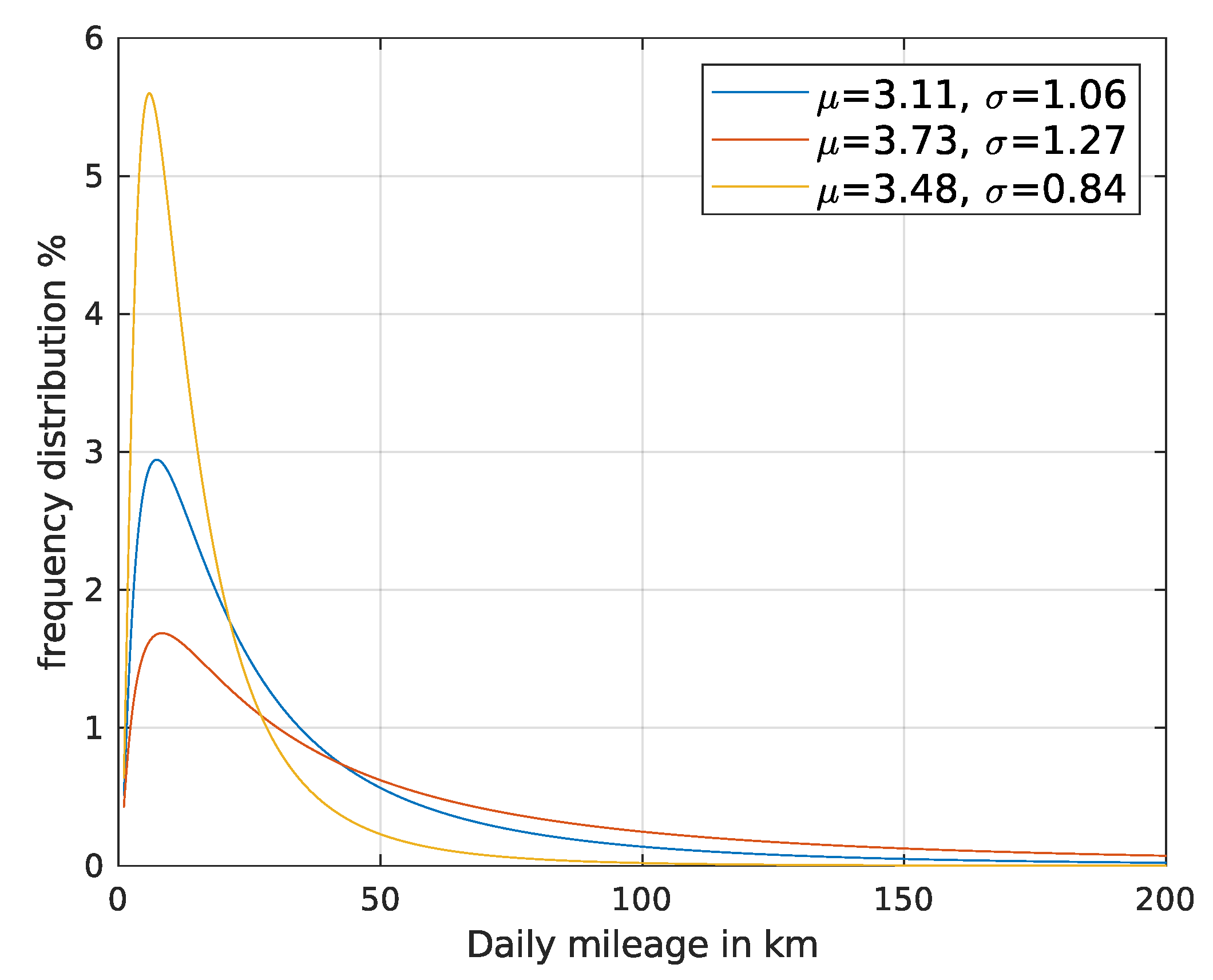
• km: The mean value of km per year, corresponding to the average annual mileage of German drivers [21].
• $c_{rate}$ value of $1/4$ is a classical value corresponding to a full battery recharge in 4 h.
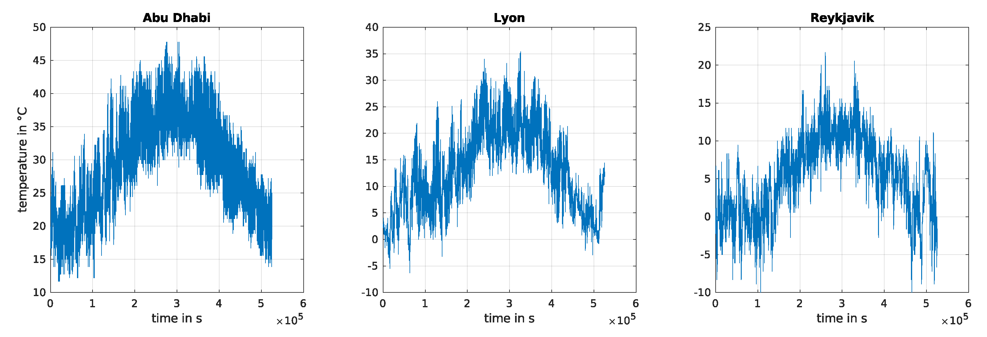
• $city$: Abu Dhabi and Reykjavik are chosen to represent extremely hot and cold climates, whereas Lyon represents average climatic conditions.
• h and $C_{th}$ have mean values corresponding to the experimental value determined in [7].
• $fa{m}_{cin}$: WLTC, Artemis, and Hyzem driving cycles are studied.
• $mont{h}_{type}$: Two cases are studied, one where the daily mileage is the same for each month of the year, this seems reasonable regarding [21]. A case with different driving behavior in summer, trying to consider holiday trips, was added.
• $So{C}_{sust}$: In the Golf GTE (and other PHEVs), the SOC strategies often discharge the batteries to a low SOC threshold and then operate the vehicle in charge-sustaining mode. From an energetic point of view, and aiming to transfer a maximum of fuel consumption to electricity, the minimum SOC threshold has to be as low as allowable by the battery. We nevertheless study two cases at 40 and 50% to assess their effect on battery aging.

For other parameters, the values are chosen to be coherent with our model (for example, time of the first travel has to remain before the time of the second travel, $D_{min}$ has to remain inferior to $D_{max}$). The aim is often to verify that these parameters do not affect aging.

4.2. Results

The main sensitive parameters (Table 4) in decreasing order are: the battery size $bat{t}_{size}$, the number of kilometers per year km, the external temperature represented by a city $city$, the recharge strategy $mo{d}_{rech}$, and on a second order, the number of trips per month $N_{travelmonth}$, SOC sustaining threshold $So{C}_{sust}$, and the minimum SOC when recharging below a threshold $rec{h}_{soc-min}$. Other parameters have no impact on the battery aging (less than 1%). This sensitivity is discussed in Section 4.3.

To avoid statistical bias, a second analysis is performed, only on these seven parameters assessing all the set of variables. The conditional variances are presented in

Table 5. Sensitivity value for selected parameters.

Families	Parameters	Values	Sensitivity in%
battery	$bat{t}_{size}$	12–24–36 Ah	36.3
Vehicle’s use	$km$	7500–14,000–35,000 km	15.8
	$N_{travelmonth}$	20–26–29	3.9
	$So{C}_{sust}$	30–40–50%	1.7
Recharge scenarios	$mo{d}_{rech}$	tra–night–$so{c}_{tra}$–$so{c}_{night}$	20.3
	$rec{h}_{soc-min}$	35–50–80%	1.4
Thermal model	$city$	Abu Dhabi–Lyon–Reykjavik	20.6

. The values of these seven parameters are the same as in the first analysis. For the sixteen other parameters, mean values are retained. This leads to 2916 assessments of our model and represents less than 1 h of computational time. The sensitivity results are presented in Table 5. These results have close values compared to the results from the first analysis, proving that a sample of 3000 sets of parameters does not quite have a statistical bias.

In this analysis, the aging varies from a minimum value of 1.16% loss of capacity to a maximum loss of 5.36% in one year. The mean loss value is 2.65%. The parameters for min and max losses of capacity are presented in

Table 6. Value of parameters for min and max capacity loss.

${\mathit{Q}}_{\mathit{L}}$	${\mathit{batt}}_{\mathit{size}}$	$\mathit{km}$	${\mathit{N}}_{\mathit{travelmonth}}$	${\mathit{SoC}}_{\mathit{sust}}$	${\mathit{mod}}_{\mathit{rech}}$	${\mathit{rech}}_{\mathit{soc}-\mathit{min}}$	$\mathit{city}$
1.16%	36 Ah	7500 km	20	30%	soc_night	35%	Reykjavik
5.36%	12Ah	35,000 km	29	30%	tra	35%	Abu Dhabi

. On the one hand, the minimum aging occurs in cold conditions (Reykjavik) for the large-sized battery, recharging only at night if the SOC is below 35% and for minimum travel per month. On the other hand, the maximum aging occurs in hot conditions (Abu Dhabi), for a small-sized battery, recharging after each travel and traveling 29 days per month. In the two cases, the SOC sustaining threshold is 30%.

4.3. Discussion

The two previous analyses (Table 4 and Table 5) provide important information on the sensitivity of different parameters on the battery aging of PHEV considering model-based use case scenario generation. As a first goal of this study, many parameters of our models can be neglected in future studies as they have no impact on battery aging. In future studies, for example, focusing on environmental impacts or battery sizing, a mean value can then be adapted. This is the case for:

• The aging refreshment, which can be fixed to one day (refreshing $Q_L$ each day) and thus reduces the computational effort;
• The place of residence, at least in the manner we modeled it, i.e., a modification of the mean speed of travel (see Section 2.2);
• The family of driving cycles does not quite have an effect as this only changes the rate of discharge of the battery and does not drastically affect the SOC profile. For battery aging, it has no effect but can be sensitive in LCA as it will change the electrical (and thus fuel) consumption;
• The parameters linked to daily mileage generation ($coe{f}_{\mu }$, $coe{f}_{\sigma }$, $mont{h}_{type}$,) and the sharing between one or two trips ($D_{min}$, $D_{max}$). This tends to prove that a daily mileage statistical approach is accurate enough for battery aging consideration;
• The parameters to assess the SOC profile that depends on the time of travel ($tim{e}_{ft},tim{e}_{st}$);
• The thermal model parameters ($mo{d}_{therm}$), and thus the thermal model, do not quite have an impact. It was found in the first complete sensitivity analysis that this parameter has an impact of 0.08% which means that using either a simple model or an accurate one has no effect on the battery aging in our case. Therefore, we use a simple model to reduce the computational burden and in our case, the battery temperature can be considered to be equal to the external temperature. This can be explained by the fact that in our scenarios, the car is used for a really small part of the time (less than 5% of the time for 14,000 km annual mileage). Thus, the temperatures are relatively identical whether we consider the thermal model or not. This conclusion will not be acceptable for other uses of vehicles—public transport, vehicle sharing—where the battery usage affect its internal temperature (Joules losses);
• The battery recharge rate $c_{rate}$ has no effect, or second-order effect, probably because the SOC profiles are not very affected by this parameter. However, fast recharge has not been considered here and the conclusion is only valid for slow recharge;
• The time of recharge $tim{e}_{rec}$ (in case of night recharge) is also non-sensitive (or its variation is too small);
• The predictive distance parameter ($dis{t}_{prev}$) does not quite have an effect either as it does not change the global SOC profile (it acts only on a few days per year for our scenario).

If some parameters used to generate the recharge scenario do not quite have an effect, some parameters are highly sensitive to battery aging. The recharge scenario ($mo{d}_{rech}$), is one of them. This can be explained by the fact that it highly changes the SOC profile, especially if the battery is recharged only when the SOC reaches a certain threshold ($mo{d}_{rech}=so{c}_{trip}$ or $so{c}_{night}$). Depending on the daily mileage, the battery can be recharged only after a couple of days instead of after each travel or each day, thus, the SOC remains possibly relatively small for several days.

The manner of generating the charging scenarios is thus really sensitive and has to be further investigated. The order of travel linked to the variability of daily mileage (which cannot be considered constant) can surely influence the results (succession of days with small or no travel, for example). Special attention thus has to be paid to future studies on these parameters. It is also possible to complete this study by adding other parameters to generate other scenarios and show the most sensitive parameters and phenomena.

The external temperature also has an important influence on our model even if the battery thermal model itself is not sensitive. This point could also be further investigated using a more precise model of air-conditioning and heating (cabin thermal model for instance). The auxiliary power can then fluctuate with time and will depend on the external temperature. This can affect the SOC and thus the aging. The external temperature, which is already a sensitive parameter, may then be more important.

The other sensitive parameters are battery size ($bat{t}_{size}$), the annual mileage ($km$), and the SOC sustaining threshold ($So{C}_{sust}$), all of which have a high influence on the battery SOC profile and thus on the aging. The number of travels per month $N_{travelmonth}$ have a second-order influence (around ten times less than other parameters).

5. Conclusions

A sensitivity analysis on the battery aging of a PHEV was performed. It is based on parameters allowing the generation of statistical model-based PHEV use case scenarios and using a pre-validated battery aging model.

It shows that the most important parameters to be considered for battery aging are: battery size, external temperature, annual mileage, and the parameters describing recharge scenarios. The driving cycle’s use for electric and fuel consumption assessment and battery thermal model seems to have a small effect on battery aging for personal car usage. The number of parameters to be considered in the battery aging study has thus been drastically reduced and the sensitivity analysis proves that some parameters will have close to no effect on the battery aging (slow charging rate, place of residence, etc.)

However, further investigation has to be performed considering battery recharge scenarios and their link to daily mileage variability generation. The non-sensitivity of the battery thermal model is also questionable for the case of vehicles that are in use for a large part of the time. As the generation of scenarios is based on statistical data, the vehicles’ use is representative of the mean behavior of drivers traveling a certain mileage per year. The sensitivity and the battery aging could then be different in some specific cases where the driving behavior is very different from the ones noted in the statistical data.

This study provides important leads on the parameters to be considered in future work on complete LCA assessment including battery aging and optimal sizing of PHEV.

References

- European Commission. CO2 Emission Performance Standards for Cars and Vans; European Commission: Brussels, Belgium, 2021. [Google Scholar]
- Smith, K.; Warleywine, M.; Wood, E.; Neubauer, J.; Pesaran, A. Comparison of Plug-in Hybrid Electric Vehicle Battery Life across Geographies and Drive-Cycles; SAE Technical Papers; SAE International: Warrendale, PA, USA, 2012. [Google Scholar] [CrossRef]
- Yuksel, T.; Litster, S.; Viswanathan, V.; Michalek, J.J. Plug-in hybrid electric vehicle LiFePO4 battery life implications of thermal management, driving conditions, and regional climate. J. Power Sources 2017, 338, 49–64. [Google Scholar] [CrossRef]
- Onori, S.; Spagnol, P.; Marano, V.; Guezennec, Y.; Rizzoni, G. A new life estimation method for lithium-ion batteries in plug-in hybrid electric vehicles applications. Int. J. Power Electron. 2012, 4, 302–319. [Google Scholar] [CrossRef]
- Plötz, P.; Moll, C.; Bieker, G.; Mock, P.; Li, Y. Real-World Usage of Plug-in Hybrid Electric Vehicles: Fuel Consumption, Electric Driving, and CO2 Emissions; Technical report; The Intenational Council on Clean Transportation (ICCT): Berlin, Germany, 2020. [Google Scholar]
- Lunz, B.; Yan, Z.; Gerschler, J.B.; Sauer, D.U. Influence of plug-in hybrid electric vehicle charging strategies on charging and battery degradation costs. Energy Policy 2012, 46, 511–519. [Google Scholar] [CrossRef]
- Houbbadi, A.; Redondo-Iglesias, E.; Trigui, R.; Pelissier, S.; Bouton, T. Optimal Charging Strategy to Minimize Electricity Cost and Prolong Battery Life of Electric Bus Fleet. In Proceedings of the 2019 IEEE Vehicle Power and Propulsion Conference (VPPC), Hanoi, Vietnam, 14–17 October 2019; pp. 1–6. [Google Scholar] [CrossRef]
- Tang, L.; Rizzoni, G.; Cordoba-Arenas, A. Battery Life Extending Charging Strategy for Plug-in Hybrid Electric Vehicles and Battery Electric Vehicles. IFAC-PapersOnLine 2016, 49, 70–76. [Google Scholar] [CrossRef]
- Su, W.; Chow, M.Y. Sensitivity analysis on battery modeling to large-scale PHEV/PEV charging algorithms. In Proceedings of the IECON 2011—37th Annual Conference of the IEEE Industrial Electronics Society, Melbourne, VIC, Australia, 7–10 November 2011; IEEE: New York, NY, USA, 2011; pp. 3248–3253. [Google Scholar]
- Zhang, S.; Hu, X.; Xie, S.; Song, Z.; Hu, L.; Hou, C. Adaptively coordinated optimization of battery aging and energy management in plug-in hybrid electric buses. Appl. Energy 2019, 256, 113891. [Google Scholar] [CrossRef]
- Sockeel, N.; Shi, J.; Shahverdi, M.; Mazzola, M. Sensitivity analysis of the battery model for model predictive control: Implementable to a plug-in hybrid electric vehicle. World Electr. Veh. J. 2018, 9, 45. [Google Scholar] [CrossRef]
- López-Ibarra, J.A.; Goitia-Zabaleta, N.; Herrera, V.I.; Gazta, H.; Camblong, H. Battery aging conscious intelligent energy management strategy and sensitivity analysis of the critical factors for plug-in hybrid electric buses. ETransportation 2020, 5, 100061. [Google Scholar] [CrossRef]
- Xie, S.; Hu, X.; Qi, S.; Tang, X.; Lang, K.; Xin, Z.; Brighton, J. Model predictive energy management for plug-in hybrid electric vehicles considering optimal battery depth of discharge. Energy 2019, 173, 667–678. [Google Scholar] [CrossRef]
- Yang, L.; Sandeep, M. PHEV Hybrid Vehicle System Efficiency and Battery Aging Optimization Using A-ECMS Based Algorithms; Technical report, SAE Technical Paper 2020-01-1178; SAE International: Warrendale, PA, USA, 2020. [Google Scholar] [CrossRef]
- Houbbadi, A.; Redondo-Iglesias, E.; Pelissier, S.; Trigui, R.; Bouton, T. Smart charging of electric bus fleet minimizing battery degradation at extreme temperature conditions. In Proceedings of the 2021 IEEE Vehicle Power and Propulsion Conference (VPPC), Gijon, Spain, 25–28 October 2021; pp. 1–6. [Google Scholar] [CrossRef]
- Redondo-Iglesias, E.; Venet, P.; Pelissier, S. Eyring acceleration model for predicting calendar ageing of lithium-ion batteries. J. Energy Storage 2017, 13, 176–183. [Google Scholar] [CrossRef]
- Redondo-Iglesias, E.; Vinot, E.; Venet, P.; Pelissier, S. Electric vehicle range and battery lifetime: A trade-off. In Proceedings of the EVS32; 32nd Electric Vehicle Symposium (EVS32), Lyon, France, 19–22 May 2019; p. 9. [Google Scholar]
- Broussely, M.; Herreyre, S.; Biensan, P.; Kasztejna, P.; Nechev, K.; Staniewicz, R. Aging mechanism in Li ion cells and calendar life predictions. J. Power Sources 2001, 97–98, 13–21. [Google Scholar] [CrossRef]
- Spotnitz, R. Simulation of capacity fade in lithium-ion batteries. J. Power Sources 2003, 113, 72–80. [Google Scholar] [CrossRef]
- Song, Z.; Li, J.; Han, X.; Xu, L.; Lu, L.; Ouyang, M.; Hofmann, H. Multi-objective optimization of a semi-active battery/supercapacitor energy storage system for electric vehicles. Appl. Energy 2014, 135, 212–224. [Google Scholar] [CrossRef]
- Claudia, N.; Kuhnimhof, T. Mobilität in Deutschland—MiD Ergebnisbericht; Technical report, Studie von infas, DLR, IVT und infas 360 im Auftrag des Bundesministers für Verkehr und digitale Infrastruktur (FE-Nr. 70.904/15); Institute of Transport Research: Berlin, Germany, 2018. [Google Scholar]
- Redelbach, M.; Özdemir, E.D.; Friedrich, H.E. Optimizing battery sizes of plug-in hybrid and extended range electric vehicles for different user types. Energy Policy 2014, 73, 158–168. [Google Scholar] [CrossRef]
- Bleymüller, J.; Weißbach, R.; Dörre, A. Statistik für Wirtschaftswissenschaftler; Vahlen: Munich-Schwabing, Germany, 2020. [Google Scholar]
- Nirk, T. The Influence of Use Cases on Life Cycle Assessement Result of Plug in Hybrid Vehicle. Master’s Thesis, Faculty for Technology, Hochschule Pforzheim, Pforzheim, Germany, 2019. [Google Scholar]
- Vinot, E.; Scordia, J.; Trigui, R.; Jeanneret, B.; Badin, F. Model simulation, validation and case study of the 2004 THS of Toyota Prius. Int. J. Veh. Syst. Model. Test. 2008, 3, 139–167. [Google Scholar] [CrossRef]
- Barlow, T.J.; Latham, S.; McCrae, I.S.; Boulter, P.G. A reference book of driving cycles for use in the measurement of road vehicle emissions; Technical report; TRL Limited: Berkshire, UK, 2009. [Google Scholar]
- Meteociel. Available online: https://www.meteociel.fr/climatologie/obs_villes.php (accessed on 10 March 2022).
- Jeanneret, B.; Redondo-Iglesias, E.; Trigui, R.; Vinot, E. Vehlib. Available online: https://gitlab.univ-eiffel.fr/eco7/vehlib (accessed on 10 March 2022).
- Ehrenberger, S.; Philipps, F.; Konrad, M. Analysis of Pollutant Emissions of Three Plug-in Hybrid Electric Vehicles; Transport and Air Pollution (TAP): Thessaloniki, Greece, 2019. [Google Scholar]