Article

Evaluation of the Effects of Coal Jigging by Means of Kruskal–Wallis and Friedman Tests

by
Tomasz Niedoba
1,*,
Agnieszka Surowiak
1,
Ahmad Hassanzadeh
2,3 and
Hamid Khoshdast
4,5
1
Department of Environmental Engineering, Faculty of Civil Engineering and Resources Management, AGH University of Science and Technology, al. Mickiewicza 30, 30-059 Krakow, Poland
2
Department of Geoscience and Petroleum, Faculty of Engineering, Norwegian University of Science and Technology, 7491 Trondheim, Norway
3
Maelgwyn Mineral Services Ltd., Ty Maelgwyn, 1A Gower Road, Cathays, Cardiff CF24 4PA, UK
4
Department of Mining Engineering, Higher Education Complex of Zarand, Zarand 77611-56391, Iran
5
Mineral Industries Research Center, Shahid Bahonar University of Kerman, Kerman 76169-13439, Iran
*
Author to whom correspondence should be addressed.
Energies 2023, 16(4), 1600; https://doi.org/10.3390/en16041600
Submission received: 9 January 2023 / Revised: 30 January 2023 / Accepted: 1 February 2023 / Published: 5 February 2023
(This article belongs to the Special Issue Factor Analysis and Mathematical Modeling of Coals)

Abstract

:
Coal beneficiation processes are often based on gravitational enrichment techniques. Therefore, various types of jigs are often used in this area. A number of factors determine the quality of the final product. Therefore, proper and systematic monitoring of such a process is necessary. The present work examined the effect of the hutch water amount and the amount of processed coal (system capacity) on the yield and ash grade in individual density–size fractions. A statistical method in the form of the Kruskal–Wallis test and the Friedman test was used to evaluate the process. These tests were proposed as universal and reliable alternatives to classical analysis of variance (ANOVA) analysis. The performed analysis allowed for the determination of what process conditions should be selected in order to obtain certain effects. Therefore, it allowed us to apply certain combinations of hutch water amount, system capacity and particle characteristics to maximize the expected effects. The application of statistical analysis methods in the form of Kruskal–Wallis and Friedman tests to evaluate process efficiency creates new possibilities to monitor and optimize the jigging process in both context of amount and quality of final product and is very important not only for mining enterprise but also from an environmental point of view.

1. Introduction

Quantitative and qualitative characteristics of the basic coal components and their physicochemical properties are important elements in the selection of optimal methods for processing purposes. At the same time, in the era of the development of modern and highly efficient combustion technologies of solid fuel and the deterioration in the quality of deposits, it is necessary to thoroughly analyze the properties of coal particle size fractions, especially fine ranges, which are predominant ones in the market.
In the case of coal, these features consist of ash grade, sulfur grade, combustion heat, volatile component grade and analytic moisture. The features mentioned above determine coal quality and as a result, its economic value. Because of this, the utmost care has to be taken in determining coal quality.
The knowledge about the features describing coal quality can also serve for evaluating beneficiation processes [1,2,3,4,5,6,7,8]. The ash grade, sulfur grade and volatile parts grade were examined depending on particle size and particle density, also by means of the kriging method [4] or non-parametric statistical methods [9].
A typical factor analysis was conducted by Niedoba et al. recently [10]. Multidimensional methods can also be used to assess the effectiveness of beneficiation processes. In this regard, the following methods were applied for a number of research works: observational tunnels method [11], principal component analysis [12,13], relevance maps [14], self-organizing Kohonen maps [15], multidimensional scaling [16] and autoassociative neural networks [17]. A comparison of these methods and their effectiveness was presented in detail elsewhere [18].
To control the quality of a beneficiation process and the raw material itself, it is necessary to properly monitor and systematically adjust the coal quality parameters. This can be executed according to various criteria adopted by the analyst. Such criteria can be the yield of a useful component [19], the type of device, and/or the principal goal of the process. Many studies have dealt with various approaches to this end. Radiometric density measurements have been used to model the process in many studies [20,21,22]. Numerical studies in multiphase flow have been presented in several research works [23,24]. For instance, the jig frequency was examined by Tripathy et al. [25]. Classical statistical methods were used in this respect [26], as well as “black box” methods based on neural networks [27]. The application of coupled fuzzy logic and experimental design can be found in [28]. Modeling of the influence of mechanical parameters of the device on the hydrodynamic behavior has been presented in [29]. More advanced approaches using 3D response methodology [30] or computational fluid dynamic (CFD) simulations [31,32] have also been employed successfully. Modeling with the use of “artificial intelligence” has also performed [33]. In addition, many different types of jigs have been tested for the efficiency of the beneficiation process. Dry jigging has been discussed in many papers [34,35,36]. The use of the altair jig has been presented in another investigation [37]. In turn, the Kelsey jig has been reported by Richards et al. [38]. Another approach was fluid motion modeling, adopted in other works [39,40], or the testing of the shape of the material particles [41,42]. Other than these, the trends and potential development of jig applications in the processing industry have been discussed elsewhere [43,44,45,46].
The pulsation cycle involving the amount of so-called hutch water is an important hydrodynamic factor affecting the beneficiation process in the jig. Its influence on the process itself has been discussed in-depth previously [8,47,48,49,50,51,52,53]. The pulsating motion of the water should be selected to ensure that the particles settle as the water is directed down the unit. The pulsation cycle can be symmetrical or asymmetrical. In the first case, the times of rising and falling particles are the same, while in the second treatment, these times are different. Thus, the pulsation characteristics of the water greatly influence the achievement of the best possible results of the beneficiation process. This in turn is affected by the appropriate amount and time of air supply as well as the frequency of pulsation [54].
As the material is directed down the device, some of the fine particles are somehow “trapped” by the coarser ones and thus are also directed to the settling product. This obviously affects the efficiency of the process. Therefore, hutch water is included in the feed process, which allows the fine particles to be carried back to the overhead product. Thus, hutch water helps to reduce the negative impact of the phenomenon discussed above. The amount of water is also important so that it can effectively influence the “release” of fine particles from the falling product. This phenomenon has been discussed and presented separately in work performed by Blaschke [55]. The present study analyzes the effects of coal beneficiation in a jig. The aim of the article is to demonstrate the effect of the amount of hutch water and the processed coal on the yield and ash grade in individual density–size fractions of the obtained coal concentrates. In order to achieve the set aim of this work, in the first stage, an experiment was carried out by testing an industrial jig and changing the technological and hydrodynamic operating conditions. The second stage of the experiments involved the laboratory analysis of the beneficiation products in terms of the quantity and quality of separated concentrates in narrow density–size fractions. The results were evaluated using the Kruskal–Wallis and the Friedman tests, which can be used universally, regardless of the type of distribution of random variables. Thus, they can be presented as alternatives to traditional ANOVA analysis, which is not always possible due to not meeting certain conditions, which are mainly [56,57]:
-
Each population has to represent a normal distribution;
-
The samples must be independent;
-
Samples collected from each population must be random and simple;
-
Variances in populations must be equal.
This methodology has been used in many fields of science and is still under development. It has been applied in many scientific works, not only in mathematics and statistics [58,59]. It has also been directly combined with classical ANOVA [60,61,62], as well as the Monte Carlo method [63]. It has also been used in image analysis [64], but more frequently in medical as well as educational and sociological analyses [65,66]. In particular, it has also been applied to the analysis of data concerning the COVID-19 pandemic [67]. Therefore, it can be efficiently considered in several areas. In this work, the presented approach was applied to evaluate the influence of hutch water amount and system capacity during jigging on selected coal parameters (yield and ash grade). Through this, it was possible to optimize the process conditions for the given responses. The analysis of the results of industrial jig work presented in a statistical way with the application of not-common methods can be used as a way to expand the knowledge of the analysis and the description of beneficiation processes.

2. Materials and Methods

2.1. Experiments

The experiments of coal beneficiation and analyses of jig work were conducted in two stages. The first one was based on the sampling of an industrial jig and the second one was performed through chemical laboratory research works. The sampling of industrial jig was implemented in one of the mechanical coal processing plants located in Poland in which coals of particle size < 20 mm were enriched. This was the matter for the steam coal, type 31.1, according to Polish classification. The cycle of performed experiments was based on the sampling of separation products, i.e., concentrate, middlings and tailings (every 3 min, one sample was taken for each stream). This was undertaken after stabilization of the process, meaning after obtaining certain feed stream flows and amount of added hutch water. Under such a condition, 120 kg of the material in total was sampled from one experiment, so by one position of capacity and amount of hutch water. The working surface of the bed was equal to 17 m2, with an amplitude of 110 mm.
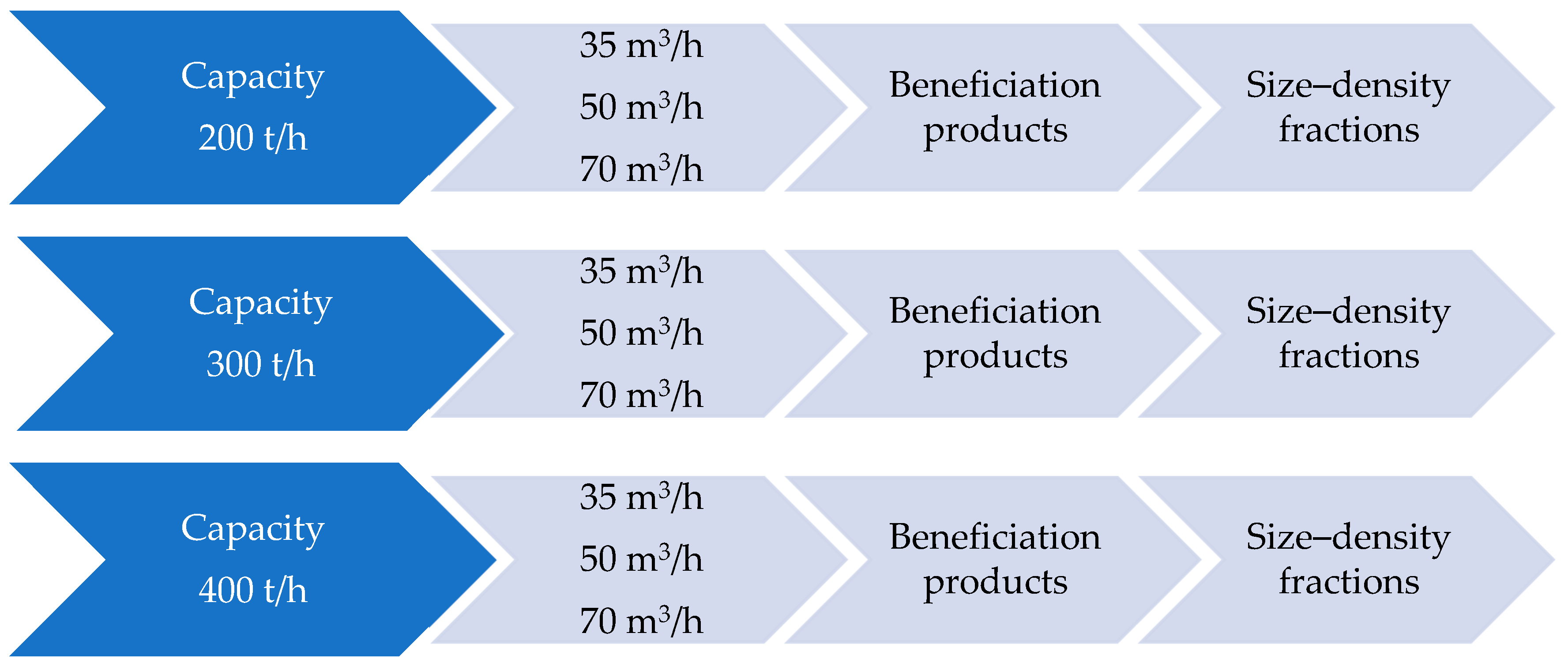
The experiments were carried out while maintaining a constant number of pulsations of the working bed, which was 26 cycles per minute. A total of 9 experiments were carried out, with the capacity and the amount of hutch water being changed in the jig each time. The capacity of the system, i.e., the flow rate of the feed in the experiments, was 200, 300 and 400 t/h, respectively, and the settings for the amount of hutch water for the set jig capacities were 35, 50 and 70 m3/h. Industrial experiments were performed at the set operation parameters and representative samples were obtained for further analyses. Then, each of the separation products was subjected to laboratory float–sink and size analyses. The float–sink analysis was performed in zinc chloride solutions with densities of 1.3, 1.4, 1.5, 1.6, 1.7, 1.8 and 2.0 t/m3. The separated density fractions of all samples were screened using sieves with the mesh sizes of 2.0, 3.15, 5.0, 6.3, 8.0, 10.0, 12.5, 16.0 and 20.0 mm. As a result, size–density fractions were obtained and classified according to the particle size and density of the material simultaneously.
In all size–density fractions obtained through float–sink and size analysis, mass yields of products and ash grade were determined. The size–density fractions of concentrates obtained from all industrial experiments were subjected to a detailed statistical analysis.
The industrial experiment was carried out with the following jig settings:
  • v—system capacity: 200, 300 and 400 t/h;
  • u—amount of hutch water: 35, 50 and 70 m3/h.
The model of the factorial experiment is presented in Figure 1.

2.2. Methodology

Mathematical analysis of the results was performed for the obtained size–density fractions of concentrates from each experiment in order to determine the influence of process parameters, i.e., yield and hydrodynamic parameters and the amount of hutch water on beneficiation of commercial products. Therefore, for each particle size fraction, the following formula was considered:
Ψ ( y i , u , v ) = ( x i 1 , x i 2 , , x i 8 )
where:
Ψ—the mapping which assigns to each middle of particle size fraction, yi, by a certain amount of hatch water, u, and system capacity, v, a vector which coordinates mean yield of the material originating from i-th particle size fraction in individual particle density fraction;
  • yi—center of i-th particle size fraction (according to particle size);
  • xij—share percentage of yield in i-th particle size fraction and j-th density fraction;
  • u—amount of hutch water (u∈{35, 50, 70});
  • v—capacity (v∈{200, 300, 400});
  • i = 1, 2,…, 9; j = 1, 2,…, 8.
The Kruskal–Wallis and the Friedman tests were used to examine the dependence of the yield distribution in a given particle size fraction on the amount of used hutch water and system capacity. The conditions to perform ANOVA analysis were not fulfilled (normality of distributions, and equality of variances).
The Kruskal–Wallis test is the non-parametric equivalent of the one-way ANOVA. It can be used when the goal is to compare three or more groups on some quantitative variable. Compared to classical ANOVA, however, there are several fundamental differences. It is a non-parametric test, meaning it can be utilized when assumptions about parametric tests are not met. This makes it a universal tool. The Kruskal–Wallis test compares each observation against the median, which means that it compares sums of ranks, not means or variances. Therefore, when reporting its results, it is worth paying attention to the value of the median in all groups and drawing conclusions on this basis, and not by comparing the means [68,69,70].
Another non-parametric test used to compare means in several dependent groups was the Friedman test. It is typically applied when the variables do not meet the assumptions of the analysis of variance in a repeated measures design. Its calculation scheme is based on ranking measurements, i.e., assigning weights to them in ascending order. The method uses an approximation applying the χ2 distribution [71].
First, the dependencies of the yield distribution in individual particle size fractions were examined at a fixed value of the variable u (i.e., the amount of hutch water) for successive values of the variable v (system capacity) and then the same calculations were repeated by setting the values of the variable v and changing the values of the variable u. They were denoted by Fij(x) distribution functions of random variables, which assumed the values of the output volume (in %) in a given density fraction at fixed values of u and v, where i = 1, 2, 3; and j = 1, 2, 3. The H0 hypothesis was checked, represented by
H 0 : F i 1 ( x ) = F i 2 ( x ) = F i 3 ( x ) ,   i = 1 ,   2 ,   3
against the hypothesis H1 that these distributions are not equal.
The Kruskal–Wallis test was used according to Equation (3):
H = 12 n ( n + 1 ) i = 1 k R i 2 n i 3 ( n + 1 )
In this case, n1 = n2 = n3 = 8, n = n1 + n2 + n3 = 24; Ri is the sum of the ranks assigned to the scores in the i-th trial. The measurement results for all cases are numbered from the lowest value to the highest.
The second method to check the considered relationship was the Friedman test. For each particle size fraction, we used the results from the same density fractions for different u or v variables. We verified the null hypothesis of the following form:
H0: 
the median is the same for each sample.
against the alternative hypothesis, as given below.
H1: 
not all medians are the same.
The following equation was used as a test:
χ 2 = 12 nk ( k + 1 ) i = 1 k R i 2 3 ( k + 1 ) n
where n denotes number of density fractions in individual samples (n = 8); Ri represents sum of ranks in the same particle size fraction and k shows number of samples (k = 3).

3. Results and Discussion

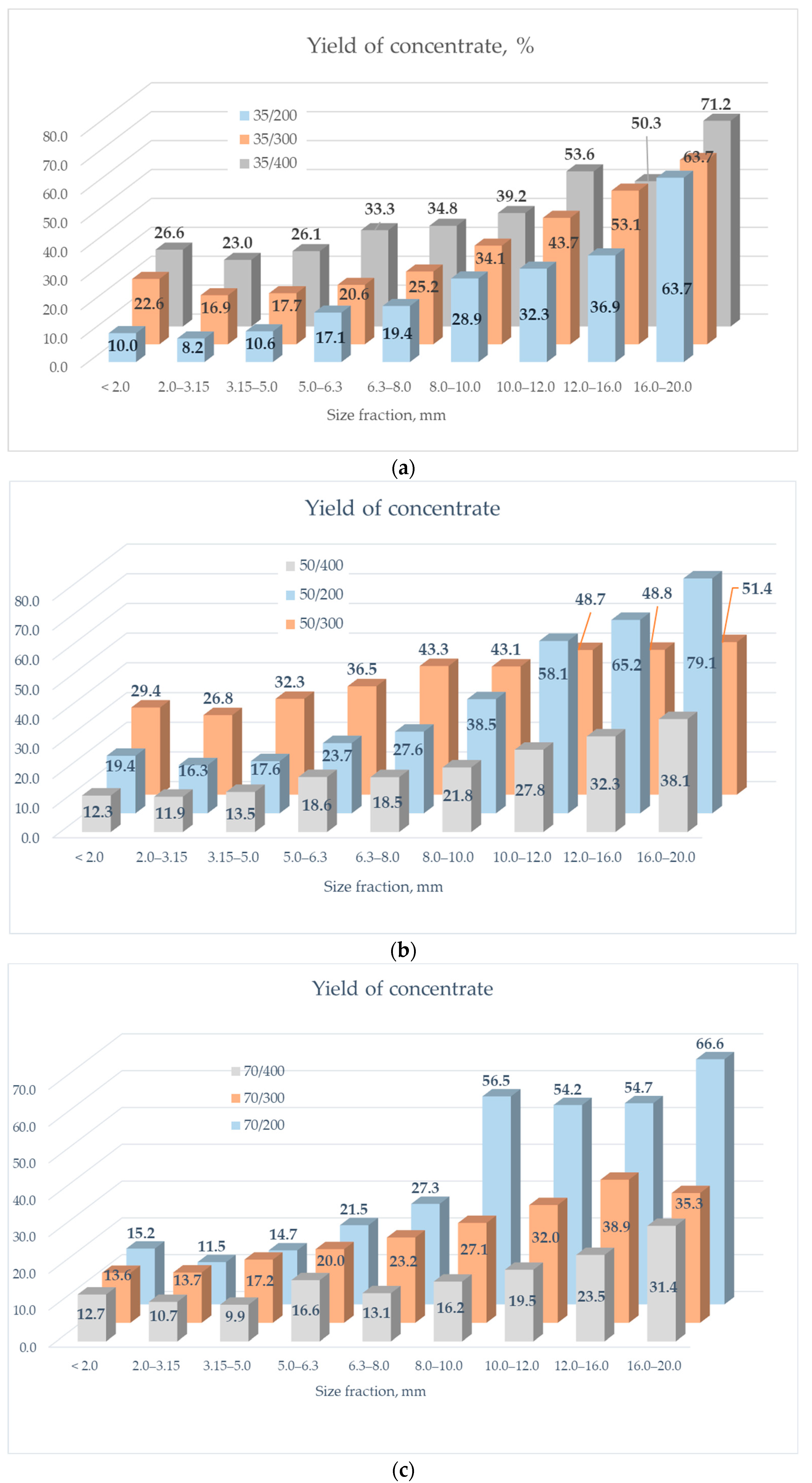
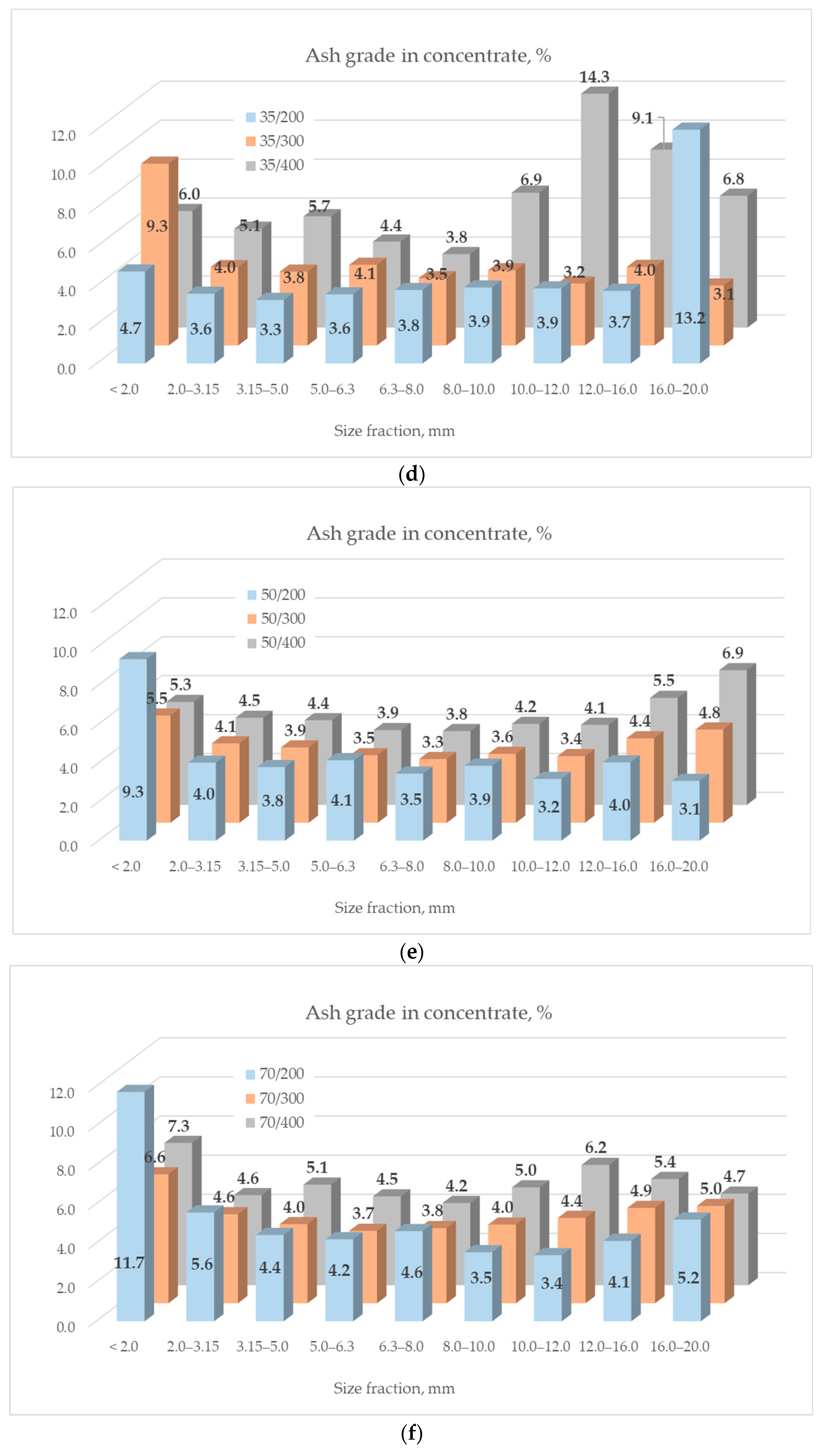
Figure 2 shows the yield of concentrates and the ash grade in the concentrate of products obtained from the experiments for individual particle size fractions. It was observed that the yield of concentrates enhanced by increasing the particle size. A particularly clear boost in the yield of concentrate for fractions above 8 mm was observed for the experiment with the lowest capacity of 200 t/h and the largest amount of hutch water 70 m3/h (Figure 2c). In experiments with the capacity of 200 t/h and the smallest amount of additional water, the yield was improved together with the increase in particle size and reached a value above 60% for the coarsest particles of 16.0–20.0 mm (Figure 2a), while for 50 m3/h of additional water, the yield above 50% could be observed for particles above 10 mm (Figure 2b). For higher yields of concentrate, the highest values were detected in the coarsest fractions of 12.0–16.0 mm (Figure 2a) and 16.0–20.0 mm (Figure 2b). By analyzing the quality of concentrates, an increase in ash in the finest fraction < 2.0 mm (Figure 2e,f) and in the coarsest fraction > 16.0 mm could be seen in the case of the lowest capacity (Figure 2d). In the remaining cases of variable capacity and the amount of additional water, the ash grade in the concentrate remained at a constant level.

3.1. Kruskal–Wallis Test for Yield Depending on the Amount of Hutch Water and System Capacity

First, for each particle size fraction, the Kruskal–Wallis test was performed in relation to the yield depending on the amount of hutch water and the system capacity using Equation (3). The assumptions of the test were met. The test was carried out for each amount of hutch water considered, as well as the yield.
The example of test results is presented in Table 1. The other ones can be found in Appendix A (Table A1, Table A2, Table A3, Table A4 and Table A5).
The H statistics had a distribution of χ 2 with (k − 1) degrees of freedom (k = 3). The critical value for the significance level = 0.05 was χ 2 = 5.991. Since in each case H < χ 2 there were no grounds for rejecting the H0 hypothesis, it could be assumed that the yield in individual particle size fractions, regardless of the amount of hutch water added and the system capacity, was subjected to the same distributions.

3.2. Friedman’s Test for the Yield Depending on the Hutch Water Amount and Capacity

Similarly, as described in Section 3.2, an analysis was carried out for the yield depending on the added hutch water and system capacity using the Friedman test. Equation (4) was used for this purpose. The example of the test results is shown in Table 2. The rest of the results are positioned in Appendix A (Table A6, Table A7, Table A8, Table A9 and Table A10).
Analyzing the results of the Friedman test showed that in most cases there is no reason to reject the null hypothesis. However, in the case of particle size fraction (16.00–20.00 mm) at u = 35 m3/h, size fraction (8.00–10.00 mm) at u = 70 m3/h and fractions (8.00–10.00 mm) at v = 200 ton/h, the test values exceeded the critical value χ2, which indicated that in these cases the H0 hypothesis should be rejected.

3.3. Friedman Test for Two Subgroups of Coal Density Fractions

When analyzing the height of the ranks assigned to the results obtained in Section 3.2., it can be observed that in fractions with low densities, low ranks had results that corresponded to particles of coarser size. An inverse relationship can be observed for fractions with higher densities. Therefore, to examine this relationship, the Friedman test was carried out separately for the fractions corresponding to the density ranges (1.20–1.70 g/cm3) and (1.50–2.20 g/cm3). The test results are presented in Table 3 and the remaining outcomes are positioned in Appendix A (Table A11, Table A12, Table A13, Table A14 and Table A15).
R11, R12 and R13 are rank sums including density fractions (1.20–1.70 g/cm3) and R21, R22 and R23 are rank sums including density fractions (1.50–2.20 g/cm3); χ 1 2 —test value for the density range (1.20–1.70 g/cm3),   χ 2 2 —test value for the density range (1.50–2.20 g/cm3).
Analyzing the obtained results of the Friedman test for the two subgroups of density fractions, it can be seen that in a large number of cases, the hypothesis of the same distributions of concentrate output should be rejected. Thus, in these subgroups the distribution of the material depends on both variables, i.e., u (the amount of hutch water) and v (system capacity).
With fixed u values, greater differences occurred in the group with higher densities. If u = 35 m3/h, then in group I only in one case the H0 hypothesis should be rejected. In group II, H0 should be rejected in four cases. If u = 50 m3/h, the hypothesis was rejected in group I in two cases and in group II in six cases. If, on the other hand, u = 70 m3/h, then in group I the H0 hypothesis was not rejected even once, while in group II it was rejected in three cases.
A similar situation can be observed in the case of determining the level of the variable v. If v = 200 t/h, the hypothesis H0 was not rejected in group I in any case, and in group II it was rejected in one case. If v = 300 t/h, then in group I the null hypothesis should be rejected in three cases, and in group II it should also be rejected in three cases. If v = 400 t/h, then in group I the H0 hypothesis was not rejected even once, and in group II it was rejected in two cases.
The above studies and considerations show that both the amount of hutch water and the capacity of the system have an impact on the discharge size distribution, along with the fact that the influence of these factors was smaller in the case of the fraction with a lower density, and greater in the case of the fraction with a higher density.

3.4. The Friedman Test for Ash Grade

The dependence of ash grade in particle size fractions on the values of u and v was also examined using the Friedman test.
The results of the analyses are presented in Table 4 and Table 5.
Analyzing the results of the Friedman test for the relationship between the ash grade in coal concentrate particle size fractions and variables u and v, it can be seen that in no case did the test value exceed the critical value χ2 = 5.991 (for the significance level α = 0.05), so there are no grounds for the rejection of hypothesis H0. It can therefore be concluded that the dependence of the ash grade on both the amount of hutch water and the capacity of the system is low.

4. Conclusions

The criteria determining the usability of the fuel involve creating the possibility of the most perfect purification of raw coal, i.e., complete separation of gangue from the target material and removal of the largest possible amount of free particles of pyritic sulfur. Classic gravitational beneficiation methods are the cheapest way to improve the quality of the produced assortments. However, the degree of removal of ash and sulfur from coal enriched with these methods varies. In the presented article, a new approach was proposed to assess the quality of beneficiation products in a jig. Using the Kruskal–Wallis and Friedman tests, the influence of the amount of hutch water and the capacity of the system on the yield of concentrate was assessed, considering specific density–size fractions. The applied mathematical methods allowed for the reliable assessment of the impact of variable process conditions on the assessment of the quality of the final product. The described methodology can be used in the assessment of any enrichment process for various types of raw materials and various types of process factors, and does not need to fulfill the required assumptions necessary to conduct ANOVA analysis.
The results of the Friedman test indicated that if only low-density fractions were considered, the influences of hutch water amount and system capacity on yield distribution in these fractions were not significant. For higher density fractions, this influence became significant. Therefore, it was possible to select the optimal values of the considered factors which did not matter with regard to ash grade distribution.
The methodology of the elaborate experiments presented in this paper is original and different to traditional approaches used to evaluate the jigging process. It allows one to look more widely at the results of coal separation. The applied tools such as the Kruskal–Wallis and Friedman tests served to evaluate the quantity and quality of the jigging process, which can make it easier to forecast the separation results with regard to the production of commercial products fulfilling certain needs of recipients.

Author Contributions

Conceptualization, writing—original draft and writing—review and editing, T.N. and A.S.; methodology, validation and formal analysis, T.N.; investigation, resources and data curation, A.S.; writing—review and editing and supervision, A.H. and H.K. All authors have read and agreed to the published version of the manuscript.

Funding

This research received no external funding.

Data Availability Statement

The data presented in this study are available on request from the corresponding author. The data are not publicly available due to ethical restrictions.

Conflicts of Interest

The authors declare no conflict of interest.

Appendix A

Table A1. The Kruskal–Wallis test results for yield (u = 50); Ri = sum of ranks for v = 200 t/h (R1), 300 t/h (R2) and 400 t/h (R3).
Particle Size Fraction [mm]vH
R1R2R3
0.00–2.0070.0119.0111.03.220
2.00–3.1571.0125.0104.03.730
3.15–5.0071.0124.0105.03.600
5.00–6.3071.0124.0105.03.600
6.30–8.0070.0122.0108.03.620
8.00–10.0075.0110.0115.02.375
10.00–12.0079.0103.0118.01.935
12.00–16.0085.097.0118.01.395
16.00–20.0078.099.0123.02.535
Table A2. The Kruskal–Wallis test results for yield (u = 70); Ri = sum of ranks for v = 200 t/h (R1), 300 t/h (R2) and 400 t/h (R3).
Particle Size Fraction [mm]vH
R1R2R3
0.00–2.00112.085.0103.00.945
2.00–3.1592.098.0110.00.420
3.15–5.0092.595.0112.50.593
5.00–6.3084.0108.0108.00.960
6.30–8.0090.094.0116.00.980
8.00–10.0080.0100.0120.02.000
10.00–12.0085.593.0121.51.803
12.00–16.0088.0102.0110.00.620
16.00–20.0084.0104.5111.51.020
Table A3. The Kruskal–Wallis test results for yield (v = 200); Ri = sum of ranks for u = 35 m3/h (R1), 50 m3/h (R2) and 70 m3/h (R3).
Particle Size Fraction [mm]uH
R1R2R3
0.00–2.00108.078.0114.01.860
2.00–3.15112.084.0104.03.000
3.15–5.00117.083.0100.01.445
5.00–6.30119.579.5101.02.005
6.30–8.00122.082.096.02.060
8.00–10.00124.095.081.02.405
10.00–12.00116.088.095.00.560
12.00–16.00126.086.088.02.540
16.00–20.00115.090.095.00.875
Table A4. The Kruskal–Wallis test results for yield (v = 300); Ri = sum of ranks for u = 35 m3/h (R1), 50 m3/h (R2) and 70 m3/h (R3).
Particle Size Fraction [mm]uH
R1R2R3
0.00–2.00101.0128.071.04.065
2.00–3.15101.0127.072.03.785
3.15–5.00102.0124.074.03.140
5.00–6.30103.0118.079.01.935
6.30–8.00113.0113.074.02.535
8.00–10.00116.0106.078.01.940
10.00–12.00120.095.085.00.625
12.00–16.00120.097.083.01.745
16.00–20.00120.096.084.01.680
Table A5. The Kruskal–Wallis test results for yield (v = 400); Ri = sum of ranks for u = 35 m3/h (R1), 50 m3/h (R2) and 70 m3/h (R3).
Particle Size Fraction [mm]uH
R1R2R3
0.00–2.00107.0111.082.01.235
2.00–3.15104.0112.084.01.604
3.15–5.0099.0111.090.00.555
5.00–6.30116.0100.084.01.280
6.30–8.00103.096.0101.00.065
8.00–10.00109.0104.087.00.665
10.00–12.00101.0102.097.00.035
12.00–16.00123.097.080.02.345
16.00–20.00103.0115.082.01.395
Table A6. The Friedman test results, u = 50 m3/h.
Particle Size Fraction [mm]vχ2
R1R2R3
0.00–2.0013.017.018.01.750
2.00–3.1512.017.019.03.250
3.15–5.0013.017.018.01.750
5.00–6.3012.017.019.03.250
6.30–8.0012.017.019.03.250
8.00–10.0012.016.020.04.000
10.00–12.0015.013.020.03.250
12.00–16.0013.014.021.04.750
16.00–20.0014.014.020.04.000
Table A7. The Friedman test results, u = 70 m3/h.
Particle Size Fraction [mm]vχ2
R1R2R3
0.00–2.0020.013.015.03.250
2.00–3.1514.015.019.01.750
3.15–5.0013.514.020.03.060
5.00–6.3014.014.020.03.000
6.30–8.0011.016.021.03.000
8.00–10.0012.015.021.06.250
10.00–12.0011.018.019.05.250
12.00–16.0011.516.519.04.750
16.00–20.0011.516.520.04.560
Table A8. The Friedman test results, v = 200 t/h.
Particle Size Fraction [mm]uχ2
R1R2R3
0.00–2.0018.011.019.04.750
2.00–3.1518.012.018.03.000
3.15–5.0019.013.016.02.250
5.00–6.3020.011.017.05.250
6.30–8.0020.012.016.04.000
8.00–10.0022.015.011.07.750
10.00–12.0035.020.012.04.000
12.00–16.0021.013.014.04.750
16.00–20.0019.014.015.01.750
Table A9. The Friedman test results, v = 300 t/h.
Particle Size Fraction [mm]uχ2
R1R2R3
0.00–2.0019.017.012.03.250
2.00–3.1518.018.012.03.000
3.15–5.0018.017.013.01.750
5.00–6.3017.016.015.00.250
6.30–8.0019.016.013.02.250
8.00–10.0019.015.014.01.750
10.00–12.0021.013.014.04.750
12.00–16.0020.012.016.04.000
16.00–20.0020.012.016.04.000
Table A10. The Friedman test results, v = 400 t/h.
Particle Size Fraction [mm]uχ2
R1R2R3
0.00–2.0013.020.015.03.250
2.00–3.1516.018.014.01.000
3.15–5.0014.018.016.01.000
5.00–6.3018.016.014.01.000
6.30–8.0016.013.019.02.250
8.00–10.0017.015.016.00.250
10.00–12.0015.017.016.00.250
12.00–16.0020.015.013.03.250
16.00–20.0016.019.013.02.250
Table A11. The Friedman test results, u = 50 m3/h, divided into two subgroups.
Particle Size Fraction [mm]Vv χ 1 2 χ 2 2
R11R12R13R21R22R23
0.00–2.0010.08.012.05.014.011.01.6008.400
2.00–3.159.08.013.05.014.011.02.8008.400
3.15–5.0010.08.012.05.014.011.01.6008.400
5.00–6.309.08.013.05.014.011.02.8008.400
6.30–8.009.08.013.05.014.011.02.8008.400
8.00–10.009.07.014.05.013.012.05.2007.600
10.00–12.0012.05.013.07.010.013.07.6003.600
12.00–16.0010.06.014.06.011.013.06.4003.600
16.00–20.0010.07.013.06.011.013.03.6005.200
Table A12. The Friedman test results, u = 70 m3/h, divided into two subgroups.
Particle Size Fraction [mm]vv χ 1 2 χ 2 2
R11R12R13R21R22R23
0.00–2.0012.010.08.014.07.09.01.6005.200
2.00–3.1511.019.010.07.09.014.00.4005.200
3.15–5.0010.09.011.07.58.514.00.4004.900
5.00–6.3010.09.011.07.08.015.00.4007.600
6.30–8.0010.09.011.08.08.014.00.4004.800
8.00–10.007.010.013.06.010.014.03.6006.400
10.00–12.008.010.012.06.010.014.01.6006.400
12.00–16.007.511.511.06.011.013.01.9005.200
16.00–20.007.012.011.06.59.514.05.2005.700
Table A13. The Friedman test results, v = 200 t/h, divided into two subgroups.
Particle Size Fraction [mm]uu χ 1 2 χ 2 2
R11R12R13R21R22R23
0.00–2.0011.07.012.012.06.012.02.8004.800
2.00–3.1510.08.012.012.07.011.01.6002.800
3.15–5.0010.08.012.014.07.09.01.6005.200
5.00–6.3012.07.011.014.06.010.02.8006.400
6.30–8.0011.08.011.015.06.09.01.2008.400
8.00–10.0013.09.08.015.09.06.02.8008.400
10.00–12.0012.07.011.014.08.09.02.8008.400
12.00–16.0012.08.010.015.07.08.01.6007.600
16.00–20.0012.08.010.013.09.08.01.6002.800
R11, R21 mean the sum of ranks in individual subgroups for u = 35 m3/h; R12, R22 are the sum of ranks in individual subgroups for u = 50 m3/h and R13, R23 mean the sum of ranks in individual subgroups for u = 70 m3/h.
Table A14. The Friedman test results, v = 300 t/h, divided into two subgroups.
Particle size Fraction [mm]uu χ 1 2 χ 2 2
R11R12R13R21R22R23
0.00–2.0013.08.09.011.014.05.02.8008.400
2.00–3.1512.09.09.011.014.05.01.2008.400
3.15–5.0012.08.010.05.012.013.01.6007.600
5.00–6.3011.07.012.010.013.07.02.8003.600
6.30–8.0013.07.010.011.013.06.03.6005.200
8.00–10.0013.06.011.012.012.06.05.2004.800
10.00–12.0014.05.011.013.010.07.08.4003.600
12.00–16.0013.05.012.013.09.08.07.6002.800
16.00–20.0013.05.012.013.09.08.07.6004.400
Table A15. The Friedman test results, v = 400 t/h, divided into two subgroups.
Particle Size Fraction [mm]uu χ 1 2 χ 2 2
R11R12R13R21R22R23
0.00–2.006.012.012.010.014.06.04.8006.400
2.00–3.158.011.011.012.012.06.01.2004.800
3.15–5.008.010.012.09.012.09.01.6001.600
5.00–6.309.011.010.013.09.08.00.4001.400
6.30–8.008.09.013.011.07.012.02.8002.800
8.00–10.0010.010.010.013.09.08.00.0002.800
10.00–12.007.011.012.011.010.09.02.8000.400
12.00–16.0011.010.09.015.09.06.00.4008.400
16.00–20.009.012.09.011.012.07.01.2002.800

References

  1. Stępiński, W. Krzywe średnich wartości. Rudy Met. Nieżelazne 1965, 9, 532–535. (In Polish) [Google Scholar]
  2. Brożek, M. Ocena stopnia uwolnienia frakcji mineralnej węgla na podstawie krzywej separacji Halla. Prz. Górniczy 1984, 11, 384–387. (In Polish) [Google Scholar]
  3. Niedoba, T. Ocena zawartości popiołu w pokładach węgla za pomocą nieparametrycznych metod statystycznych. Górnictwo I Geoinżynieria 2007, 4, 39–50. (In Polish) [Google Scholar]
  4. Niedoba, T. Wielowymiarowe Charakterystyki Zmiennych Losowych W Opisie Materiałów Uziarnionych I Procesów Ich Rozdziału; IGSMiE PAN: Krakow, Poland, 2013. (In Polish) [Google Scholar]
  5. Tumidajski, T. Zastosowanie Metod Statystycznych W Analizie Procesów Przeróbki Surowców Mineralnych; Śląskie Wydawnictwo Naukowe: Krakow, Poland, 1993. (In Polish) [Google Scholar]
  6. Niedoba, T.; Jamróz, D. Visualization of multidimensional data in purpose of qualitative classification of various types of coal. Arch. Min. Sci. 2013, 58, 1317–1333. [Google Scholar]
  7. Niedoba, T. Statistical analysis of the relationship between particle size and particle density of raw coal. Physicochem. Probl. Miner. Process. 2013, 49, 175–188. [Google Scholar]
  8. Surowiak, A.; Foszcz, D.; Niedoba, T. Evaluation of jig work on the basis of granulometric analysis of particle size fractions of beneficiation products in purpose of process optimization. IOP Conf. Ser.-Mat. Sci. 2019, 641, 012006. [Google Scholar]
  9. Niedoba, T. Wielowymiarowe rozkłady charakterystyk materiałów uziarnionych przy zastosowaniu nieparametrycznych aproksymacji funkcji gęstości rozkładów brzegowych. Górnictwo I Geoinżynieria 2009, 33, 235–244. (In Polish) [Google Scholar]
  10. Niedoba, T.; Pięta, P.; Surowiak, A. Factor Analysis and Mathematical Modeling in Determining the Quality of Coal. Inz. Miner. 2020, 22, 151–160. [Google Scholar] [CrossRef]
  11. Jamróz, D.; Niedoba, T. Application of Observational Tunnels Method to Select Set of Features Sufficient to Identify a Type of Coal. Physicochem. Probl. Miner. Process. 2014, 50, 185–202. [Google Scholar]
  12. Niedoba, T. Multi-parameter data visualization by means of principal component analysis (PCA) in qualitative evaluation of various coal types. Physicochem. Probl. Miner. Process. 2014, 50, 575–589. [Google Scholar]
  13. Jamróz, D.; Niedoba, T.; Surowiak, A.; Tumidajski, T. The use of the visualisation of multidimensional data using PCA to evaluate possibilities of the division of coal samples space due to their suitability for fluidised gasification. Arch. Min. Sci. 2016, 61, 523–535. [Google Scholar] [CrossRef]
  14. Niedoba, T. Application of relevance maps in multidimensional classification of coal types. Arch. Min. Sci. 2015, 60, 93–106. [Google Scholar]
  15. Jamróz, D.; Niedoba, T. Application of multidimensional data visualization by means of self-organizing Kohonen maps to evaluate classification possibilities of various coal types. Arch. Min. Sci. 2015, 60, 39–50. [Google Scholar]
  16. Jamróz, D. Application of multidimensional scaling to classification of various types of coal. Arch. Min. Sci. 2014, 59, 413–425. [Google Scholar]
  17. Jamróz, D. Application of multi-parameter data visualization by means of autoassociative neural networks to evaluate classification possibilities of various coal types. Physicochem. Probl. Miner. Process. 2014, 50, 719–734. [Google Scholar]
  18. Jamróz, D.; Niedoba, T. Comparison of selected methods of multi-parameter data visualization used for classification of coals. Physicochem. Probl. Miner. Process. 2015, 51, 769–784. [Google Scholar]
  19. Surowiak, A. Assessment of coal mineral matter liberation efficiency index. Inz. Miner. 2013, 14, 153–158. [Google Scholar]
  20. Cierpisz, S.; Joostberens, J. Monitoring of coal separation in a jig using a radiometric density meter. Measurement 2016, 88, 147–152. [Google Scholar] [CrossRef]
  21. Cierpisz, S. A dynamic model of coal products discharge in a jig. Miner. Eng. 2017, 105, 1–6. [Google Scholar] [CrossRef]
  22. Cierpisz, S.; Kryca, M.; Sobierajski, W. Control of coal separation in a jig using a radiometric meter. Miner. Eng. 2016, 95, 59–65. [Google Scholar] [CrossRef]
  23. Dong, K.J.; Kuang, S.B.; Vince, A.; Hughes, T.; Yu, A.B. Numerical simulation of the in-line pressure jig unit in coal preparation. Miner. Eng. 2010, 23, 301–312. [Google Scholar] [CrossRef]
  24. Constant, M.; Coppin, N.; Dubois, F.; Artoni, R.; Lambrechts, J.; Legat, V. Numerical investigation of the density sorting of grains using water jigging. Powder Technol. 2021, 393, 705–721. [Google Scholar] [CrossRef]
  25. Ferreira Feil, N.; Sampaio, C.H.; Wotruba, H. Influence of jig frequency on the separation of coal from the Bonito-seam—Santa Catarina, Brazil. Fuel Process. Technol. 2012, 96, 22–26. [Google Scholar] [CrossRef]
  26. Tripathy, A.; Panda, L.; Sahoo, A.K.; Biswal, S.K.; Dwari, R.K.; Sahu, A.K. Statistical optimization study of jigging process on beneficiation of fine size high ash Indian non-coking coal. Adv. Powder Technol. 2016, 27, 1219–1224. [Google Scholar] [CrossRef]
  27. Panda, L.; Sahoo, A.K.; Tripathy, A.; Biswal, S.K.; Sahu, A.K. Application of artificial neural network to study the performance of jig for beneficiation of non-coking coal. Fuel 2012, 97, 151–156. [Google Scholar] [CrossRef]
  28. Khoshdast, H.; Soflaeian, A.; Shojaei, V. Coupled fuzzy logic and experimental design application for simulation of a coal classifier in an industrial environment. Physicochem. Probl. Miner. Process. 2019, 55, 504–515. [Google Scholar]
  29. Jarkani, S.A.; Khoshdast, H.; Shariat, E.; Sam, A. Modeling the effects of mechanical parameters on the hydrodynamic behavior of vertical current classifiers. Int. J. Min. Sci. Technol. 2014, 24, 123–127. [Google Scholar] [CrossRef]
  30. Kumar, S.; Venugopal, R. Coal cleaning using jig and response surface approach for determination of quality of clean coal. Int. J. Coal Prep. Util. 2020, 40, 107–115. [Google Scholar] [CrossRef]
  31. Xia, Y.; Peng, F.F.; Wolfe, E. CFD simulation of fine coal segregation and stratification in jigs. Int. J. Miner. Process. 2007, 82, 164–176. [Google Scholar] [CrossRef]
  32. Khoshdast, H.; Shojaei, V.; Khoshdast, H. Combined application of computational fluid dynamics (CFD) and design of experiments (DOE) to hydrodynamic simulation of a coal classifier. Int. J. Min. Geo-Eng. 2017, 51, 9–24. [Google Scholar]
  33. Ma, F.Q.; Liu, X.W.; Tan, D.J. Jigging process human-like intelligent control. In Proceedings of the 4th World Congress of Intelligent Control and Automation, Shanghai, China, 10–14 June 2002. [Google Scholar]
  34. Gouri Charan, T.; Chattopadhyay, U.S.; Singh, K.M.P.; Kabiraj, S.K.; Haldar, D.D. Beneficiation of high-ash, Indian non-coking coal by dry jigging. Miner. Metall. Explor. 2011, 28, 21–23. [Google Scholar] [CrossRef]
  35. Sampaio, C.H.; Aliaga, W.; Pacheco, E.T.; Petter, E.; Wotruba, H. Coal beneficiation of Candiota mine by dry jigging. Fuel Process. Technol. 2008, 89, 198–202. [Google Scholar] [CrossRef]
  36. Yang, X.; Zhao, Y.; Luo, Z.; Song, S.; Duan, C.; Dong, L. Fine coal dry cleaning using a vibrated gas-fluidized bed. Fuel Process. Technol. 2013, 106, 338–343. [Google Scholar] [CrossRef]
  37. Mohanty, M.K.; Honaker, R.Q.; Patwardhan, A. Altair jig: An in-plant evaluation for fine coal cleaning. Miner. Eng. 2002, 15, 157–166. [Google Scholar] [CrossRef]
  38. Richards, R.G.; Jones, T.A. Kelsey centrifugal jig—An update on technology and application. Miner. Metall. Process. 2004, 21, 179–182. [Google Scholar] [CrossRef]
  39. Mishra, B.K.; Adhikari, B. Analysis of fluid motion during jigging. Miner. Eng. 1999, 12, 1469–1477. [Google Scholar] [CrossRef]
  40. Kuang, Y.L.; Ou, Z.S. Mathematic simulation of water motion in jig. In Proceedings of the 5th International Symposium on Mining Science and Technology (ISMST), Xuzhou, China, 20–22 October 2004. [Google Scholar]
  41. Phengsaart, T.; Ito, M.; Hamaya, N.; Tabelin, C.B.; Hiroyoshi, N. Improvement of jig efficiency by shape separation and a novel method to estimate the separation efficiency of metal wires in crushed electronic wastes using bending behavior and “entanglement factor”. Miner. Eng. 2018, 129, 54–62. [Google Scholar] [CrossRef]
  42. Surowiak, A.; Gawenda, T.; Stempkowska, A.; Niedoba, T.; Nad, A. The influence of selected properties of particles in the jigging process of aggregates on an example of chalcedonite. Minerals 2020, 10, 600. [Google Scholar] [CrossRef]
  43. Venkoba Rao, B.; Jeelan, G.; Shirke, S.; Gopalkrishna, S.J. Experimental validation of extended stratification model part B: Coal-ash segregation studies in a batch jig operation. Trans. Indian Inst. Metals 2017, 70, 375–394. [Google Scholar] [CrossRef]
  44. Gagarin, S.G.; Gyul’maliev, A.M.; Tolchenkin, Y.A. Trends in Coal Beneficiation: A Review. Coke Chem. 2008, 51, 31–42. [Google Scholar] [CrossRef]
  45. Mukherjee, A.K.; Dwivedi, V.K.; Mishra, B.K. Analysis of a laboratory jigging system for improved performance. Miner. Eng. 2005, 18, 1037–1044. [Google Scholar] [CrossRef]
  46. Paul, S.R.; Bhattacharya, S. Size by size separation characteristics of a coal cleaning jig. Trans. Indian Inst. Met. 2018, 71, 1439–1444. [Google Scholar] [CrossRef]
  47. Lyman, G.J. Review of Jigging Principles and Control. Coal Prep. 1992, 11, 145–165. [Google Scholar] [CrossRef]
  48. Wills, B.A.; Finch, J. Mineral Processing Technology. An Introduction to the Practical Aspects of Ore Treatment and Mineral Recovery; Elsevier: Oxford, UK, 2006. [Google Scholar]
  49. Surowiak, A. The analysis of coal fines separation precision exposed to changeable hydrodynamic parameters of jig work. Arch. Min. Sci. 2018, 63, 437–448. [Google Scholar]
  50. Surowiak, A. Investigation and evaluation of jigging separation features. Arch. Min. Sci. 2018, 63, 839–851. [Google Scholar]
  51. Surowiak, A. Evaluation of fine coal upgrading effects by means of Fuerstenau curves. Gospod. Surowcami Min. 2019, 35, 5–24. [Google Scholar]
  52. Surowiak, A.; Foszcz, D.; Niedoba, T. Optimisation of coal beneficiation in a jig in changing hydrodynamic conditions of its operation. Acta Montan. Slovaca 2022, 27, 1–10. [Google Scholar]
  53. Hori, K.; Tsunekawa, M.; Hiroyoshi, N.; Ito, M. Optimum water pulsation of jig separation for crushed plastic particles. Int. J. Miner. Process. 2009, 92, 103–108. [Google Scholar] [CrossRef]
  54. Osoba, M. Polskie osadzarki wodne pulsacyjne do wzbogacania surowców mineralnych. Inz. Miner. 2014, 2, 287–294. (In Polish) [Google Scholar]
  55. Blaschke, W. Technologie Czystego Węgla rozpoczynają się od jego wzbogacania. Polityka Energ. 2008, 11, 7–13. (In Polish) [Google Scholar]
  56. Niedoba, T.; Pięta, P. Applications of ANOVA in mineral processing. Min. Sci. 2016, 23, 43–54. [Google Scholar]
  57. Niedoba, T.; Surowiak, A.; Pięta, P. Application of variance analysis to compare characteristics of various types of hard coal. Inz. Miner. 2016, 17, 15–22. [Google Scholar]
  58. Murakami, H.; Lee, S.K. Unbiasedness and biasedness of the Jonckheere-Terpstra and the Kruskal-Wallis tests. J. Korean Stat. Soc. 2015, 44, 342–351. [Google Scholar] [CrossRef]
  59. Duris, V.; Tirpakova, A. A survey on the global optimization problem using Kruskal-Wallis test. Ann. Math. Inform. 2020, 52, 281–298. [Google Scholar]
  60. Liu, Y.W.; Chen, W.H. A SAS Macro for Testing Differences among Three or More Independent Groups Using Kruskal-Wallis and Nemenyi Tests. J. Huazhong Univ. Sci. Technol. Med. Sci. 2012, 32, 130–134. [Google Scholar] [CrossRef]
  61. Van Hecke, T. Power study of ANOVA versus Kruskal-Wallis test. J. Stat. Manag. Syst. 2012, 15, 241–247. [Google Scholar]
  62. Lachenbruch, P.A.; Clements, P.J. ANOVA, Kruskal-Wallis, Normal Scores and Unequal Variance. Commun. Stat. 1991, 20, 107–126. [Google Scholar] [CrossRef]
  63. Ferreira, E.B.; Rocha, M.C.; Mequelino, D.B. Monte Carlo evaluation of the ANOVA’s F and Kruskal-Wallis tests under binomial distribution. Sigmae 2012, 1, 126–139. [Google Scholar]
  64. Baer, A.; Lawonn, K.; Saalfeld, P.; Preim, B. Statistical Analysis of a Qualitative Evaluation on Feature Lines. In Proceedings of the Bildverarbeitung Fur Die Medizin 2015: Algorithmen—Systeme—Anwendungen 2015, Lübeck, Germany, 15–17 March 2015. [Google Scholar]
  65. Guo, S.X.; Zhong, S.; Zhang, A.D. Privacy-preserving Kruskal-Wallis test. Comput. Methods Programs Biomed. 2013, 112, 135–145. [Google Scholar] [CrossRef]
  66. Vargha, A.; Delaney, H.D. The Kruskal-Wallis test and stochastic homogeneity. J. Educ. Behav. Stat. 1998, 23, 170–192. [Google Scholar] [CrossRef]
  67. Sherwani, R.A.K.; Shakeel, H.; Awan, W.B.; Faheem, M.; Aslam, M. Analysis of COVID-19 data using neutrosophic Kruskal Wallis H test. BMC Med. Res. Methodol. 2021, 21, 215. [Google Scholar] [CrossRef] [PubMed]
  68. Dobosz, M. Wspomagana Komputerowo-Statystyczna Analiza Wyników Badań; Akademicka Oficyna Wydawnicza EXIT: Warszawa, Poland, 2001. (In Polish) [Google Scholar]
  69. Stanisz, A. Przystępny Kurs Statystyki, Tom II; Statsoft: Krakow, Poland, 2007. (In Polish) [Google Scholar]
  70. Wayne, W.W. Applied Nonparametric Statistics; PWS-Kent: Boston, MA, USA, 1990. [Google Scholar]
  71. Friedman, M. The Use of Ranks to Avoid the Assumption of Normality Implicit in the Analysis of Variance. J. Am. Stat. Assoc. 1937, 32, 675–701. [Google Scholar] [CrossRef]
Figure 1. The model of the factorial experiment.
Energies 16 01600 g001
Figure 2. Yield of concentrate and ash grade in the concentrate according to the size fraction: (a) yield of concentrate - hutch water 35 m3/h, (b) yield of concentrate - hutch water 50 m3/h, (c) yield of concentrate - hutch water 70 m3/h, (d) ash grade - hutch water 35 m3/h, (e) ash grade - hutch water 50 m3/h, (f) ash grade - hutch water 70 m3/h.
Energies 16 01600 g002aEnergies 16 01600 g002b
Table 1. The Kruskal–Wallis test results for yield (u = 35); Ri = sum of ranks for v = 200 t/h (R1), 300 t/h (R2) and 400 t/h (R3).
Particle Size Fraction [mm]vH
R1R2R3
0.00–2.00120.092.097.01.145
2.00–3.1588.0112.0100.00.720
3.15–5.00102.0114.084.01.140
5.00–6.3087.0111.0102.00.735
6.30–8.0086.0120.094.01.580
8.00–10.0078.0120.0102.02.220
10.00–12.0088.0114.597.50.900
12.00–16.0077.0112.0111.00.985
16.00–20.0079.0129.092.03.365
Table 2. The Friedman test results, u = 35 m3/h.
Particle Size Fraction [mm]vχ2
R1R2R3
0.00–2.0012.018.018.03.000
2.00–3.1517.018.013.01.750
3.15–5.0014.021.013.04.750
5.00–6.3016.017.015.00.250
6.30–8.0014.017.017.00.750
8.00–10.0012.021.015.05.250
10.00–12.0014.019.015.01.780
12.00–16.0012.019.017.03.250
16.00–20.0013.022.013.06.750
Table 3. The Friedman test results, u = 35 m3/h, divided into two subgroups.
Particle Size Fraction [mm]vv χ 1 2 χ 2 2
R11R12R13R21R22R23
0.00–2.009.012.09.06.011.013.01.2005.200
2.00–3.1512.012.06.010.011.09.04.8000.400
3.15–5.0011.013.06.07.014.09.05.2005.200
5.00–6.3013.09.08.08.012.010.02.8001.600
6.30–8.0011.08.011.05.014.011.01.2008.400
8.00–10.009.0012.09.05.015.010.01.20010.000
10.00–12.0011.012.07.05.013.012.02.8007.600
12.00–16.009.012.09.08.015.07.02.8007.600
16.00–20.008.013.09.08.015.07.02.8007.600
Table 4. The Friedman test results for the ash grade at a fixed u value (the amount of hutch water).
Particle Size Fraction [mm]u = 35 m3/hu = 50 m3/hu = 70 m3/h
χ2χ2χ2
0.00–2.001.1601.5002.670
2.00–3.150.5002.1700.500
3.15–5.002.1702.6701.170
5.00–6.303.1700.1701.500
6.30–8.002.0505.5002.170
8.00–10.000.6700.1701.500
10.00–12.000.6700.6700.670
12.00–16.000.6700.5002.000
16.00–20.001.5004.5002.000
Table 5. The Friedman test results for ash grade at a fixed value of v (system capacity).
Particle Size Fraction [mm]v = 200 t/hv = 300 t/hv = 400 t/h
χ2χ2χ2
0.00–2.002.6700.6701.500
2.00–3.150.5002.6700.670
3.15–5.000.6702.0004.670
5.00–6.301.5002.0001.170
6.30–8.002.1702.0000.670
8.00–10.001.5002.0000.670
10.00–12.000.6700.6700.670
12.00–16.002.0000.6702.670
16.00–20.000.1250.6704.670
Disclaimer/Publisher’s Note: The statements, opinions and data contained in all publications are solely those of the individual author(s) and contributor(s) and not of MDPI and/or the editor(s). MDPI and/or the editor(s) disclaim responsibility for any injury to people or property resulting from any ideas, methods, instructions or products referred to in the content.

