
Application of the Generalized Normal Distribution Optimization Algorithm to the Optimal Selection of Conductors in Three-Phase Asymmetric Distribution Networks


Abstract
1. Introduction
2. Literature Review and Contributions
- The proposed solution methodology can be implemented for any three-phase balanced and unbalanced distribution system with radial topology regardless of the load connections or the number of buses.
- It’s exploration and exploitation stages make the proposed GNDO a robust and efficient solution methodology, in which with the help vortex search algorithm could obtain an optimal solution in a single evaluation besides using shorter processing times.
- Implementation and adaptation of complementary software such as Microsoft Power BI® allowed us to rigorously examine both technically and economically, the analysis of the algorithm proposed.

| Sol. Methodology | Objetive Function | Operation Scenario | Refs. | Year |
|---|---|---|---|---|
| Evolutionary strategy | Minimize network investment costs | Maximum load on 7-bus system | [14] | 2006 |
| Genetic Algorithms | Minimizing active power losses and maximizing conductor material savings | Maximum load on 13-bus system | [27] | 2011 |
| Harmony search | Minimize the sum of capital investment and energy losses | Heavy load, simulating the agricultural season in a 16 and 85-bus system. | [16] | 2011 |
| Particle swarm optimization | Minimize capital investment depreciation, energy loss costs and maximum current capacity | Maximum load for 26- and 32-bus system | [17,18] | 2012 2016 |
| Modified Differential Evolution | Minimize fixed costs associated with network investment and variable costs associated with operation. | Two scenarios projecting annual load growth | [19] | 2014 |
| Differential evolution | Savings in conductive material costs and energy losses. | Maximum load, implemented in an unbalanced three-phase system of 19 and 34 buses. | [28] | 2016 |
| Crow search algorithm | Minimize capital cost and energy losses | scenario with peak demand in 16- and 85-buses system | [20] | 2017 |
| Sine cosine algorithm | Minimizing the annual cost of energy losses and capital investment | Peak demand, projecting 10 consecutive years of load growth in a 22-buses system. | [21] | 2017 |
| Salp swarm optimizer | Minimize energy losses and investment cost of conductors | Three scenarios at 50, 100 and 150% of nominal load and different levels of distributed generation | [22] | 2018 |
| Improved tabu search algorithm | Minimize investment cost and energy loss | Maximum load on 23-, 48- and 71-buses system | [5] | 2019 |
| Heuristic search method | Driver depression cost and annual energy losses. | Maximum load on 69- and 85-buses system | [23,29] | 2016 2019 |
| Whale optimization algorithm | Minimize the cost of energy loss and investment of conductors | Peak power in 16- and 85-buses system | [24] | 2019 |
| Teaching—learning | Minimize investment and the annual cost of losses | Peak demand scenario in 16-buses system | [25] | 2020 |
| Vortex search algorithm | Minimization of conductor investment costs and network technical losses | Balanced and unbalanced load under three scenarios, at 100% of the maximum load, 50%, and 44% of the nominal load. | [26] | 2021 |
| Newton-based metaheuristic optimizer | minimize annual energy losses and investment in conductors | Balanced and unbalanced load scenarios | [30] | 2022 |
3. Mathematical Formulation
3.1. Objective Function
3.2. Set of Constraints
4. Solution Methodology
4.1. Slave Stage: Three-Phase Power Flow
4.2. Master Stage: GNDO Metaheuristic Algorithm
4.2.1. Local Exploitation
4.2.2. Global Exploration
4.3. Improvement of the Exploration and Exploitation of the Solution Space
Improved Implementation of the GNDO Based on Ellipses of Variable Radius
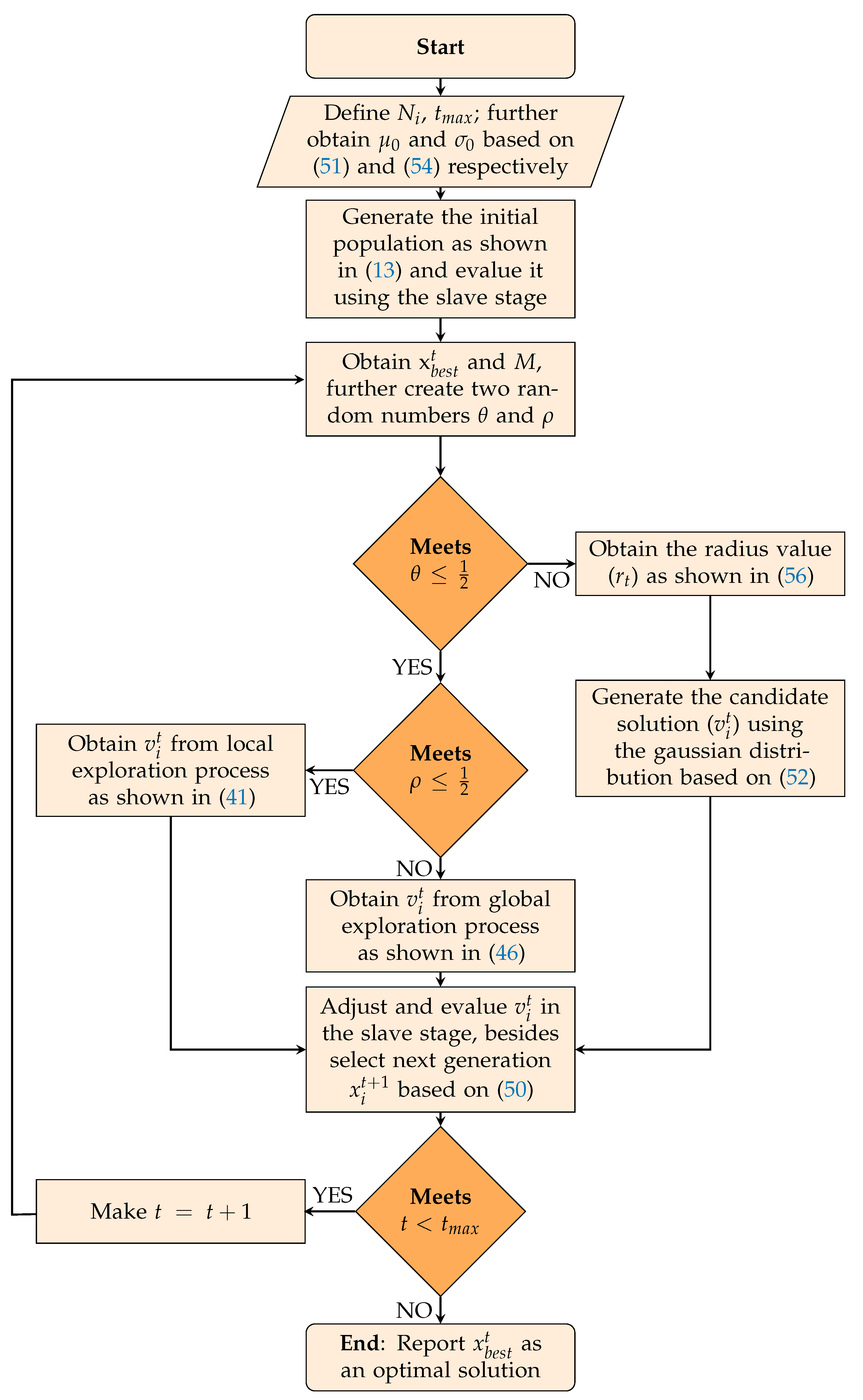
| Algorithm 1. Improved implementation of the GNDO based on the VSA. |
| Select the AC electrical network under study; |
| Find the equivalent electrical network in values per unit; |
| Assign the population size (), the maximum iterations () and ; |
| Find the initial center () and the standard desviation () as shown in (51) and (54), respectively; |
| Generate the initial population according to (13); |
| Establish the best adaptive initial function as () = ∞; |
| do |
| Obtain the value of the objective function for each of the individuals belonging to the initial |
| population with the help of the slave stage; |
| Select the individual as the one that obtains the minimum value in the objective function |
| according to the results found in ; |
| do |
| Generate two random numbers and between 0 and 1; |
| Enter the value of the vector as described in (45); |
| then |
| Generate three random numbers , and with each of them different from each other |
| and different from ; |
| Find the value of and as described in (47) and (48), respectively; |
| then |
| Calculate the value of as described in (42); |
| Obtain the value of as described in (43); |
| Find the penalty factor according to (44); |
| Obtain as described in (41); |
| Perform the global exploration process as explained in (46); |
| Verify and adjust the values of according to the limits established in (49); |
| Evaluate in the slave stage in order to obtain the value of the objective function |
| ; |
| Select next generation as explained in (50); |
| Obtain the radius as expressed in (56); |
| Generate the candidate solutions using the Gaussian distribution with center at |
| based on (52); |
| Verify and adjust the values of according to the limits established in (49); |
| Evaluate in the slave stage in order to obtain the value of the objective function |
| ; |
| Select next generation as explained in (50); |
5. Characteristics of the Test Systems
5.1. First Test System
5.2. Second Test System
5.3. Set of Available Conductors
6. Computational Validation
7. Results and Discussion
7.1. Results in a Balanced Operating Scenario
7.1.1. Results in the IEEE 8-Bus Test System
7.1.2. Results in the IEEE 27-Bus Test Scenario
7.2. Results in an Unbalanced Operating Scenario
7.2.1. Results in the IEEE 8-Bus Test System
7.2.2. Results in the IEEE 27-Bus Test Scenario
7.3. Complementary Analysis
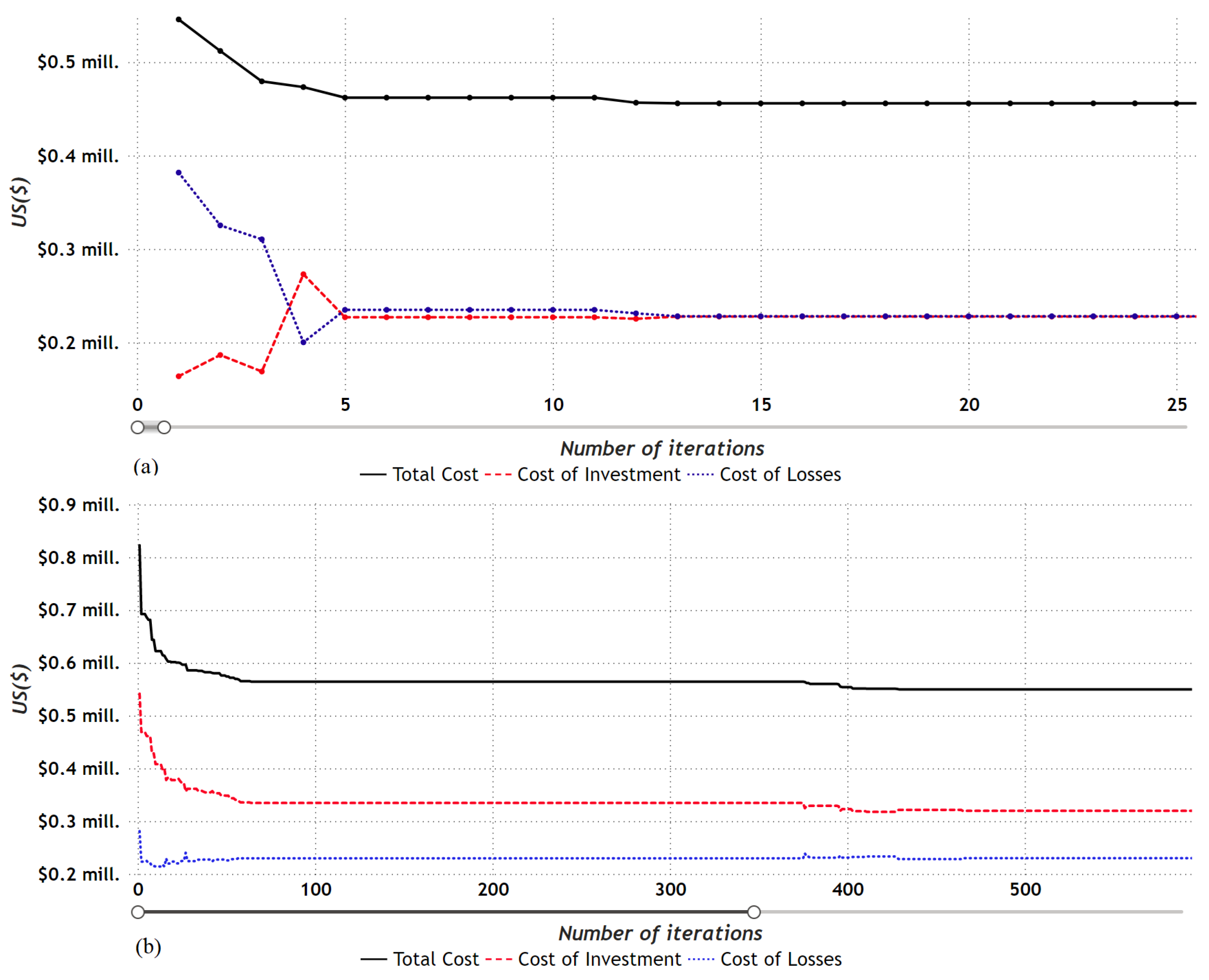
- The proposed GNDO only needs a single evaluation to obtain the numerical results presented in this research, which guarantees very reduced computation times, making this algorithm the most efficient one reported in the specialized literature.
- The proposed GNDO improves the results in most of the case studies presented, with the exception of the 8-bus test system under an unbalanced operating scenario, in which it matches the results obtained by algorithms such as the NMA or the VSA. In this way, it can be inferred that for this particular case study, the overall optimal solution has been obtained.
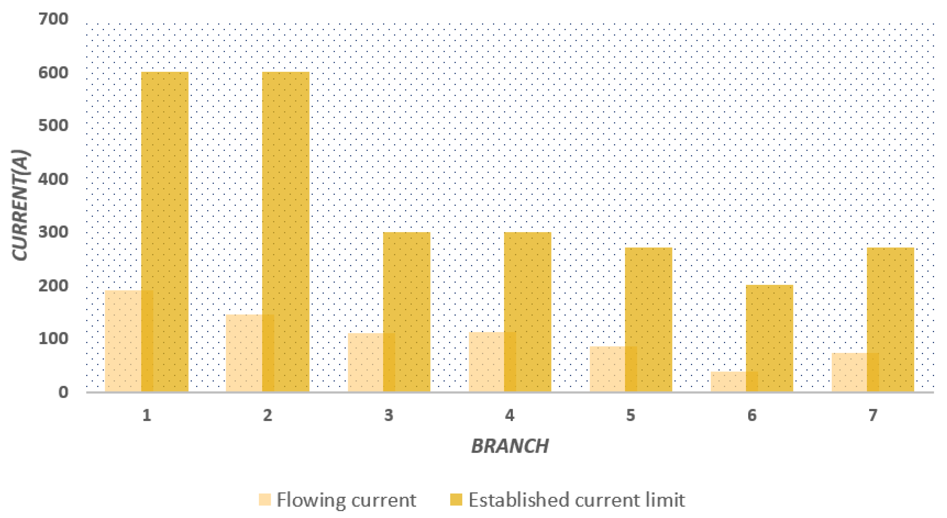
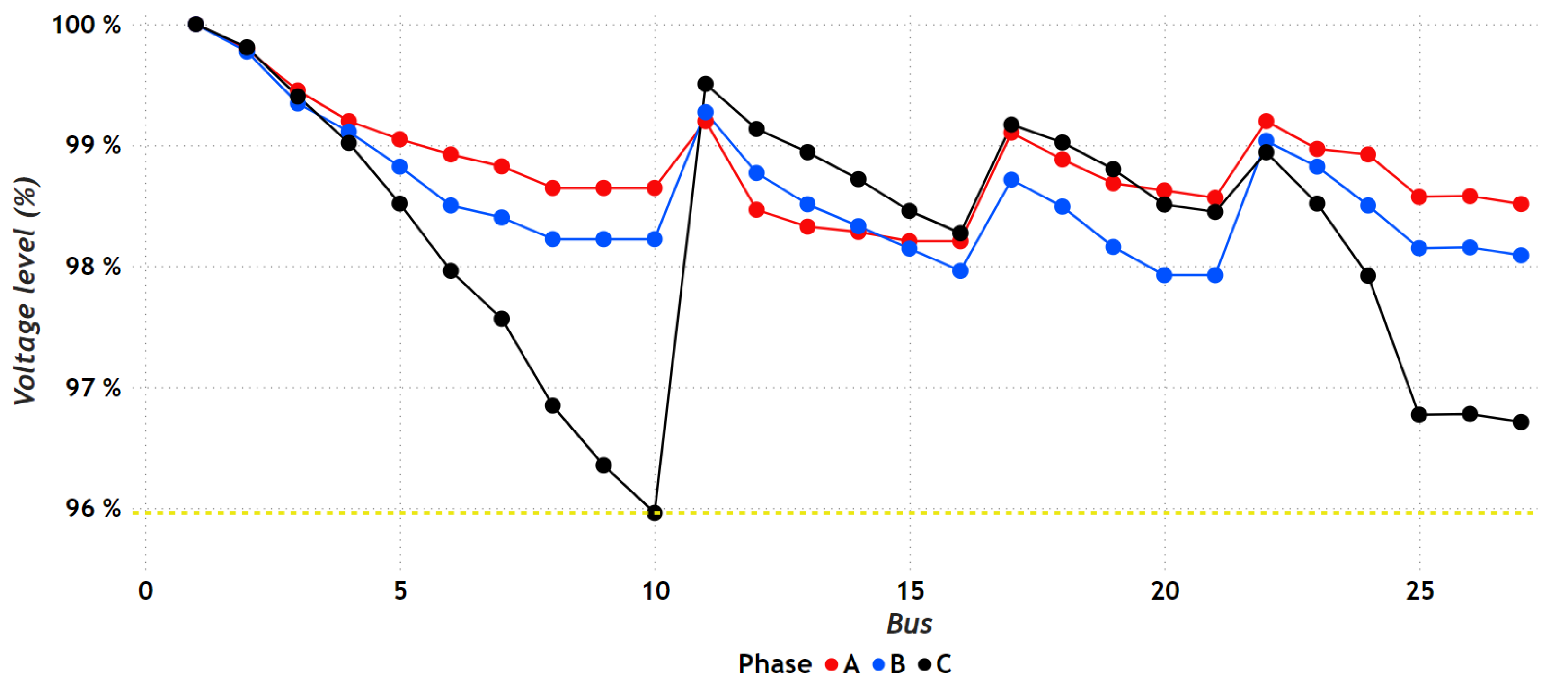
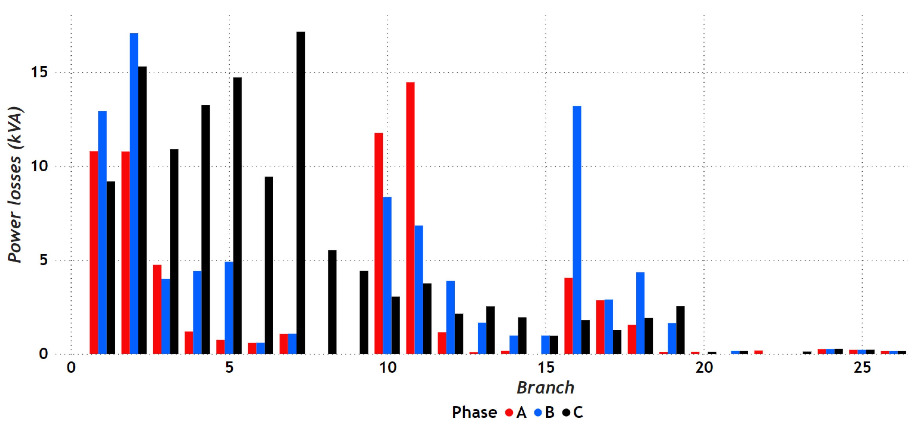
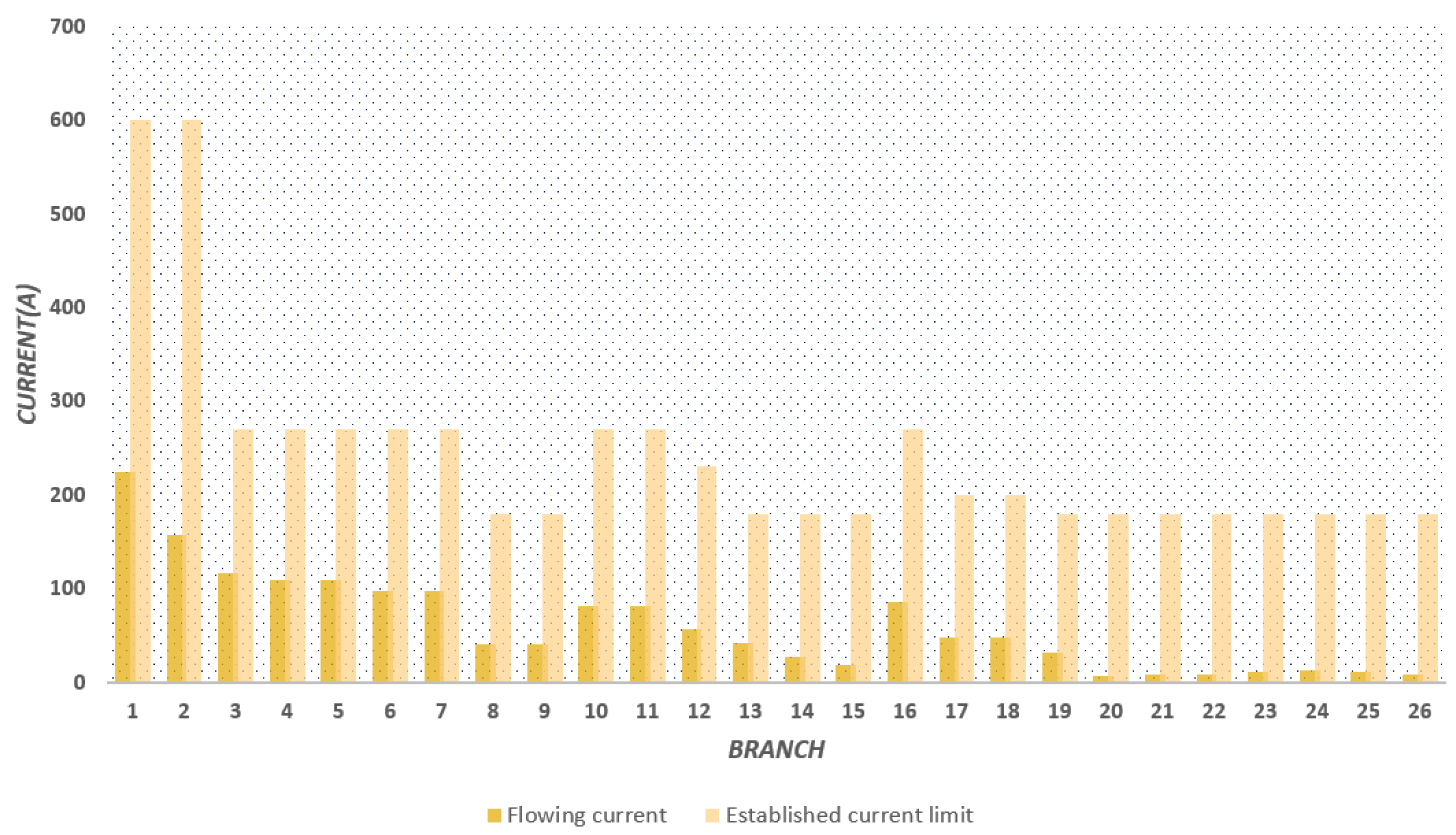
- The levels of loadability shown for each of the lines in the different cases of study guarantee good functioning in the electrical distribution systems tested, additionally ensuring the possibility of future expansions and new load connections.Figure 18. Behavior of the value of the objective function for: () 8-bus system with balanced load; () 27-bus system with balanced load.Figure 18. Behavior of the value of the objective function for: () 8-bus system with balanced load; () 27-bus system with balanced load.
 Figure 19. Behavior of the value of the objective function for: () 8-bus system with unbalanced load; () 27-bus system with unbalanced load.Figure 19. Behavior of the value of the objective function for: () 8-bus system with unbalanced load; () 27-bus system with unbalanced load.


7.4. Selection of Conductors Considering Different Load Periods
- Case 1: The evaluation of the optimization methodology during the peak load condition, condition, i.e., under the same simulation conditions used for the 8- and 27-bus grids.
- Case 2: The evaluation of the optimization methodology considering daily load variations, according to Table 15 data.
- Case 3: The evaluation of the optimization methodology considering three different demand periods over the year as follows: (i) 1000 h at 100 percent demand, (ii) 6760 h at 60 percent demand, (iii) 1000 h at 30 percent demand.Table 15. Daily demand variation for the 33-bus grid.
Time (h) Demand (pu) Time (h) Demand (pu) Time (h) Demand (pu) 1 0.684511335492475 9 0.706039245570585 17 0.874071251666984 2 0.644122690036197 10 0.787007048961707 18 1 3 0.613069156029720 11 0.839016955610593 19 0.983615926843208 4 0.599733282530006 12 0.852733854067441 20 0.936368832158506 5 0.588874071251667 13 0.870642027052772 21 0.887597637645266 6 0.598018670222900 14 0.834254143646409 22 0.809297008954087 7 0.626786054486569 15 0.816536483139646 23 0.745856353591160 8 0.651743189178891 16 0.819394170318156 24 0.733473042484283
- i.
- The investment and operating cost in Case 1, where the peak load condition is analyzed during the year, shows that to minimize the costs of energy losses, the size of the conductors is increased considerably, being this investment costs about of the total costs of the plan. This is an expected result since, as observed in Table 16, the solution of Case 1 has the largest conductor sizes compared with the remainder of the simulation cases.
- ii.
- The operation scenario considering the daily load profile shows the more realistic simulation scenario (see Case 2) where the energy losses considerably reduce their costs when compared to the peak load operation scenario (about ), which has a direct effect on the conductors selected to supply the energy load within this daily operation case. Note that the reduction in the investment costs when compared to Case 1 and Case 2 is about . This is an expected reduction in the investment costs since these are nonlinearly related to the energy loss costs, which implies that smaller conductor sizes can be found as an adequate balance between investment and operating costs.
- iii.
- Case 3 shows an intermediate solution scenario between Cases 1 and 2, with a total investment of USD/year distributed about on investment in conductors and in costs of the energy losses. Note that what happened with Case 1, the expected energy losses costs of the network, have an essential influence on the size of the conductors selected (see Table 16); in addition, note that for the distribution company, the solution in Case 3 can be the most attractive alternative since it has moderate investment costs with the main advantage that the selected conductors can support future load increments without any changes in the grid structure.
- iiii.
- Analyzing the processing times, we obtained that for Case 1 it takes 215.5422075 seconds to converge in a single evaluation, while Case 2 and 3 take 4514.526068 and 488.239934 seconds, respectively. Based on the results obtained we can observe that Cases 1 and 2 don’t represent big computational processing times, in other hand for third case its time increases among other things for daily demand variations.
8. Conclusions and Future Work
Author Contributions
Funding
Institutional Review Board Statement
Informed Consent Statement
Data Availability Statement
Acknowledgments
Conflicts of Interest
References
- Ramírez Castaño, S. Power Distribution Networks; Departamento de Ingeniería Eléctrica, Electrónica y Computación, Universidad Nacional de Colombia: Manizalez, Colombia, 2004; Available online: https://repositorio.unal.edu.co/handle/unal/57581 (accessed on 23 December 2022).
- Denton, W.; Reps, D. Distribution-substation and primary-feeder planning. Electr. Eng. 1955, 74, 804–809. [Google Scholar] [CrossRef]
- Agarwal, U.; Jain, N. Distributed energy resources and supportive methodologies for their optimal planning under modern distribution network: A review. Technol. Econ. Smart Grids Sustain. Energy 2019, 4, 1–21. [Google Scholar] [CrossRef]
- Koziel, S.; Hilber, P.; Westerlund, P.; Shayesteh, E. Investments in data quality: Evaluating impacts of faulty data on asset management in power systems. Appl. Energy 2021, 281, 116057. [Google Scholar] [CrossRef]
- Ahmadian, A.; Elkamel, A.; Mazouz, A. An improved hybrid particle swarm optimization and tabu search algorithm for expansion planning of large dimension electric distribution network. Energies 2019, 12, 3052. [Google Scholar] [CrossRef]
- Kazmi, S.A.A.; Shahzad, M.K.; Khan, A.Z.; Shin, D.R. Smart distribution networks: A review of modern distribution concepts from a planning perspective. Energies 2017, 10, 501. [Google Scholar] [CrossRef]
- Ponnavaikko, M.; Rao, K.P. Optimal distribution system planning. IEEE Trans. Power Appar. Syst. 1981, 6, 2969–2977. [Google Scholar] [CrossRef]
- Ponnavaikko, N.; Rao, K.P.; Venkata, S. Distribution system planning through a quadratic mixed integer programming approach. IEEE Trans. Power Deliv. 1987, 2, 1157–1163. [Google Scholar] [CrossRef]
- Adams, R.; Laughton, M. Optimal planning of power networks using mixed-integer programming. Part 1: Static and time-phased network synthesis. Proc. Inst. Electr. Eng. IET 1974, 121, 139–147. [Google Scholar] [CrossRef]
- Islam, S.J.; Ghani, M.R.A. Economical optimization of conductor selection in planning radial distribution networks. In Proceedings of the 1999 IEEE Transmission and Distribution Conference (Cat. No. 99CH36333), New Orleans, LA, USA, 11–16 April 1999; Volume 2, pp. 858–863. [Google Scholar] [CrossRef]
- Joshi, D.; Burada, S.; Mistry, K.D. Distribution system planning with optimal conductor selection. In Proceedings of the 2017 Recent Developments in Control, Automation & Power Engineering (RDCAPE), Noida, India, 26–27 October 2017; pp. 263–268. [Google Scholar] [CrossRef]
- Falaghi, H.; Ramezani, M.; Haghifam, M.R.; Milani, K.R. Optimal selection of conductors in radial distribution systems with time varying load. In Proceedings of the CIRED 2005-18th International Conference and Exhibition on Electricity Distribution, Turin, Italy, 6–9 June 2005; pp. 1–4. [Google Scholar] [CrossRef]
- Ponnavaikko, M.; Rao, K.P. An approach to optimal distribution system planning through conductor gradation. IEEE Trans. Power Appar. Syst. 1982, 6, 1735–1742. [Google Scholar] [CrossRef]
- Mendoza, F.; Requena, D.; Bemal-Agustin, J.L.; Domínguez-Navarro, J.A. Optimal conductor size selection in radial power distribution systems using evolutionary strategies. In Proceedings of the 2006 IEEE/PES Transmission & Distribution Conference and Exposition: Latin America, Caracas, Venezuela, 15–18 August 2006; pp. 1–5. [Google Scholar] [CrossRef]
- Legha, M.M.; Javaheri, H.; Legha, M.M. Optimal Conductor Selection in Radial Distribution Systems for Productivity Improvement Using Genetic Algorithm. Iraqi J. Electr. Electron. Eng. 2013, 9, 29–35. [Google Scholar] [CrossRef]
- Rao, R.S.; Satish, K.; Narasimham, S. Optimal conductor size selection in distribution systems using the harmony search algorithm with a differential operator. Electr. Power Components Syst. 2011, 40, 41–56. [Google Scholar] [CrossRef]
- Momoh, I.; Jibril, Y.; Jimoh, B.; Abubakar, A.; Ajayi, O.; Abubakar, A.; Sulaiman, S.; Yusuf, S. Effect of an optimal conductor size selection scheme for single wire earth return power distribution networks for rural electrification. ATBU J. Sci. Technol. Educ. 2019, 7, 286–295. [Google Scholar]
- Manikandan, S.; Sasitharan, S.; Rao, J.V.; Moorthy, V. Analysis of optimal conductor selection for radial distribution systems using DPSO. In Proceedings of the 2016 3rd International Conference on Electrical Energy Systems (ICEES), Chennai, India, 17–19 March 2016; pp. 96–101. [Google Scholar] [CrossRef]
- Kalesa, B.M. Conductor selection optimization in radial distribution system considering load growth using MDE algorithm. World J. Model. D Simul. 2014, 10, 175–184. [Google Scholar]
- Abdelaziz, A.Y.; Fathy, A. A novel approach based on crow search algorithm for optimal selection of conductor size in radial distribution networks. Eng. Sci. Technol. Int. J. 2017, 20, 391–402. [Google Scholar] [CrossRef]
- Ismael, S.M.; Aleem, S.H.A.; Abdelaziz, A.Y. Optimal selection of conductors in Egyptian radial distribution systems using sine-cosine optimization algorithm. In Proceedings of the 2017 Nineteenth International Middle East Power Systems Conference (MEPCON), Cairo, Egypt, 19–21 December 2017; pp. 103–107. [Google Scholar] [CrossRef]
- Ismael, S.M.; Aleem, S.H.A.; Abdelaziz, A.Y.; Zobaa, A.F. Practical considerations for optimal conductor reinforcement and hosting capacity enhancement in radial distribution systems. IEEE Access 2018, 6, 27268–27277. [Google Scholar] [CrossRef]
- Kumari, M.; Singh, V.; Ranjan, R. Optimal selection of conductor in RDS considering weather condition. In Proceedings of the 2018 International Conference on Computing, Power and Communication Technologies (GUCON), Greater Noida, India, 28–29 September 2018; pp. 647–651. [Google Scholar] [CrossRef]
- Ismael, S.M.; Aleem, S.; Abdelaziz, A.Y. Optimal conductor selection in radial distribution systems using whale optimization algorithm. J. Eng. Sci. Technol. 2019, 14, 87–107. [Google Scholar]
- Ramana, T.; Nararaju, K.; Ganesh, V.; Sivanagaraju, S. Customer Loss Allocation Reduction Using Optimal Conductor Selection in Electrical Distribution System. In Emerging Trends in Electrical, Communications, and Information Technologies; Springer: Berlin/Heildeberg, Germany, 2020; pp. 369–379. [Google Scholar] [CrossRef]
- Martínez-Gil, J.F.; Moyano-García, N.A.; Montoya, O.D.; Alarcon-Villamil, J.A. Optimal Selection of Conductors in Three-Phase Distribution Networks Using a Discrete Version of the Vortex Search Algorithm. Computation 2021, 9, 80. [Google Scholar] [CrossRef]
- Thenepalle, M. A comparative study on optimal conductor selection for radial distribution network using conventional and genetic algorithm approach. Int. J. Comput. Appl. 2011, 17, 6–13. [Google Scholar] [CrossRef]
- Samal, P.; Mohanty, S.; Ganguly, S. Simultaneous capacitor allocation and conductor sizing in unbalanced radial distribution systems using differential evolution algorithm. In Proceedings of the 2016 National Power Systems Conference (NPSC), Bhubaneswar, India, 19–21 December 2016; pp. 1–6. [Google Scholar] [CrossRef]
- Abul’Wafa, A.R. Multi-conductor feeder design for radial distribution networks. Electr. Power Syst. Res. 2016, 140, 184–192. [Google Scholar] [CrossRef]
- Nivia Torres, D.J.; Salazar Alarcón, G.A.; Montoya, O.D. Selección óptima de conductores en redes de distribución trifásicas utilizando el algoritmo metaheurístico de Newton. Ingeniería 2022, 27, e19303. [Google Scholar] [CrossRef]
- Montoya, O.D. Notes on the Dimension of the Solution Space in Typical Electrical Engineering Optimization Problems. Ingeniería 2022, 27, e19310. [Google Scholar] [CrossRef]
- Zhang, Y.; Jin, Z.; Mirjalili, S. Generalized normal distribution optimization and its applications in parameter extraction of photovoltaic models. Energy Convers. Manag. 2020, 224, 113301. [Google Scholar] [CrossRef]
- Cortés-Caicedo, B.; Avellaneda-Gómez, L.S.; Montoya, O.D.; Alvarado-Barrios, L.; Chamorro, H.R. Application of the Vortex Search Algorithm to the Phase-Balancing Problem in Distribution Systems. Energies 2021, 14, 1282. [Google Scholar] [CrossRef]
- Abdel-Basset, M.; Mohamed, R.; Abouhawwash, M.; Chang, V.; Askar, S. A local search-based generalized normal distribution algorithm for permutation flow shop scheduling. Appl. Sci. 2021, 11, 4837. [Google Scholar] [CrossRef]
- Wang, C.; Liu, P.; Zhang, T.; Sun, J. The adaptive vortex search algorithm of optimal path planning for forest fire rescue UAV. In Proceedings of the 2018 IEEE 3rd Advanced Information Technology, Electronic and Automation Control Conference (IAEAC), Chongqing, China, 12–14 October 2018; pp. 400–403. [Google Scholar] [CrossRef]
- Doğan, B. A modified vortex search algorithm for numerical function optimization. arXiv 2016, arXiv:1606.02710. [Google Scholar] [CrossRef]


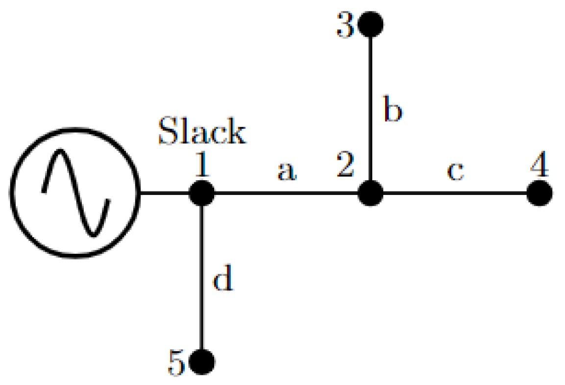
| Nomenclature of Branch | From Bus | To Bus |
|---|---|---|
| a | 1 | 2 |
| b | 2 | 3 |
| c | 2 | 4 |
| d | 1 | 5 |
| Parameter | Value | Unit |
|---|---|---|
| Energy cost | 0.1390 | (US$/kWh) |
| Iterations | 1000 | - |
| Population size | 30 | - |
| Tolerance | - |
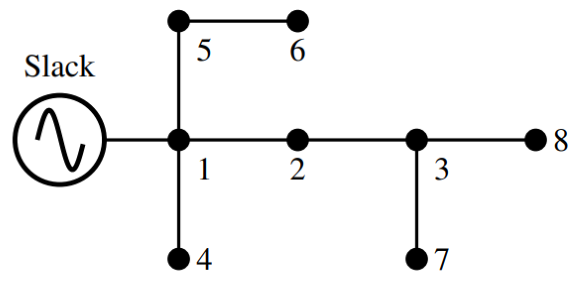
| Line | Bus | Bus | (km) | (kW) | (kvar) |
|---|---|---|---|---|---|
| 1 | 1 | 2 | 1.00 | 1054.2 | 0 |
| 2 | 2 | 3 | 1.00 | 806.5 | 0 |
| 3 | 1 | 4 | 1.00 | 2632.5 | 0 |
| 4 | 1 | 5 | 1.00 | 609 | 0 |
| 5 | 5 | 6 | 1.00 | 2034.5 | 0 |
| 6 | 3 | 7 | 1.00 | 932.8 | 0 |
| 7 | 3 | 8 | 1.00 | 1731.4 | 0 |
| Bus | (kW) | (kvar) | (kW) | (kvar) | (kW) | (kvar) |
|---|---|---|---|---|---|---|
| 2 | 3162.6 | 0 | 0 | 0 | 0 | 0 |
| 3 | 0 | 0 | 2419.5 | 0 | 0 | 0 |
| 4 | 0 | 0 | 0 | 0 | 7897.5 | 0 |
| 5 | 913.5 | 0 | 913.5 | 0 | 0 | 0 |
| 6 | 0 | 0 | 3051.6 | 0 | 3051.6 | 0 |
| 7 | 2798.4 | 0 | 0 | 0 | 0 | 0 |
| 8 | 1298.55 | 0 | 2597.1 | 0 | 1298.55 | 0 |
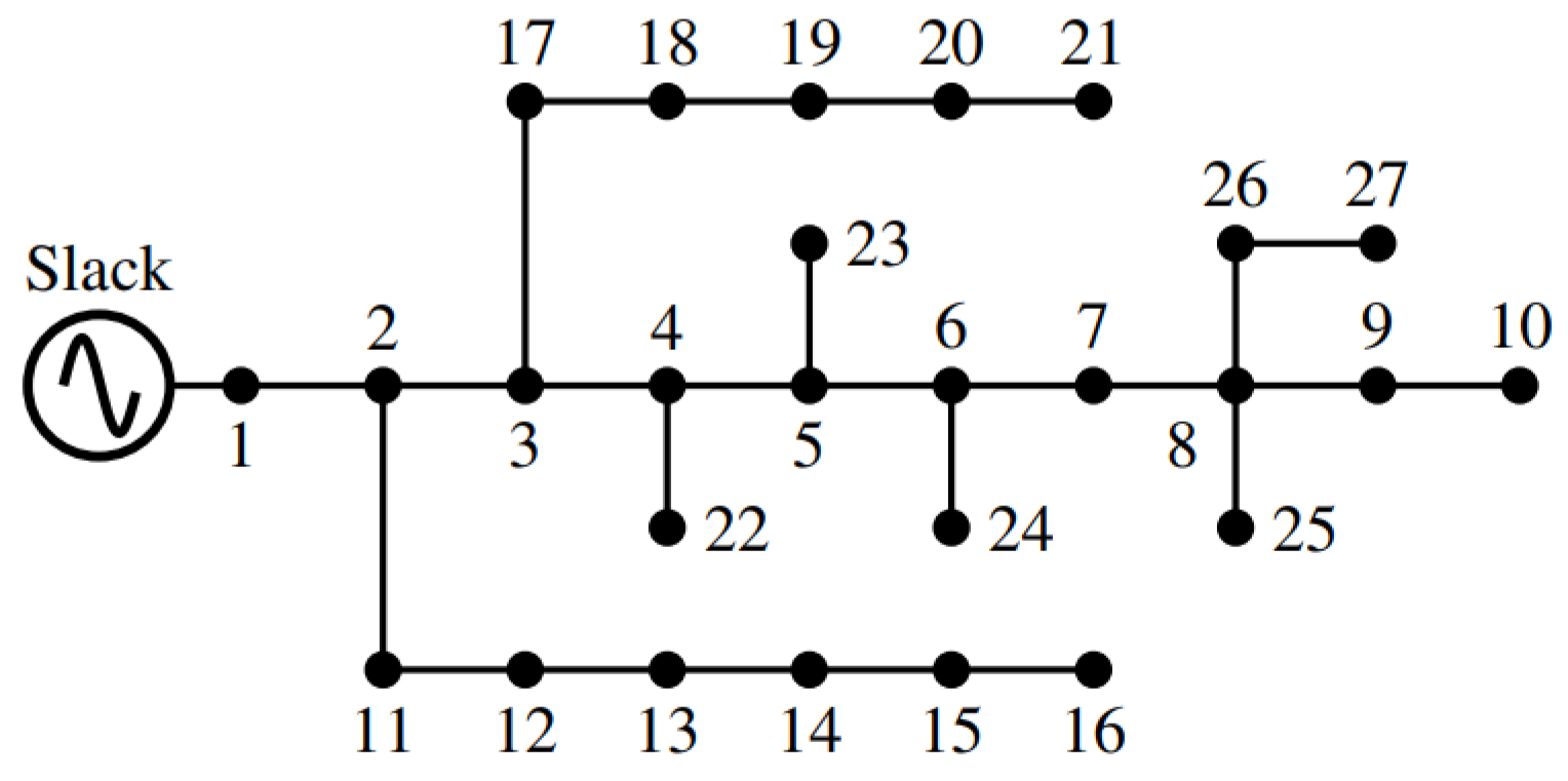
| Line | Bus | Bus | (km) | (kW) | (kvar) |
|---|---|---|---|---|---|
| 1 | 1 | 2 | 0.55 | 0 | 0 |
| 2 | 2 | 3 | 1.50 | 0 | 0 |
| 3 | 3 | 4 | 0.45 | 297.5 | 184.4 |
| 4 | 4 | 5 | 0.63 | 0 | 0 |
| 5 | 5 | 6 | 0.70 | 255 | 158 |
| 6 | 6 | 7 | 0.55 | 0 | 0 |
| 7 | 7 | 8 | 1.00 | 212.5 | 131.7 |
| 8 | 8 | 9 | 1.25 | 0 | 0 |
| 9 | 9 | 10 | 1.00 | 266.1 | 164.9 |
| 10 | 2 | 11 | 1.00 | 85 | 52.7 |
| 11 | 11 | 12 | 1.23 | 340 | 210.7 |
| 12 | 12 | 13 | 0.75 | 297.5 | 184.4 |
| 13 | 13 | 14 | 0.56 | 191.3 | 118.5 |
| 14 | 14 | 15 | 1.00 | 106.3 | 65.8 |
| 15 | 15 | 16 | 1.00 | 255 | 158 |
| 16 | 3 | 17 | 1.00 | 255 | 158 |
| 17 | 17 | 18 | 0.60 | 127.5 | 79 |
| 18 | 18 | 19 | 0.90 | 297.5 | 184.4 |
| 19 | 19 | 20 | 0.95 | 340 | 210.7 |
| 20 | 20 | 21 | 1.00 | 85 | 52.7 |
| 21 | 4 | 22 | 1.00 | 106.3 | 65.8 |
| 22 | 5 | 23 | 1.00 | 55.3 | 34.2 |
| 23 | 6 | 24 | 0.40 | 69.7 | 43.2 |
| 24 | 8 | 25 | 0.60 | 255 | 158 |
| 25 | 8 | 26 | 0.60 | 63.8 | 39.5 |
| 26 | 26 | 27 | 0.80 | 170 | 105.4 |
| Bus | (kW) | (kvar) | (kW) | (kvar) | (kW) | (kvar) |
|---|---|---|---|---|---|---|
| 2 | 0 | 0 | 0 | 0 | 0 | 0 |
| 3 | 0 | 0 | 0 | 0 | 0 | 0 |
| 4 | 892.5 | 553.2 | 0 | 0 | 0 | 0 |
| 5 | 0 | 0 | 0 | 0 | 0 | 0 |
| 6 | 0 | 0 | 765 | 474 | 0 | 0 |
| 7 | 0 | 0 | 0 | 0 | 0 | 0 |
| 8 | 0 | 0 | 0 | 0 | 637.5 | 395.1 |
| 9 | 0 | 0 | 0 | 0 | 0 | 0 |
| 10 | 0 | 0 | 0 | 0 | 798.3 | 494.7 |
| 11 | 0 | 0 | 255 | 158.1 | 0 | 0 |
| 12 | 1020 | 632.1 | 0 | 0 | 0 | 0 |
| 13 | 446.25 | 276.6 | 446.25 | 276.6 | 0 | 0 |
| 14 | 0 | 0 | 286.95 | 177.75 | 286.95 | 177.75 |
| 15 | 159.45 | 98.7 | 0 | 0 | 159.45 | 98.7 |
| 16 | 0 | 0 | 382.5 | 237 | 382.5 | 237 |
| 17 | 1 | 0 | 765 | 474 | 0 | 0 |
| 18 | 382.5 | 237 | 0 | 0 | 0 | 0 |
| 19 | 446.25 | 276.6 | 446.25 | 276.6 | 0 | 0 |
| 20 | 0 | 0 | 510 | 316.05 | 510 | 316.05 |
| 21 | 127.5 | 79.05 | 0 | 0 | 127.5 | 79.05 |
| 22 | 0 | 0 | 159.75 | 98.7 | 159.75 | 98.7 |
| 23 | 165.9 | 102.6 | 0 | 0 | 0 | 0 |
| 24 | 0 | 0 | 0 | 0 | 209.1 | 129.6 |
| 25 | 255 | 158 | 255 | 158 | 255 | 158 |
| 26 | 63.8 | 39.5 | 63.8 | 39.5 | 63.8 | 39.5 |
| 27 | 170 | 105.4 | 170 | 105.4 | 170 | 105.4 |
| Gauge (c) | () | () | (A) | (US$/km) |
|---|---|---|---|---|
| 1 | 0.8763 | 0.4133 | 180 | 1986 |
| 2 | 0.6960 | 0.4133 | 200 | 2790 |
| 3 | 0.5518 | 0.4077 | 230 | 3815 |
| 4 | 0.4387 | 0.3983 | 270 | 5090 |
| 5 | 0.3480 | 0.3899 | 300 | 8067 |
| 6 | 0.2765 | 0.3610 | 340 | 12,673 |
| 7 | 0.0966 | 0.1201 | 600 | 23,419 |
| 8 | 0.0853 | 0.0950 | 720 | 30,070 |
| Method | Gauges | Investment in Conductors (US$) | Losses (US$) | Annual Costs (US$) |
|---|---|---|---|---|
| TGA | {6,5,3,4,4,1,4} | 125,433 | 406,222.461 | 531,655.461 |
| CBGA | {6,6,4,4,4,1,4} | 143,076 | 373,155.965 | 516,231.965 |
| GAMS | {6,4,4,5,4,1,2} | 122,358 | 416,681.580 | 539,039.580 |
| TBA | {6,5,4,4,4,1,3} | 125,433 | 397,754.442 | 523,187.442 |
| VSA | {6,6,5,5,4,2,4} | 163,350 | 345,007.959 | 508,357.959 |
| NMA | {6,6,5,5,4,2,4} | 163,350 | 345,007.959 | 508,357.959 |
| GNDO | {7,7,5,5,4,2,4} | 227.826 | 228,143.791 | 455,969.791 |
| Method | Gauges | Investment in Conductors (US$) | Losses (US$) | Annual Costs (US$) |
|---|---|---|---|---|
| VSA | {7,7,5,4,4,3,3,1,1,4,4,2,3 2,1,4,4,2,2,2,1,1,2,2,1,1} | 344,352.150 | 217,672.327 | 562,024.477 |
| NMA | {7,7,4,4,4,4,3,1,1,4,4,3,3 1,2,4,3,2,1,1,1,1,2,2,1,1} | 337,744.800 | 219,950.455 | 557,695.255 |
| GNDO | {7,7,4,4,4,3,3,1,1,4,4,2,1 1,1,3,2,2,1,1,1,1,1,1,1,1} | 319,768.08 | 230,115.492 | 549,883.572 |
| Method | Gauges | Investment in Conductors (US$) | Losses (US$) | Annual Costs (US$) |
|---|---|---|---|---|
| VSA | {7,7,7,5,5,4,4} | 289,713 | 269,045.394 | 558,758.394 |
| NMA | {7,7,7,5,5,4,4} | 289,713 | 269,045.394 | 558,758.394 |
| GNDO | {7,7,7,5,5,4,4} | 289,713 | 269,045.394 | 558,758.394 |
| Method | Gauges | Investment in Conductors (US$) | Losses (US$) | Annual Costs (US$) |
|---|---|---|---|---|
| VSA | {7,7,5,4,4,4,4,2,2,4,4,3,2 1,1,2,3,2,1,2,2,1,2,2,4,1} | 350,392.95 | 257,999.185 | 608,392.135 |
| NMA | {7,7,4,4,4,3,4,2,1,4,4,4,2 1,1,4,3,2,2,1,1,1,2,2,2,1} | 344,954.40 | 252,624.608 | 597,579.008 |
| GNDO | {7,7,4,4,4,4,4,1,1,4,4,3,1 1,1,4,2,2,1,1,1,1,1,1,1,1} | 331,828.08 | 257,190.720 | 589,018.800 |
| Line | Bus | Bus | (km) |
|---|---|---|---|
| 1 | 1 | 2 | 0.0699 |
| 2 | 2 | 3 | 0.3720 |
| 3 | 3 | 4 | 0.2762 |
| 4 | 4 | 5 | 0.2876 |
| 5 | 5 | 6 | 0.7630 |
| 6 | 6 | 7 | 0.4030 |
| 7 | 7 | 8 | 1.4733 |
| 8 | 8 | 9 | 0.8850 |
| 9 | 9 | 10 | 0.8900 |
| 10 | 10 | 11 | 0.1308 |
| 11 | 11 | 12 | 0.2491 |
| 12 | 12 | 13 | 1.3115 |
| 13 | 13 | 14 | 0.6272 |
| 14 | 14 | 15 | 0.5585 |
| 15 | 15 | 16 | 0.6457 |
| 16 | 16 | 17 | 1.5050 |
| 17 | 17 | 18 | 0.6530 |
| 18 | 2 | 19 | 0.1603 |
| 19 | 19 | 20 | 1.4298 |
| 20 | 20 | 21 | 0.4439 |
| 21 | 21 | 22 | 0.8231 |
| 22 | 3 | 23 | 0.3798 |
| 23 | 23 | 24 | 0.8035 |
| 24 | 24 | 25 | 0.7985 |
| 25 | 6 | 26 | 0.1532 |
| 26 | 26 | 27 | 0.2145 |
| 27 | 27 | 28 | 0.9963 |
| 28 | 28 | 29 | 0.7524 |
| 29 | 29 | 30 | 0.3830 |
| 30 | 30 | 31 | 0.9687 |
| 31 | 31 | 32 | 0.3362 |
| 32 | 32 | 33 | 0.4356 |
| Bus | (kW) | (kvar) | (kW) | (kvar) | (kW) | (kvar) |
|---|---|---|---|---|---|---|
| 2 | 100 | 50 | 100 | 60 | 0 | 0 |
| 3 | 90 | 0 | 90 | 40 | 0 | 0 |
| 4 | 120 | 75 | 120 | 80 | 150 | 90 |
| 5 | 60 | 20 | 60 | 30 | 60 | 30 |
| 6 | 60 | 18 | 60 | 20 | 60 | 20 |
| 7 | 200 | 150 | 0 | 0 | 100 | 100 |
| 8 | 200 | 0 | 200 | 100 | 0 | 0 |
| 9 | 60 | 60 | 0 | 0 | 0 | 0 |
| 10 | 60 | 60 | 60 | 20 | 0 | 0 |
| 11 | 45 | 30 | 45 | 30 | 45 | 30 |
| 12 | 0 | 0 | 60 | 35 | 155 | 100 |
| 13 | 60 | 110 | 60 | 35 | 60 | 35 |
| 14 | 120 | 80 | 190 | 80 | 120 | 80 |
| 15 | 60 | 10 | 60 | 50 | 60 | 10 |
| 16 | 60 | 20 | 110 | 80 | 60 | 20 |
| 17 | 60 | 20 | 150 | 95 | 0 | 0 |
| 18 | 90 | 40 | 100 | 0 | 90 | 40 |
| 19 | 0 | 0 | 0 | 0 | 90 | 40 |
| 20 | 210 | 50 | 85 | 40 | 70 | 75 |
| 21 | 90 | 40 | 110 | 40 | 110 | 20 |
| 22 | 300 | 400 | 0 | 0 | 90 | 40 |
| 23 | 90 | 50 | 70 | 0 | 0 | 0 |
| 24 | 420 | 200 | 420 | 200 | 420 | 200 |
| 25 | 120 | 75 | 0 | 0 | 150 | 100 |
| 26 | 60 | 25 | 80 | 25 | 0 | 0 |
| 27 | 0 | 0 | 80 | 25 | 0 | 0 |
| 28 | 60 | 20 | 48 | 24 | 60 | 20 |
| 29 | 120 | 70 | 185 | 75 | 120 | 70 |
| 30 | 200 | 600 | 400 | 400 | 500 | 600 |
| 31 | 150 | 70 | 120 | 90 | 150 | 70 |
| 32 | 210 | 100 | 120 | 35 | 210 | 100 |
| 33 | 60 | 40 | 100 | 750 | 0 | 0 |
| Line | Case 1 | Case 2 | Case 3 |
|---|---|---|---|
| 1 | 7 | 4 | 7 |
| 2 | 7 | 4 | 7 |
| 3 | 7 | 4 | 7 |
| 4 | 7 | 4 | 7 |
| 5 | 7 | 4 | 7 |
| 6 | 7 | 4 | 7 |
| 7 | 7 | 4 | 7 |
| 8 | 7 | 4 | 7 |
| 9 | 7 | 4 | 7 |
| 10 | 7 | 4 | 7 |
| 11 | 7 | 3 | 6 |
| 12 | 7 | 3 | 6 |
| 13 | 7 | 3 | 4 |
| 14 | 6 | 2 | 4 |
| 15 | 5 | 1 | 1 |
| 16 | 5 | 1 | 1 |
| 17 | 1 | 1 | 1 |
| 18 | 4 | 1 | 5 |
| 19 | 4 | 1 | 2 |
| 20 | 4 | 1 | 1 |
| 21 | 1 | 1 | 1 |
| 22 | 5 | 3 | 4 |
| 23 | 5 | 3 | 4 |
| 24 | 1 | 1 | 1 |
| 25 | 7 | 4 | 7 |
| 26 | 7 | 4 | 5 |
| 27 | 6 | 1 | 5 |
| 28 | 6 | 1 | 3 |
| 29 | 6 | 1 | 3 |
| 30 | 3 | 1 | 1 |
| 31 | 2 | 1 | 1 |
| 32 | 2 | 1 | 1 |
| Case | (USD) | (USD) | Z (USD) |
|---|---|---|---|
| 1 | 814,647.151 | 88,991.787 | 903,638.938 |
| 2 | 195,187.456 | 7246.061 | 202,433.517 |
| 3 | 593,777.672 | 48,350.741 | 642,128.413 |
Disclaimer/Publisher’s Note: The statements, opinions and data contained in all publications are solely those of the individual author(s) and contributor(s) and not of MDPI and/or the editor(s). MDPI and/or the editor(s) disclaim responsibility for any injury to people or property resulting from any ideas, methods, instructions or products referred to in the content. |
© 2023 by the authors. Licensee MDPI, Basel, Switzerland. This article is an open access article distributed under the terms and conditions of the Creative Commons Attribution (CC BY) license (https://creativecommons.org/licenses/by/4.0/).
Share and Cite
Vega-Forero, J.A.; Ramos-Castellanos, J.S.; Montoya, O.D. Application of the Generalized Normal Distribution Optimization Algorithm to the Optimal Selection of Conductors in Three-Phase Asymmetric Distribution Networks. Energies 2023, 16, 1311. https://doi.org/10.3390/en16031311
Vega-Forero JA, Ramos-Castellanos JS, Montoya OD. Application of the Generalized Normal Distribution Optimization Algorithm to the Optimal Selection of Conductors in Three-Phase Asymmetric Distribution Networks. Energies. 2023; 16(3):1311. https://doi.org/10.3390/en16031311
Chicago/Turabian StyleVega-Forero, Julián Alejandro, Jairo Stiven Ramos-Castellanos, and Oscar Danilo Montoya. 2023. "Application of the Generalized Normal Distribution Optimization Algorithm to the Optimal Selection of Conductors in Three-Phase Asymmetric Distribution Networks" Energies 16, no. 3: 1311. https://doi.org/10.3390/en16031311
APA StyleVega-Forero, J. A., Ramos-Castellanos, J. S., & Montoya, O. D. (2023). Application of the Generalized Normal Distribution Optimization Algorithm to the Optimal Selection of Conductors in Three-Phase Asymmetric Distribution Networks. Energies, 16(3), 1311. https://doi.org/10.3390/en16031311