Abstract
Production forecasting using numerical simulation has become a standard in the oil and gas industry. The model construction process requires an explicit definition of multiple uncertain parameters; thus, the outcome of the modelling is also uncertain. For the reservoirs with production data, the uncertainty can be reduced by history-matching. However, the manual matching procedure is time-consuming and usually generates one deterministic realization. Due to the ill-posed nature of the calibration process, the uncertainty cannot be captured sufficiently with only one simulation model. In this paper, the uncertainty quantification process carried out for a gas-condensate reservoir is described. The ensemble-based uncertainty approach was used with the ES-MDA algorithm, conditioning the models to the observed data. Along with the results, the author described the solutions proposed to improve the algorithm’s efficiency and to analyze the factors controlling modelling uncertainty. As a part of the calibration process, various geological hypotheses regarding the presence of an active aquifer were verified, leading to important observations about the drive mechanism of the analyzed reservoir.
1. Introduction
The purpose of using numerical models is to generate forecasts and optimize production from hydrocarbon reservoirs [1]. The importance of reliable production prognoses is driven by their influence on reservoir management decisions [2], which typically represent multi-million dollar expenses. From a practical point of view, the reservoir simulation consists of a numerical solution of nonlinear differential equations in a grid of cells with variable rock and fluid properties [3]. The majority of parameters used in the models are subject to uncertainty, therefore, the modelling outcome is also uncertain [4,5,6]. This problem has been known by the academic community and industry for decades, and still motivates researchers to further work.
For the reservoirs with production data, modeling uncertainty can be reduced by history-matching. The matching process lies in the fine-tuning of input parameters. Typically, this is performed manually until the mismatch between the model response and the observed data is reduced to an acceptable level [2]. Usually, this approach is time-consuming and generates one calibrated realization [4,7]. Due to the ill-posed nature of the calibration process, the uncertainty cannot be captured sufficiently with only one model [8]. In that case, the obvious method for assessing the uncertainty would be to history-match multiple simulation models, generated based on poorly known input parameters [9]. For years this approach was not feasible due to the high computing power cost. However, thanks to IT development and cost reduction initiatives, ensemble-based methods have been adopted for history-matching and uncertainty quantification problems. In this study, a modern data assimilation algorithm was used to analyze a gas-condensate reservoir. For this application, the standard workflow was upgraded by the authors with solutions that improved the algorithm’s efficiency and enabled better interpretation of the modelling results.
1.1. State-of-the-Art Solutions
Among recently published papers covering the uncertainty quantification topic, considerable attention is focused on the data assimilation algorithms, e.g., Ensemble Kalman Filter (EnKF), Ensemble Smoother (ES) or Ensemble Smoother With Multiple Data Assimilation (ES-MDA) [10,11,12]. Mentioned solutions originate from the Kalman filter theory and belong to a class of particle methods where the model of the system is characterized by probability distribution functions (pdfs) of selected parameters [13,14]. In history-matching applications, those algorithms use the pdfs represented by the ensemble of models. At each assimilation step, the algorithm analyses the impact of a specific parameter on the ensemble’s history match quality and proposes an update. The purpose of the update is to condition the entire set of models to the observed data. At the final step, the ensemble of alternative, equally likely and calibrated models can be used to quantify the modelling uncertainty [15].
In this study, the ES-MDA was used to quantify the modelling uncertainty of a gas-condensate reservoir. This method was introduced by Emerick and Reynolds [11] as a complementary solution to the ES. The ES eliminates the need for the recurrent simulation model restarts required in the EnKF. However, in many applications, it has problems with the satisfactory calibration of models due to resolute parameter updates [11]. To overcome the aforementioned drawback, the ES-MDA was introduced. The improvement with this solution was achieved through multiple data assimilations with gentler adjustments. This effect controls the inflated measurement error covariance matrix [10]. Greater history-matching quality leads to better characterization of the uncertainty in the ensemble and future predictions.
The ES-MDA follows the below steps [11,16]:
- Initialization: to generate the initial ensemble of models by sampling the ranges of predefined history-matching parameters and to store the properties of the models in the vector , to determine the number of assimilation steps , the ensemble size and the inflation coefficients consistent with Equation (1).
- 2.
- For to :
- (a)
- Forecast step: run simulation models over a historical period to generate the vector of predicted datawhere g(m) reflects the observation from the simulation model, generated using parameters captured by vector .
- (b)
- Perturbation of observed data vector:where is the historical data vector, is the measurement error matrix with standard deviations of measurement uncertainties at diagonal, and represents an identity matrix with randomly picked numbers from normal distribution on diagonal.
- (c)
- Analysis step: update the vector of parameters for a new set of simulation modelswhere represent the covariance matrices calculated using the following data vectors .
The perturbation step from the above workflow incorporates the inaccuracies of historical data into the calibration process. From a practical point of view, higher perturbations mean less confidence in the measurements and greater trust in the estimates from the simulation models [17]. The consequence of the above statement is that with higher uncertainty around the observed data, the ES-MDA delivers more gentle updates through the assimilation steps. The ES-MDA originates from the Kalman filter concept. In this solution for the linear cases, the weight given to the measurements error and estimates error controls parameter K, called the Kalman gain. In Equation (4), the role of the Kalman gain represents the fraction with covariance matrices in the denominator. The mentioned fraction acts similarly to the Kalman gain, where a low value gives smoother updates, while a high value gives more confidence in the models, leading to stronger parameter updates [18].
1.2. Observed Limitations
The literature review revealed the following areas of improvement for the history-matching and uncertainty quantification workflows conducted by the ES-MDA:
Initial ensemble sampling: as indicated by various researchers, the sampling of the initial ensemble is crucial for the successful application of the data assimilation algorithms in history-matching problems [14,16,19,20]. The selection of parameters should generate an ensemble with optimistic and pessimistic realizations [14], giving the algorithm representative solution space to properly analyze results and propose parameter updates, eliminating the subjective bias introduced by manual tuning of the initial input parameters.
History-matching outcome analysis: the ensemble calibration process is considered a nonlinear and multidimensional problem [11,12]. An analysis of a particular parameter’s impact on the history-matching quality and modelling uncertainty is not straightforward. As a consequence of the above, there is a need for a solution that enables tracking of the modifications introduced by the algorithm during the calibration process, and highlights the most important uncertainties associated with the analyzed reservoir.
2. Case Study
2.1. Subject of Analysis
The ensemble-based history-matching process presented in this paper was carried out for a real gas-condensate reservoir. The hydrocarbons in this field are present in two formations separated by a thick, impermeable shale layer. Table 1 summarizes the average petrophysical properties of the hydrocarbon saturated intervals.

Table 1.
The summary of basic petrophysical properties of the analyzed reservoir.
The gas–water contact was estimated based on the pressure data from the exploration and appraisal wells. The development was conducted with three vertical gas producers equipped with permanently installed downhole pressure gauges. Due to a limited number of reservoir simulator licenses, only the first five years of production data were used in this study. Figure 1 shows the water saturation distribution within the simulation model.
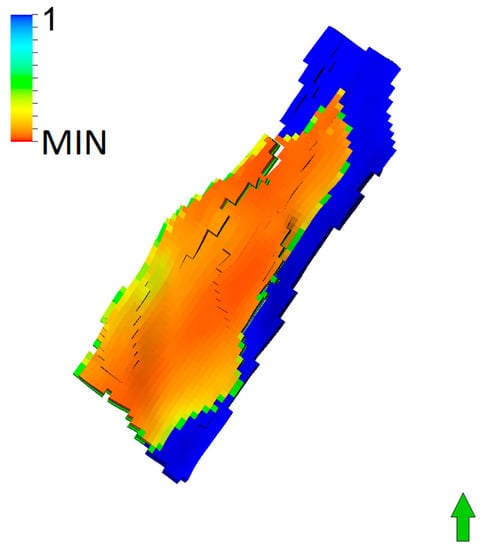
Figure 1.
The distribution of water saturation in the simulation model. Source: PGNiG Upstream Norway AS.
2.2. Description of the Simulation Model and History-Matching Parameterization
Due to the size of the analyzed field, its numerical model uses a black-oil Pressure Volume Temperature (PVT) model. This choice was dictated by the optimization of the computing time [21], therefore the model was created in Eclipse reservoir simulator from Schlumberger. The history-matching process controlled by the ES-MDA was carried out by modification of the following properties, e.g., pore volume, permeability and transmissibility of the faults. Figure 2 illustrates twenty-three areas and eight faults where the ES-MDA introduced the amendments. The main objective of the history-matching was to replicate the historical shut-in bottom-hole pressures recorded in the gas producers over one and two years of production. The remaining production data was used as a validation set to check the history match quality and mapped uncertainties. Due to the lack of formation water production, there was no need to calibrate water rates. Calibration of the gas–oil ratio was unnecessary as the PVT model provided reliable condensate rates as long as the model matched pressures and gas rates.
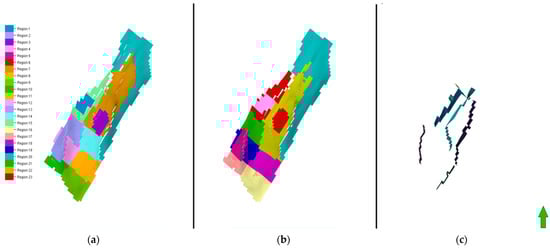
Figure 2.
The regions where the ES-MDA introduced updates during the history-matching process. (a) Shallower formation; (b) deeper formation; (c) faults. Source: PGNiG Upstream Norway AS.
The regions from Figure 2 were proposed based on the experience from other history-matching exercises conducted for the neighboring fields. Regions 1, 2, 3, 11, 12 and 13 are penetrated by the gas producers, whereas the remaining regions cover areas in between the wells. The above split enabled good control over near-wellbore and boundary effects responsible for model calibration. The ranges of uncertain parameters used in the calibration process have been established based on the geological documentation prepared before the production start-up.
The list of all parameters with respective multipliers is summarized in Table 2. For hydrocarbon-saturated regions, the permeability could vary from −50% up to +20%, whereas the pore volume could change by ±30%. A wider multiplier range is assumed for region 20, to reflect higher uncertainty around the size and hydrodynamic properties of the water-bearing sandstones. The transmissibility for all faults could change from closed (multiplier = 0) to fully open (multiplier = 1). The outcome of the first history-matching attempt, performed using data from Table 2, is further described in the text as a mixed scenario. In this case, the ES-MDA could decide whether the aquifer is activated or deactivated during the conditioning process.
Table 2.
The ranges of uncertain parameters used by the ES-MDA during the history-matching.
In order to verify the solutions provided by the ES-MDA, it was decided to perform additional history-matching runs after the first conditioning. Further modelling included two explicitly defined aquifer scenarios. The first assumed no active aquifer, while the second always had an active aquifer with variable strength. The above scenarios were modelled by the parameters set out in Table 3. The aquifer’s permeability and pore volume are controlled by multipliers in region 20, whereas 4, 5 and 6 faults act as barriers limiting water drive. Other parameters remained unchanged compared to the values used for the mixed scenario.
Table 3.
The list of parameters used for aquifer scenario modelling.
2.3. ES-MDA Settings
The uncertainty related to the observed data has also been included in the ES-MDA workflow. For the analyzed field, the historical data uncertainty concerns the shut-in bottom-hole pressures. The downhole pressure gauges in the production wells are installed shallower than the top of the reservoir section. This well design enables the accumulation of liquids below the gauge during the shut-in periods, leading to potential underestimation of the reservoir pressure. The measurement uncertainty of the pressure gauge is defined by the manufacturer at the level of ± 1 bar. This, together with the mentioned liquid problem, allowed the author to propose the following shut-in bottom-hole pressure uncertainties listed in Table 4.
Table 4.
The shut-in bottom hole pressures uncertainty for production wells.
The inflation coefficients and the number of assimilation steps were set as proposed by Emerick and Reynolds [21]: α1 = 9.33, α2 = 7, α3 = 4, α4 = 2. In addition, the author added a fifth assimilation step in the workflow, which does not include the observed data perturbation step during the data assimilation process. The purpose of that was to check the impact of the observed data uncertainty on the history match quality and mapped uncertainties.
Taking into account the complexity of the conducted calibration exercise and the examples of other assisted history-matching cases available in the literature, the author arbitrarily assumed that every ensemble consists of forty simulation models.
After the history-matching, the models were switched to the prediction mode. During the first five years, the production was controlled by historically measured gas rates, but after that point in time, the inlet separator pressure dictated the performance of the wells. The outcome of these runs helped to check the predictiveness of models at various assimilation steps and to map the uncertainty around the production forecast.
3. Proposed Improvements
In this paragraph, the author describes ideas proposed to overcome the limitations highlighted in the introduction section. The solutions proposed in this text were formulated only to improve the modelling work of the analyzed reservoir. However, it is believed that a similar approach can be optimized for other, more complex cases.
3.1. Clustering Concept
The data clustering concept is commonly used for statistical data analysis. Its purpose is to join parameters into groups sharing similar characteristics. The division can be performed by the user or by an algorithm searching for predefined similarities in the analyzed data set. The grouping reduces the dimensionality, which enhances the data analysis for multidimensional problems. The main step in clustering is to choose a representative measure (metric) which assigns the parameters to classes that have a noticeable impact on the model and future predictions [22]. The history-matching of the analyzed reservoir was concentrated around the bottom hole pressures in the gas producers. Therefore, the history-matching parameters were assigned to the classes originating from the material balance concept for a gas-condensate field, where the energy of the system comes from the gas expansion and influx of the aquifer [23,24]. In this case, the bottom hole pressure in a gas producer is a function of four variables:
where:
- P(i)—bottom hole pressures in a particular gas producer, consistent with observed data vector dobs in Equation (3),
- A—hydrodynamic communication in the hydrocarbon saturated zone (permeability, faults transmissibility),
- B—gas in-place volumes (pore volume),
- C—hydrodynamic communication in the water zone (permeability, faults transmissibility),
- D—water in-place volumes (pore volume).
The above relationship formulated a basis for the number and type of classes assigned to history-matching parameters. The exact assignment was performed using available geological documentation, as well as the outcome of the sensitivity runs. The summary of this work highlights in Table 5.
Table 5.
The assignment of the history-matching parameters to classes.
3.2. Initial Ensemble Sampling
In order to improve the initial ensemble sampling, the author decided to use a two-level factorial design, a case of the experimental design concept [25]. Experimental design explores the variation of input parameters and response of the system to parameter change. In the case of the analyzed problem, this sampling method ensures that the extreme solutions are represented by the ensemble members. However, with 54 history-matching parameters, a direct application of this approach is not computationally optimal, as 254 simulation models are required to obtain representative results. To reduce the number of simulation runs without compromising the quality, the author combined the two-level full factorial design with the clustering concept. This solution reduces the number of variables and narrows the size of the initial ensemble to only 24 models. Table 6 summarizes all combinations of the extreme ranges for the predefined classes.
Table 6.
The design matrix for the two-level full factorial design with four classes.
Ultimately, the history-matching parameters inherit the maximum or minimum value from the class they originate from. Table 7 shows an example of the parameters used to build the first model from Table 6.
Table 7.
The summary of parameters used to generate the first simulation model from Table 6.
3.3. History-Matching Outcome Analysis
The clustering concept was also used by the author to improve the interpretation of the history-matching results. For this purpose, similarly to the solution that helped with the initial ensemble sampling, all uncertain parameters were divided into four classes, following the Formula (5). Further, the analysis was carried out around the updates of the parameters within a particular class. The focus was on the minimum, maximum and mean values of the parameters. This simplification allowed the author to trace the variability of solutions proposed by the ES-MDA over the assimilation steps, and link them with general factors controlling the drive mechanism of the analyzed reservoir.
4. Results
4.1. Initial Ensemble Sampling
Figure 3 demonstrates the ES-MDA performance over the assimilation steps. The left chart shows the history-matching improvement for the initial ensemble generated using Monte Carlo sampling, whereas the right one is for the sampling procedure proposed by the author. The new sampling procedure slightly degraded the calibration quality for the initial ensemble, but ultimately allowed for a considerable improvement compared to the random sampling method.
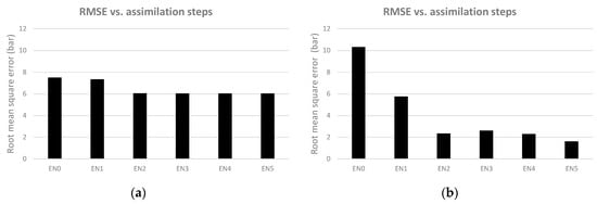
Figure 3.
The root mean square error (RMSE) for the history-matching quality over the assimilation steps, geological scenario mix. (a) Results with Monte Carlos sampling; (b) and the sampling procedure proposed by the author.
Figure 4 shows the observed data coverage by alternatively generated initial ensembles. The Monte Carlo sampling procedure, presented to the left, does not provide optimistic and pessimistic realizations within the initial ensemble. The solution introduced by the author provided coverage of the observed data, giving a favourable environment for efficient algorithm functioning.
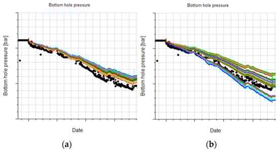
Figure 4.
The coverage of observed data (black dots) by the initial ensembles. (a) Monte Carlo sampling; (b) proposed sampling procedure.
4.2. Uncertainty around History-Matching Parameters—One Year of Production Data—Scenario Mix
The clustering concept was used to generate Figure 5. The analysis of individual classes for the mixed scenario suggests that the reduction of the aquifer’s strength is needed to improve the history match quality, while the drive part coming from the gas expansion needs to be increased. The minimum and maximum ranges of the four classes indicated high variability among the calibration parameters. The above continued to the third iteration, whereas further assimilation steps reduced the posterior uncertainty around the calibration parameters.
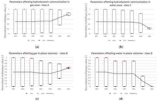
Figure 5.
The change of normalized parameters affecting pressure development in the reservoir, history-matching using one year of production data—geological scenario mix. (a) class A; (b) class C; (c) class B; (d) class D.
4.3. History-Matching—One and Two Years of Production Data—All Aquifer Scenario
Figure 6 indicates that the predictiveness of the models increases with the calibration quality. Moreover, two regression lines can be seen, suggesting that history-matching using two years of production data gives a step increase in predictiveness compared to conditioning with only one year of production history.
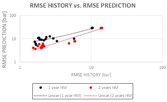
Figure 6.
The relationship between the quality of history-matching and predictiveness of the models.
Figure 7 illustrates that the uncertainty around gas reserves and in-place volumes is a function of the history-matching quality. Together, with improved calibration quality, a reduction of uncertainty for gas reserves and in-place can be seen.
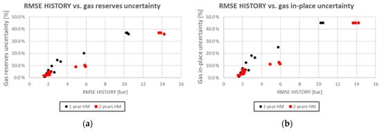
Figure 7.
The impact of history match quality to the modelling uncertainty. (a) Gas reserves, (b) in-place volumes.
Figure 8 and Figure 9 highlight that an unambiguous definition of the aquifer scenarios enabled the determination of a wider range of uncertainty around the gas reserves and in-place volumes. Moreover, the constant presence of an active aquifer generates realizations with the lowest gas in-place volume.
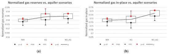
Figure 8.
The uncertainty around the gas reserves and in-place volumes, history-matching using one year of production data and final ensemble with the best history match quality—various aquifer scenarios. (a) Gas reserves, (b) in-place volumes.
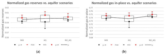
Figure 9.
The uncertainty around the gas reserves and in-place volumes, history-matching using two years of production data and final ensemble with the best history match quality—various aquifer scenarios. (a) Gas reserves, (b) in-place volumes.
Figure 10 and Figure 11 show that for runs with an active aquifer, the history match quality improvement has always been obtained by applying reductions to the strength of the aquifer. For history-matching with two years of production history, the aquifer strength reduction was applied faster in the assimilation process than when only one year of production data was used. Furthermore, the average values of parameters affecting the hydrodynamic communication and in-place volumes for hydrocarbon-saturated regions do not correlate with the aquifer’s strength.
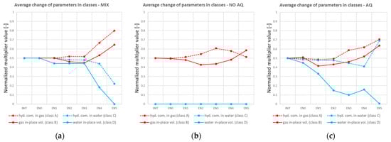
Figure 10.
The average change of parameters during the history-matching, various aquifer scenarios—calibration using one year of production data. (a) Scenario mix; (b) no aquifer; (c) aquifer.
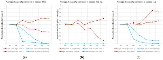
Figure 11.
The average change of parameters during the history-matching, various aquifer scenarios—calibration using two years of production data. (a) Acenario mix; (b) no aquifer; (c) aquifer.
5. Discussion
The optimization of the initial ensemble sampling was performed by application of the two-level full factorial design combined with the clustering concept. This approach provided sufficient variability within the initial ensemble, hence the ES-MDA could search for potential solutions more efficiently and calibrate the models more accurately. Ultimately, the ensemble’s history-matching quality at the fifth assimilation step was improved by 73% compared to the Monte Carlo sampling method. Furthermore, the uncertainty around predictions was reduced from circa 20 down to 2 per cent, leading to a 90% improvement.
Regarding the history match quality improvement for various aquifer scenarios, the average RMSE for models calibrated using one year of production data was reduced from 10.3 down to 1.65 bar, leading to an 84% enhancement. For models calibrated using two years of production history, the average RMSE was reduced from 13.91 down to 1.72 bar. The mentioned change represents an 87.6% improvement. The models with the lowest calibration mismatch lie well within the observed data uncertainty summarized in Table 4. The above proves that the ES-MDA can deliver a decent history match quality.
The updates proposed by the ES-MDA usually lead to a reduction of the aquifer’s strength. Moreover, the models with the active aquifer have smaller gas in-place volumes. This observation is explained by the fact that the aquifer delivers additional energy to the system, giving the possibility to replicate the historical pressures in models with lower gas in-place volumes.
The average variability of the parameters controlling the hydrodynamic communication and in-place volume of gas does not correlate with the aquifer’s strength. The above observation explains the fact that the gas in-place volumes can be distributed across the reservoir in several alternative ways, combined with suitable permeability and faults transmissibility modifications. This effect highlights Figure 5, which was created using the data clustering concept. Figure 5 illustrates that the ranges of history-matching parameters are similar to the initial ensemble through the assimilation steps, while the RMSE decreases as per Figure 2. The fifth iteration does not follow the above trend because the observed data uncertainty was not included in conditioning at this step. Thanks to this change, the algorithm provided strong updates, leading to variability reduction of history-matching parameters.
The validation of calibrated models using the remaining three years of production history has shown that calibration using two years of production data increases the predictiveness of the ensemble. The models calibrated using two years of production history generally have higher reserves, in-place volumes and limited aquifer strength compared to the models calibrated using only the first year of production. In addition, the models calibrated with two years of production at the fifth assimilation step have higher uncertainty around gas reserves and in-place volumes. This situation can be explained by a slightly worse history match quality compared to the models calibrated with one year of production data.
The uncertainty associated with the gas in-place volumes and reserves correlates with the history match quality. This observation explains a reduction of solutions variability with a history match quality increase, as demonstrated in Figure 5. Less variability means fewer alternative forecasts, hence narrower modelling uncertainty. For an average RMSE of 2 bar, the uncertainty span of the gas in-place volume and reserves is at the level of nine per cent, while for the RMSE of 1.6 bar, the same uncertainty is around one per cent. All of the above illustrates the high importance of the observed data uncertainty quantification before conditioning the ensemble of models.
6. Conclusions
The ES-MDA has proven to be a useful tool for history-matching and uncertainty quantification problems concerning the real gas-condensate reservoir.
The method for the initial ensemble sampling proposed by the authors improved the efficiency of the ES-MDA algorithm. Ultimately, a 73% increase in the calibration quality was obtained versus Monte Carlo sampling. Better calibration leads to a 90% reduction of uncertainty around gas in-place volumes and reserves.
The clustering concept enabled the more efficient analysis of the history-matching results. The ability to trace global parameters governing the uncertainty improved the understanding of the modelling results.
The author believes that a similar approach for the initial ensemble sampling and results analysis can apply to more complex history-matching cases. However, the number of proposed classes and assumptions around the two-level full factorial design has to be optimized.
The results for various aquifer scenarios demonstrate that more efficient mapping of modelling uncertainty is possible when the main parameters controlling reservoir behavior are identified. Furthermore, the ES-MDA should be used as a verification tool for multiple geological hypotheses, instead of a black box.
Author Contributions
Conceptualization, T.T.; methodology, T.T.; software, T.T.; validation, T.T.; writing—original draft preparation, T.T. and J.S.; writing—review and editing, T.T. and J.S.; supervision, J.S. All authors have read and agreed to the published version of the manuscript.
Funding
This research received no external funding.
Conflicts of Interest
The authors declare no conflict of interest.
Nomenclature
| EnKF | ensemble Kalman filter |
| ES | ensemble smoother |
| ES-MDA | ensemble smoother with multiple data assimilation |
| probability distribution function | |
| MIX | maximum value |
| MIN | minimum value |
| RMSE | root mean square error |
| RMSE History | root mean square error, used to quantify the history-matching quality |
| RMSE Prediction | root mean square error, calculated using validation data set to quantify the predictiveness of the models |
| INIT | initial range of parameters created based on available geological documentation |
| EN0 | initial ensemble creased by sampling predefined history-matching parameters |
| EN1, EN2…EN5 | the ensemble of models at a certain assimilation step |
| Perm_M(1) to Perm_M(23) | the value of the permeability multiplier in regions from 1 to 23 |
| PV_M(1) to PV(23) | the value of the pore volume multiplier in regions from 1 to 23 |
| Fault(1) to Fault(8) | the value of the transmissibility multiplier associated with the faults from 1 to 8 |
References
- Janiga, D.; Podsobiński, D.; Wojnarowski, P.; Stopa, J. End-point model for optimization of multilateral well placement in hydrocarbon field developments. Energies 2020, 13, 3926. [Google Scholar] [CrossRef]
- Brantson, E.T.; Ju, B.; Omisore, B.O.; Wu, D.; Selase, A.E.; Liu, N. Development of machine learning predictive models for history matching tight gas carbonate reservoir production profiles. J. Geophys. Eng. 2018, 15, 2235–2251. [Google Scholar] [CrossRef]
- Jerzy Stopa, S.R.; Wojnarowski, P. Wykorzystanie wyników symulaji komputerowej do oceny efektywności udostępnienia złoża ropy naftowej za pomocą otworów horyzontalnych. Nafta-Gaz 2008, 679–688. [Google Scholar]
- Heidari, L.; Gervais, V.; Le Ravalec, M.; Wackernagel, H. History matching of reservoir models by ensemble kalman filtering: The state of the art and a sensitivity study. AAPG Mem. 2011, Vol. 96, 249–264. [Google Scholar] [CrossRef]
- Haldorsen, H.H.; Damsleth, E. Stochastic Modeling (includes associated papers 21,255 and 21,299). J. Pet. Technol. 1990, 42, 404–412. [Google Scholar] [CrossRef]
- Bratvold, R.B.; Mohus, E.; Petutschnig, D.; Bickel, E. Production Forecasting: Optimistic and Overconfident—Over and Over Again. SPE Reserv. Eval. Eng. 2020, 23, 0799–0810. [Google Scholar] [CrossRef]
- Yang, C.; Nghiem, L.; Card, C.; Bremeier, M. Reservoir model uncertainty quantification through computer-assisted history matching. In Proceedings of the SPE Annual Technical Conference and Exhibition, Anaheim, CA, USA, 11–14 November 2007; Volume 2, pp. 1121–1132. [Google Scholar]
- Hoffimann, J. The Inverse Problem of History Matching—A Probabilistic Framework For Reservoir Characterization And Real Time Updating. 2014. Available online: https://www.researchgate.net/publication/271507123_The_Inverse_Problem_of_History_Matching_-_A_Probabilistic_Framework_for_Reservoir_Characterization_and_Real_Time_Updating (accessed on 30 May 2022).
- Oliver, D.S.; He, N.; Reynolds, A.S. Conditioning Permeability Fields to Pressure Data; European Association of Geoscientists & Engineers: Brussels, Belgium, 1996. [Google Scholar] [CrossRef]
- Borregales Reverón, M.A.; Holm, H.H.; Møyner, O.; Krogstad, S.; Lie, K.A. Numerical comparison between ES-MDA and gradient-based optimization for history matching of reduced reservoir models. In SPE Reservoir Simulation Conference; OnePetro: Richardson, TX, USA, 2021. [Google Scholar] [CrossRef]
- Emerick, A.A.; Reynolds, A.C. Ensemble smoother with multiple data assimilation. Comput. Geosci. 2013, 55, 3–15. [Google Scholar] [CrossRef]
- Evensen, G.; Hove, J.; Meisingset, H.; Reiso, E.; Seim, K.S.; Espelid, Ø. Using the EnKF for Assisted History Matching of a North Sea Reservoir Model; OnePetro: Richardson, TX, USA, 2007. [Google Scholar] [CrossRef]
- Gibbs, J.W. Elementary Principles of Statistical Mechanics. 1902. Available online: https://www.scirp.org/(S(351jmbntvnsjt1aadkposzje))/reference/referencespapers.aspx?referenceid=1519525 (accessed on 5 August 2022).
- Solheim, D.A. History Matching of the Norne Field Using the Ensemble Based Reservoir Tool (EnKF/ES). 2014. Available online: https://ntnuopen.ntnu.no/ntnu-xmlui/handle/11250/240311?show=full (accessed on 15 May 2022).
- Tveteraas, Ø.; Vey, G.; Hjellbakk, A.; Wojnar, K. Implementation of ensemble-based reservoir modelling on the Ærfugl field. In SPE Norway Subsurface Conference; OnePetro: Richardson, TX, USA, 2020. [Google Scholar] [CrossRef]
- Emerick, A.A.; Reynolds, A.C. Investigation of the sampling performance of ensemble-based methods with a simple reservoir model. Comput. Geosci. 2013, 17, 325–350. [Google Scholar] [CrossRef]
- Montella, C. The Kalman Filter and Related Algorithms: A Literature Review. 2011. Available online: https://www.researchgate.net/publication/236897001_The_Kalman_Filter_and_Related_Algorithms_A_Literature_Review (accessed on 19 July 2022).
- Aanonsen, S.I.; Nævdal, G.; Oliver, D.S.; Reynolds, A.C.; Vallès, B. The Ensemble Kalman Filter in Reservoir Engineering—A Review. SPE J. 2009, 14, 393–412. [Google Scholar] [CrossRef]
- Evensen, G. Sampling strategies and square root analysis schemes for the EnKF. Ocean Dyn. 2004, 54, 539–560. [Google Scholar] [CrossRef]
- Oliver, D.S.; Chen, Y. Improved initial sampling for the ensemble Kalman filter. Comput. Geosci. 2008, 13, 13–27. [Google Scholar] [CrossRef]
- Fevang, Ø.; Singh, K.; Whitson, C.H. Guidelines for choosing compositional and black-oil models for volatile oil and gas-condensate reservoirs. In Proceedings of the SPE Reservoir Engineering (Society of Petroleum Engineers), Dallas, TX, USA, 1–4 October 2000; Society of Petroleum Engineers: Richardson, TX, USA, 2000; pp. 373–388. [Google Scholar]
- Konoshonkin, D.; Shishaev, G.; Matveev, I.; Volkova, A.; Rukavishnikov, V.; Demyanov, V.; Belozerov, B. Machine learning clustering of reservoir heterogeneity with petrophysical and production data. In SPE Europec; OnePetro: Richardson, TX, USA, 2020. [Google Scholar] [CrossRef]
- Tuczyński, T.; Podsobiński, D.; Stopa, J. NAFTA-GAZ Wpływ rezydualnego nasycenia gazem poniżej stwierdzonego kontaktu woda-gaz na proces eksploatacji złoża (Impact of residual gas saturation below the specified water-gas contact on the production process). Nafta-Gaz 2020, 76, 585–591. [Google Scholar] [CrossRef]
- Zavaleta, S.; Adrian, P.M.; Michel, R.M. Estimation of OGIP in a water-drive gas reservoir coupling dynamic material balance and Fetkovich Aquifer Model. In Proceedings of the SPE Trinidad and Tobago Section Energy Resources Conference, Port of Spain, Trinidad and Tobago, 25–26 June 2018. [Google Scholar] [CrossRef]
- Sulaksana, A.; Cheers, M.; Dols, H.; Yap, V. Novel Reservoir Modeling and Experimental Design Approach to Tackle the Challenge of Modeling Highly Compartmentalized Reservoirs under Large Uncertainties in a Mature Offshore Field, Malaysia. In Proceedings of the Abu Dhabi International Petroleum Exhibition & Conference, Abu Dhabi, United Arab Emirates, 13–16 November 2017. [Google Scholar] [CrossRef]
Disclaimer/Publisher’s Note: The statements, opinions and data contained in all publications are solely those of the individual author(s) and contributor(s) and not of MDPI and/or the editor(s). MDPI and/or the editor(s) disclaim responsibility for any injury to people or property resulting from any ideas, methods, instructions or products referred to in the content. |
© 2023 by the authors. Licensee MDPI, Basel, Switzerland. This article is an open access article distributed under the terms and conditions of the Creative Commons Attribution (CC BY) license (https://creativecommons.org/licenses/by/4.0/).