3D CFD Modelling of Performance of a Vertical Axis Turbine

Abstract

Recently, wind turbine research has switched focus to vertical axis wind turbines due to the extensive research that has been performed on horizontal axis wind turbines and the potential of vertical axis wind turbines in built-up areas. This study aims to analyse the performance of a small-scale hybrid vertical axis wind turbine that can switch from functioning as a Darrieus (lift) turbine to a Savonius (drag) turbine by rotating the blades. The turbine was analysed using 3D computational fluid dynamics (CFD) simulations in ANSYS Fluent as the primary method, and the findings were verified using wind tunnel experiments. During the analysis, design parameters such as the blade length, diameter, and number of blades were varied to determine if the design had room for improvement. It was found that the current design of the turbine has an optimal efficiency of 12.5% in the Darrieus configuration, which was found to increase when the diameter or blade length was increased. The Savonius configuration was found to be more efficient at low tip-speed ratios (<0.14), and its efficiency could be increased by adding more blades. The experiments found similar trends to the simulations; however, the efficiencies obtained were on average a tenfold increase from the simulation. Implementing the changes that increased efficiency leads to an increased wake recovery distance, making it less suitable for use in a wind farm.

1. Introduction

Wind has become a favoured source of renewable energy during the transition away from fossil fuels for countries that frequently see windy weather. The most common method of harvesting this energy is using a wind turbine. However, the current procedure of building large wind farms with horizontal axis wind turbines (HAWTs) has its limits. These wind farms can only be built in rural land or off-shore due to their size. Building on-shore is preferred due to its lower costs; however, there is not sufficient land available for countries to be wholly reliant on energy from on-shore wind farms. Due to the high cost of off-shore wind farms, research into how to exploit the wind energy in areas unsuitable for HAWTs has recently gained traction [1].

This research includes a renewed look at vertical axis wind turbines (VAWTs) after research was mostly discontinued in the 1980s in favour of the successful HAWT. VAWTs are more suitable than HAWTs for the built environment due to their low sound emissions from low operational speeds, their omnidirectional wind harvesting without changing the configuration, and their aesthetics that can be incorporated into architecture [2,3]. In the VAWT sector, there are two prevalent designs: a lift (Darrieus) turbine, which operates at high speeds with low torque, and a drag (Savonius) turbine, which operates at low speeds with high torque. Darrieus turbines require the use of an external starting mechanism, while Savonius turbines are self-starting. These characteristics lend towards Savonius turbines being more suitable for turbulent and stormy conditions [3]. Recently, research has been conducted into hybrid designs that combine the benefits of the Savonius and Darrieus turbines [4,5].

Traditionally new turbine designs would be tested using scale models in wind tunnels. However, the process of building models and making alterations to test different parameters can be costly and time-consuming. This has led to computer simulations being integrated as a new step of the design process. Simulations allow for the design to be optimised before performing experiments.

The focus of this research is to provide a performance analysis of a VAWT [6,7] that is capable of operation in a Darrieus and Savonius configuration. Previous research on this design has focused on the use of 2D simulations and wind tunnel experiments; therefore, this research seeks to provide further analysis using 3D simulations.

2. Background

2.1. Vertical Axis Wind Turbine

Wind turbines are machines that convert the kinetic energy available in wind into a torque that is used to generate electricity. VAWTs are wind turbines that rotate about a vertical axis, where the vertical axis to normal to the ground in most cases. In comparison, HAWTs rotate about a horizontal axis, which is parallel to the ground and wind direction. As opposed to the HAWT, the VAWT is not restricted by the direction of the wind making them omnidirectional.

2.2. Darrieus Turbine

The Darrieus (lift) turbine makes use of lift forces to create torque. The lift force is obtained when wind flows over aerofoils attached to the centre with struts, also creating drag forces. The forces are caused by a difference in pressure and wind speed over the top and bottom sides of the aerofoil, which appears when the path length of each side differs. The lift force is generated on the side with the longer path from the leading edge to the trailing edge. The difference in path length can come about from an asymmetric design of the aerofoil or the angle of attack changing.

The Darrieus turbine utilised the lift force to rotate the blades about the vertical axis. The blade will rotate when the results of the lift and drag force have components acting in the direction of motion and towards the centre of rotation. However, after the blade has rotated to a point where the angle of attack results in a weak lift force, the blade will no longer rotate. To overcome this, most designs use multiple blades to ensure there is always a blade producing a sufficient lift force for rotation.

The lift force on the blade is weak at low wind speeds, which can be strong enough to continue the turbine rotation. However, a stronger lift force is required to overcome the initial inertia. Therefore, Darrieus turbines use an external means of starting the rotations, increasing the rotational speed to a point where the lift from the blades can take over. The ability to self-start is further reduced by Darrieus turbines commonly using symmetrical aerofoils, requiring the angle of attack to be changing to produce significant lift. However, symmetrical aerofoils are used, as they display an increased performance during ideal operation [8]. The Darrieus turbine is classified as omnidirectional, as the rotation of the blades will cover the optimal angle of attack for all wind directions during the rotation.

2.3. Savonius Turbine

The Savonius (drag) turbine uses the drag force from the wind to create the driving torque. This is achieved by using cup-shaped blades that are designed to provide a large surface for the wind to push against. The cup shape also partially traps the air until the blade has rotated. Since Savonius turbines utilize the drag force, which is stronger than the lift force at low speeds, they can start with only the force from the wind. Additionally, the use of drag makes it more suitable for a lower range of wind speeds than the Darrieus turbine.

There are many variations to the design of the Savonius turbine, one of which is the Bach turbine. This design uses 2 large cup-shaped blades instead of multiple small blades. A single S-shaped pair of blades only covers wind coming from two directions; therefore, to make the turbine omnidirectional, multiple pairs of blades are stacked with an angle offset. These blades can overlap at the centre of the turbine, allowing some wind to backflow into the returning blade, producing a small increase in positive torque, and improving performance [3].

2.4. Hybrid Turbines

Hybrid turbines try to combine the benefits of the Savonius and Darrieus turbines to obtain a larger operational range of wind speeds and to improve efficiency. Antar, El Cheikh, and Elkhoury [4] proposed a design that is focused on increasing the operational range and efficiency while maintaining a low cut-in wind velocity, the speed at which the turbine can start producing electricity. The design consists of four aerofoils that make up a Darrieus turbine, which can be moved and rotated to create a Savonius turbine with two blades. This allows the turbine to use the better performance of a Savonius turbine at low speeds, then transition into a Darrieus turbine for higher speeds. It was found to successfully improve the efficiency and operational range in simulations. However, the design has a drawback of an increased number of failure points from the increased complexity.

A more common hybrid design explored by Hosseini and Goudarzi [5] consists of a simpler design where a Bach turbine is attached to the centre of a Darrieus turbine. The aim of this design was to achieve an increased operational range and self-starting capabilities compared to the Darrieus turbine by itself. Through simulations, it was found that the turbine successfully increased the operational range and initial torque; however, its efficiency is below that of the unmodified Darrieus turbine.

More recent designs that have been explored include a blade that can open into a V shape, transitioning from Darrieus to Savonius (by Gao, Lian, and Yan [9]) and a double-Darrieus design that has a smaller Darrieus turbine within a larger Darrieus turbine (by Ahmed et al. [10]).

2.5. Turbulence

VAWTs are usually designed for wind that is mostly laminar. However, this is not always the case, as some VAWTs could be deployed in areas with turbulent conditions, resulting in frequent changes to wind speed and direction. Within rural areas, these conditions are observed in mountainous regions, while it is prevalent in urban areas due to the interference of buildings and other structures. It has been found that at low wind speeds, turbulence can be beneficial to the performance of a VAWT, however high turbulence intensity or turbulence at high wind speeds is detrimental [11].

The blades and structure of the VAWT also induce turbulence, where the viscous interaction between the wind and blades leads to the formation of vortices. Large vortices that form at low tip-speed ratios (TSRs) create dynamic stall, where the vortices on the lift surface interfere with the lift force, resulting in a small increase in lift followed by a dramatic decrease [12].

2.6. Analysis Parameters

The aerofoil can be analysed using the lift and drag forces, which can be compared using the lift-to-drag ratio. It is desirable for an aerofoil to have a higher ratio, as it will provide greater efficiency for the turbine.

$$Lift to Drag Ratio = \frac{L}{D}=\frac{F_L}{F_D}$$

(1)

where: $L$ and $F_L$ are the lift force, and $D$ and $F_D$ are the drag force.

The VAWT is mainly analysed using its power and efficiency. The output power is a function of the turning moments (torque) acting on the turbine and the rotational speed, and the input power is the power available in the wind. The efficiency is described using the coefficient of performance (power), which is the ratio of output power to input power, stating the fraction of the available power that can be harnessed by the VAWT.

$$P_t=M\omega$$

(2)

$$P_w=\frac{1}{2}\rho A{v}^3$$

(3)

$$C_p=\frac{P_t}{P_w}=\frac{2M\omega }{\rho A{v}^3}$$

(4)

where $P_t$ is the turbine power; $M$ is the moment or turning force; $\omega$ is the rotational speed; $P_w$ is wind power; $\rho$ is the density of air; $A$ is the projected (frontal) area of the turbine; $v$ is the wind velocity; and $C_p$ is the coefficient of performance.

Equation (4) has two main variable parameters, the wind speed, and the rotational speed. Varying these parameters allow for a power curve to be constructed for a turbine. These parameters can also be combined into a single parameter, the tip-speed ratio, the ratio between the speed at the blade tips, and the wind speed. This parameter can be inserted into the coefficient of performance equation using the moment coefficient.

$$TSR=\lambda =\frac{\omega R}{v}$$

(5)

$$C_m=\frac{M}{\frac{1}{2}\rho v^{2}Al}$$

(6)

$$C_p=\frac{\omega l}{v}{C}_m=\lambda C_m$$

(7)

where $TSR$ and $\lambda$ is the tip-speed ratio of the turbine; $R$ is the turbine radius; $C_m$ is the moment coefficient; and $l$ is the distance from centre of rotation to the moment, e.g., the radius.

Turbines are also described using their solidity, which relates the number and size of blades, to the turbine diameter.

$$\sigma =\frac{nc}{D}$$

(8)

where: $\sigma$ is solidity; $n$ is the number of blades; $c$ is the chord length; and $D$ is the turbine diameter.

2.7. Simulations

Simulations of wind turbines consist of using computers to solve numerical methods of predicting the air flow around the turbine. Computers are used due to the large number of repetitive calculations required to get an accurate prediction. This numerical analysis is referred to as computational fluid dynamics (CFD). CFD software solves a set of equations that describe the air flow, determined by the turbulence model, using the finite volume method. There are two commonly used CFD software for VAWTs, ANSYS Fluent [1,4,5,6,7,12,13,14,15,16,17,18,19,20,21,22,23,24] and STAR-CCM+ [1,2,23,25].

2.7.1. 2D and 3D

Simulations are commonly performed using a 2D model of the cross-section of a turbine’s blades. This is due to the fact that a simpler model results in fast simulation times while maintaining reasonable accuracy [4,8]. However, when high accuracy and a realistic representation is desired, a 3D model is more suitable. 3D models tend to be used when the full turbine is modelled in later stages of design. The decreased accuracy from 2D simulations is related to inaccurate prediction of the following 3D phenomena: dynamic stall and vortex shedding [13,22,26]; wake produced by the central tower [20,21,22,26]; parasitic drag from features excluded features [8,19,22]; curvature of the flow [19]; and finite blade effects [8,19,20,22].

2.7.2. Turbulence Models

The commonly used turbulence models are based on the Unsteady Reynolds-Averaged Navier Stokes (URANS) due to their fast simulation times [24], of which the three most used are k-ω Shear Stress Transport (SST k-ω) [1,5,6,11,14,16,17,18,22,23,25,27], k-ε Realizable [3,8,24], and Transition SST [8,20,23,25]. SST k-ω and k-ε Realizable are second-order models, and Transition SST is a more complex third-order model. Barnes [23] found from comparing five URANS models for 2D CFD simulations that the Transition SST model provided the most accurate results compared to experimental data. However, it also has the longest simulation, leading to the model with the next best accuracy and a fast simulation time, SST k-ω, being recommended.

There are also other commonly used models, such as the third-order models, Large Eddy Simulation (LES) [27], and Detached Eddy Simulation (DES) [12,20]. These models have been found to be more accurate than URANS-based models, especially during dynamic stall [27], at the cost of longer simulation times. There are also simpler simulation methods such as the first order model, Spalart-Allmaras (S-A) [12,19], or laminar flow [18].

2.7.3. Convergence

When running a simulation, it is best practice to optimise the model to obtain a balance between accuracy and simulation time. The main focuses of optimisation are the mesh of the flow domain and the timestep. Mesh convergence is determined by performing simulations with different densities and comparing the values obtained for chosen parameters and the simulation time, to determine a reasonable simulation time for the desired accuracy. Timestep convergence consists of altering the timestep instead of mesh density. A reasonable timestep can also be determined with the Courant-Friedrichs-Lewy criterion [24]. It uses the element sizes at the interface between stationary and rotating zones to determine the timestep based on the chosen Courant number. The Courant number should be at the highest one and more commonly 0.5, with Trivellato [24] suggesting 0.15.

$$C_{FL}=\frac{u\mathrm{\Delta }t}{\mathrm{\Delta }x}<1$$

(9)

where $C_{FL}$ is the Courant number; $u$ is the local flow velocity at the grid element; $\mathrm{\Delta }t$ is the temporal discretisation (timestep); and $\mathrm{\Delta }x$ is the spatial discretisation (element size).

2.7.4. Simulation Analysis

When the performance of the turbine is of interest, then a power curve will be used to demonstrate performance at a range of conditions, with the performance averaged over a full rotation. The performance can also be analysed by observing the turbine’s wake, using contours showing the velocity, pressure, or turbulence.

2.8. Experiments

VAWT experiments consist of testing scaled modes in wind tunnels. Wind tunnels simulate wind by using fans that can be controlled to vary the wind speed. They also use a converging design to promote laminar flow conditions in the test area. The performance data can be calculated using the torque obtained from a torque meter attached to the VAWT shaft and the shaft’s rotational speed. The wake can be understood through multiple methods, with the simplest being measuring the velocity upstream and downstream of the turbine using anemometers, laser and acoustic Doppler velocimetry, or Cobra probes [24]. The wake can be visualised using more complex methods such as Particle image velocimetry or using a smoke machine, which is recorded with a camera [2,23,28].

2.9. Previous Work on the VAWT Design

Durkacz et al. [6] used a larger-scale version of the turbine used in this work. They investigated the turbine’s use as a central turbine in a planetary formation, with three smaller outer turbines. It was found that at the optimum TSR, the efficiency increased by 1%, with an average increase of 4% across the full TSR range. The simulation results were verified by scaled wind tunnel tests identifying the same trends.

3. Simulation Methodology

ANSYS Workbench 2021 R1 was used for the full simulation process, with DesignModeler used for geometry, ANSYS Meshing for the mesh, and Fluent for solving. This software was chosen based on the authors’ familiarity and its widespread use. The simulations followed these overarching steps:

• Creating simplified geometry and domain.
• Meshing the domain.
• Setting up the solver and performing the simulation.
• Extracting data.

3.1. Single Blade/Aerofoil

The geometry comprises solids that fill the fluid domain, with the aerofoil cut out, shown in Figure 1. This was done as only the walls describing the outer shape of the aerofoil will interact with the flow. The aerofoil is NACA 7715 with 250 mm chord length and 250 mm span. The domain was set to give a spacing of 5c (5 × chord length) around the aerofoil, to allow the flow to develop. The outer bounds of the domain are a cylinder with a diameter of 11c (2.75 m) and height of 11c (2.75 m). The domain has been further split up to allow for more control in meshing.

The mesh uses the multizone meshing method, with hexahedron-mapped meshes and tetrahedron-free meshes to allow zones to be assigned different mapping styles. Additionally, body sizing and inflation have been used to make the mesh denser around the aerofoil. Three mesh sizes were created: 1 million elements, 0.5 million elements, and 1.4 million elements.

The solver was set to use the SST k-ω turbulence model, chosen due to its frequent use in literature, good accuracy, and relatively short simulation time, as observed in Section 2.7.2. The material of the fluid domain was set as air. The inlet’s boundary condition is velocity inlet with turbulent intensity of 5% and turbulent length scale of 1 m. The outlet is a pressure outlet with the same turbulent parameters as the inlet. The inlet and outlet conditions are based on the setup by Durkacz [6]. The walls have been set as symmetry boundaries, and the aerofoil faces are no-slip walls. The reference values were set as shown in

Table 1. Reference values for single blade simulation.

Parameter	Value
Area 1	0.0625 m2
Density	1.225 kg/m3
Enthalpy	0 J/kg
Length	0.25 m
Pressure	0 Pa
Temperature	288.16 K
Velocity 2	10 m/s
Viscosity	1.7894 × 10−5 kg/(m s)
Ratio of specific heats	1.4
Yplus for Heat Tran. Coef.	300

¹ The reference area is the projected area of the aerofoil. ² The reference velocity was changed to match the wind velocity of the current simulation.

. The simulation was set as steady-state and set to end after 500 iterations or when all the residuals reach 1 × 10⁻⁵.

The solver was set up to output the drag force, lift force, drag coefficient, and lift coefficient in the console at the end of the simulation. All three meshes were simulated to determine an optimal mesh, which was then used to simulate wind speeds of 10 m/s and 8 m/s with angle of attack ranging from +5° to −5° (obtained by rotating aerofoil geometry). The method of determining the suitability of the mesh consisted of comparing output parameters such as drag and lift, for three different mesh densities ranging from 500k elements to 1.4 million elements. This was then compared to the duration of the simulation to obtain good accuracy within a reasonable timeframe. The changes in mesh densities consisted of changing all element sizes by the same factor, e.g., multiplying all sizes by 0.75 to obtain a denser mesh.

3.2. VAWT

The geometry was created with the parameters in

Table 2. VAWT geometry.

Parameter	Value
VAWT type	Darrieus
No. of blades	3
Chord length	100 mm
Blade height	260 mm
Rotor diameter	200 mm
Domain length (X)	4 m
Domain width (Y)	2.2 m
Domain height (Z)	2.26 m

.

The domain size is equivalent to 20D × 11D × (10D + L), shown in Figure 2. This provides sufficient area for flow to develop before and after the turbine and reduces interference from outer boundaries. Similar domains have been used in literature, producing satisfactory results [13,20]. The geometry has been split into a stationary zone and rotating zone using a cylinder. The mesh has been further split up to assist in refining the mesh.

The geometry of the Darrieus turbine was altered to create designs with blade heights of 200 mm and 320 mm, and diameters of 150 mm and 250 mm. The blades were also rotated 90° to create a Savonius configuration, and additional blades were added (Figure 3).

Based on the mesh convergence for the single blade (Section 5.1), it was determined that a mesh of one million or more elements is suitable. The mesh used the same techniques as the single blade, with additional techniques of face sizing and automatic method used for complex geometry near the blades. The mesh contains roughly 1.4 million elements (Figure 4), going up to 2.3 million elements for the five-blade Savonius turbine. The orthogonal quality of the meshes was kept below 0.01 to avoid floating point errors in the simulations.

All the configurations used the same setup values (

Table 3. VAWT solver values.

Parameter	Value
Time	Transient
Turbulence model	SST k-$\omega$
Area	0.052 m2
Density	1.225 kg/m3
Enthalpy	0 J/kg
Length	0.1 m
Pressure	0 Pa
Temperature	288.16 K
Velocity	12 m/s
Viscosity	1.7894 × 10−5 kg/(m s)
Ratio of specific heats	1.4
Yplus for Heat Tran. Coef.	300
Inlet turbulent intensity	2%
Inlet turbulent length scale	0.02 m
Outlet turbulent intensity	2.2%
Outlet turbulent viscosity ratio	0.1
No. of timesteps	900
Iterations per timestep	20

), with some values changed to match the parameters of the current simulation. The simulations were performed with a transient time model to allow for analysis at different points of the rotation and to obtain an average throughout a rotation.

The boundary conditions are mostly the same as in the single blade simulation, with the key differences being that the inner domain was set to rotate about the Z axis with a rotational velocity, ω, and the walls within the inner domain and the interfaces were given the same rotational speed. The inlet and outlet settings were based on a similar simulation [6]. The timestep was set to be equal to a rotation of 2°. This was obtained through Equation (9) for a case with 12 m/s wind and rotating at 120 rad/s. The step is too high to make the 0.15 Courant number criterion, but it stays below the more common criterion of 0.5.

The data was obtained in the form of contours on the XY plane through the centre of the turbine, every two timesteps which were saved as jpegs, and data values were obtained every timestep and exported as text files. The data values of concern were the moments and moment coefficients. The contours were velocity, pressure, turbulent kinetic energy (TKE), vorticity magnitude, and Z-vorticity. The simulations of the Darrieus turbine were performed for multiple tip-speed ratios for varied wind speeds. The altered Darrieus turbines were only simulated at 14 m/s wind speed, and the Savonius configurations were simulated at 6 m/s wind speed, with the three-blade configuration also being simulated at 12 m/s to allow comparison between Darrieus and Savonius.

4. Experiment Methodology

The purpose of the experiments is to provide a point of comparison for the simulations and to determine how realistic the simulations were.

4.1. Single Blade/Aerofoil

A pre-existing model with the same dimensions as the model from the simulations was used. The model was connected to a three-point balance (Figure 5) using a cylindrical rod on the inside of the wind tunnel, allowing the lift and drag to be obtained with software. The model was located within the wind tunnel. The experiment consisted of running at a wind speed of 6 m/s and 12 m/s and changing the angle of attack of the aerofoil. The lift and drag were obtained ten times over a period of 20 s, so an average could be calculated.

4.2. VAWT

The model used for the VAWT experiments is of the same scale as the simulations. The model was constructed by previous researchers with a wooden frame and 3D-printed blades. The model was located at the end of the wind tunnel, as shown in Figure 6. The model has breaks attached to the top of the central shaft that could be applied by tightening nuts. The shaft was connected to a torque meter below the frame. Tape was attached to the blades to prevent them from rotating.

The experiment consisted of running the wind tunnel at its maximum speed (roughly 14 m/s) and a slightly slower speed (roughly 12 m/s), for three brake tightness variations. The brakes were used to alter the rotational speed of the turbine. Lower wind speeds were not tested for the Darrieus configuration as the model could not continue rotation unassisted. The Savonius configuration was tested at wind speeds of 8, 10, and 12 m/s. The average wind speeds at the exit as well as at further distances downstream were measured using an anemometer. The torque was obtained using the torque meter, connected to a computer through a controller. A smoke machine was used to show the flow, which was recorded with a camera.

5. Simulation Results and Discussion

5.1. Single Blade/Aerofoil

Table 4. Mesh validation.

Elements	Duration	Drag Coefficient	Lift Coefficient	Drag (N)	Lift (N)	Iterations
510,124	2 h	0.070788	0.23833	0.27098	0.91236	500
1,013,542	1 h	0.056044	0.21801	0.21454	0.83456	90
1,363,588	1 h	0.055799	0.21802	0.21361	0.83460	88

shows the data obtained from simulating three mesh densities. The values obtained from the roughest mesh differ greatly from the other meshes, along with having the longest duration. This is because the mesh was too coarse for the residual limits to be met before reaching the 500-iteration limit. The other meshes obtained very similar results for similar times; therefore, the mesh is sufficiently converged at one million elements.

Figure 7 shows the results of the single blade simulations using the lift-to-drag ratio. It was found for both wind speeds that reducing the angle of attack would reduce the lift while increasing the drag, with the lift being smaller than drag at −5°, signalled by the ratio dropping below one. Both cases show a similar trend, with a possible optimal ratio at around 3° to 4°; however, more simulations above 5° would be necessary to prove this. The lines do not cross with a trend displayed of a higher ratio for a higher wind speed, with the difference narrowing at higher angles of attack.

5.2. Darrieus Turbine

Two methods of obtaining the coefficient of performance were compared in

Table 5. Coefficient of performance calculation method comparison.

Parameter	Value
WS (m/s)	12	12	12	12	12	12	12
TSR	0.1	0.3	0.5	0.7	0.9	1	1.2
Cp (TSR method)	0.00837	0.048732	0.091961	0.121013	0.109003	0.085687	0.026125
Cp (power method)	0.00837	0.048732	0.091961	0.121013	0.109003	0.085687	0.026125
% Difference	−3.6 × 10−6	−3.6 × 10−6	−3.6 × 10−6	−3.6 × 10−6	−3.6 × 10−6	−3.6 × 10−6	−3.6 × 10−6

. The methods compared were using Equation (7) (TSR method) and performing the full power calculations to justify using the shorter method. The values were compared for simulations at a wind speed of 12 m/s, finding that the values from each were practically the same, with any differences being small enough to designate as rounding errors.

The power coefficients obtained from simulations of the unaltered Darrieus VAWT were plotted in Figure 8. The power curves were found to be the same when compared to the TSR; however, the power curves, when compared to the rotational speed of the turbine, were shifted to the right as the wind speed increased. This means that to maintain optimal performance at a higher wind speed, the rotational speed must be increased. The optimal power coefficient of this design is 0.124 at a TSR of 0.75.

The contours are located along the midplane of the turbine, as shown in Figure 9. The following contours are displayed from above for clarity.

Figure 10 shows the velocity contours obtained at the end of the fifth rotation for the simulations at a wind speed of 14 m/s. As the TSR increases, the wake becomes more symmetrical, due to the turbine starting to act as a cylinder. The lowest TSR shows a wavy wake, which is a sign of how much the wake changes throughout the rotation, while the others have a relatively consistent wake during the full rotation, shown in Figure 11. The spot of highest velocity was found at the leading edge of the blade at an azimuth angle of 120° (anticlockwise from the Y-axis). The velocity was found to have reduced from 0.2 m in front of the turbine to a recovery point downstream, 1.6 m for the highest TSR and greater than 1.84 m for the lowest TSR. Simulations at different wind speeds found that the shape of the wake does not vary with wind speed when the TSR is kept constant, with the only change being the velocities scaling to match the change in wind velocity. Therefore, the wind speed can be estimated using the TSR without specific knowledge of wind speeds and rotational speeds.

The obtained pressure contours for the wind speed of 14 m/s and TSR of 0.7 at different stages of rotation are also shown in Figure 11. It was found that there was no observable change to the pressure in the far wake, hence, the far wake has been excluded from the figures. Instead, all the observable changes for the pressure scale used are localised to the near blade area. The highest and lowest pressures were found on the blade at 90° (leftmost blade at 320° rotation, Figure 11d) of 300 Pa and −600 Pa, respectively. Figure 10 also shows that the pressure increased with the TSR and that larger vortices developed at lower TSRs, with lower pressures. The locations of high pressure coincide with the low-velocity areas at the blade walls, with low pressure coinciding with high velocity.

Figure 10 also shows the TKE at different TSRs for a wind speed of 14 m/s. The TKE wake differs greatly in each scenario. The wake at a TSR of 0.3 (Figure 11c) is very chaotic due to the slower rotation allowing for more air to flow within the turbine area. In this scenario, the flow within the turbines is at a high TKE, like the vortices rolling off the blades in Figure 11. At a TSR of 0.7 and higher, the wake starts to become a wave, and the intensity starts increasing. While the far wake intensity increases, the wake inside the turbine decreases as it begins to act akin to a solid cylinder. Figure 11 shows the TKE at different stages of the rotation. The wake is shown to stay relatively similar, with small fluctuations of energy, shown by some sections slightly changing colour. The greatest energy in the far wake was found in line with the blade-producing lift. The near wake shows vortices rolling off the blade at roughly 10 J/kg. While the vortices are still attached to the blade, the centre can reach 20 kJ/kg.

5.3. Darrieus Turbine Design Optimisation

The results of varying the diameter, and therefore the solidity, are shown in Figure 12a. They were all simulated at the same rotational speeds. This showed that as the diameter increased from 0.15 m to 0.25 m, the curve became larger and shifted to the right. In general, the larger diameter provided better performance, with the only exception being between a TSR of 0.3 and 0.4, where the 0.15 m diameter outperformed the original 0.2 m diameter. These results show that decreasing the solidity of the current design would increase the performance. However, improvement is not guaranteed when operating at a low TSR. These findings are in line with the findings from Mohammed [29], where an increasing solidity narrows the operational range and decreases efficiency. The results of varying the length of the blades are shown in Figure 12b. It shows that all the designs follow a similar curve, which as the length is increased is shifted up. However, the upward shift or increase in performance is not linearly related to the length, as the gap between the curves is not equal, as the increase from 0.20 m to 0.26 m is a 30% increase in diameter for an increase in peak power coefficient of 0.008, while the increase from 0.26 m to 0.32 m is a 23% increase in diameter for an increase of 0.034. Therefore, it is beneficial to increase the blade length; however, in some cases, it may not be economical.

Figure 13 shows the velocity, pressure, and TKE contours obtained for the different diameters. The pressure contour has been cropped to only show the near turbine area, as the scale is too large to observe changes within the far wake. For the velocity the main difference in the wake is that there are lower velocities in the far wake for larger diameters, representing a slower wake recovery. The shape of the wake also changes, with the smaller diameter producing an angled thin wake, while the larger diameter produces a straighter wide wake. The pressure contours show the same wake shape in all cases, with the only difference being an increase in pressure when the diameter increases. The TKE contours show the same change in the shape of the far wake as the velocity contours. They also show that the turbulence increases as the diameter increases. The reason for the differences in wake observed in the velocity and TKE contours is the solidity changing, making it act like a solid cylinder.

Figure 14 shows the contours associated with changing the length of the blades. In this case, the wake shapes for each contour do not change as the length changes; however, the values do change. The velocity range increases as the length increases, with the wake having lower velocities and the vortices having a higher peak velocity. The lower velocity when length increases is due to the central pane being further from the flow above and below the turbine. For the pressure contour, there is not a notable difference in the positive pressures; however, the negative pressure in the vortices has increased. The TKE contours show a trend of increasing TKE with increasing blade length for all non-zero areas.

5.4. Savonius Turbine

A comparison of the power curves for the three-blade Darrieus and Savonius designs at a wind speed of 12 m/s is shown in Figure 15. The Savonius power curve is small in comparison to the Darrieus power curve. However, the Savonius design achieved a higher coefficient of performance for the TSR range of 0.05 to 0.14 and will likely have similar or better performance below 0.05. This shows that the Savonius design is inefficient; however, it is a better choice than the Darrieus turbine for operation at low TSRs.

Figure 16 shows the velocity, pressure, and TKE contours obtained at a wind speed of 6 m/s for different TSRs of the three-blade Savonius design. In the velocity contour, the wake pattern is very different than observed for the Darrieus turbine. One difference is that the main gathering of the velocity deficit has swapped to the negative side of the Y-axis. The wake also becomes more chaotic as the TSR increases, however, as the TSR is much lower, the wake may become less chaotic at higher TSRs. There is a slight increase in velocity observed at the rear of the turbine above the top blade, which could be related to vortices. In all cases, the wake does not substantially recover within the simulation bounds.

All the pressure contours in Figure 16 show a vortex on the rear blade; however, they are at different stages of development, with the TSR of 0.02 having the earliest stage of development, and the TSR of 0.05 having the most developed vortex. The pressure values were highest for the TSR of 0.05 and the lowest for the TSR of 0.1. This does not follow the regular trend found for the Darrieus turbine, where TKE increased with TSR.

The TKE contours in Figure 16 follow a similar trend to the pressure, where the TSR of 0.1 has the lowest turbulence and the TSR of 0.2 has the highest. As opposed to the Darrieus turbine, the TKE wake quickly loses intensity, almost fully dissipating after 0.6 m for all cases. The wake of the TKE follows the same shape as the velocity deficit. The near turbine wake differs for each TSR, maintaining the same shape with different intensity distributions. The TSR of 0.2 has the most turbulence at the blade at 120° (anti-clockwise), while the TSR of 0.05 has greater turbulence at 0°. Meanwhile, the TSR of 0.1 has a similar turbulence at each blade.

5.5. Savonius Turbine Design Optimisation

The comparison between the number of blades on the Savonius turbine is shown in Figure 17. It shows that for a goring from a wind speed of 12 m/s to 6 m/s the performance of the three-blade design slightly decreases. It also shows that increasing the number of blades increases the performance and increases the TSR required for optimal performance. The four-blade design does not follow the standard power curve, having a lower-than-expected power coefficient at the TSR of 0.15. The simulations for the four-blade design were repeated, obtaining the same results, to ensure the unexpected curve was not due to a mistaken input. This curve is not found for other Savonius turbine designs with four blades; hence, the cause is likely related to the aerofoil shape of the blade not being suitable for a four-blade design. The results suggest that the current design would have improved efficiency in the Savonius configuration by increasing the solidity (number of blades).

Figure 18 shows the contours obtained for the Savonius designs, at a TSR of 0.1 and wind speed of 6 m/s. The shape of the wake in the velocity and TKE contours is reminiscent of ocean waves, with the higher number of blades decreasing the wavelength but increasing the frequency (decreasing spacing between the waves). The velocity deficit stays at the minimum for a larger area and takes longer to recover in the five-blade design, due to the increased solidity from increasing the number of blades. In all cases, there is no large increase in velocity. The TKE increased as the blades increased, with the largest increase found near the blades. There is no significant change in the positive pressure in each case; however, the negative pressure and number of vertices does increase.

6. Experimental Results and Discussion

6.1. Single Blade/Aerofoil

Figure 19 shows that the simulations have overestimated the values obtained from the experiment and that the experiments found a shallower curve. Additional simulations were performed at the same speeds as the experiments, displaying similar values and trends to the previous simulations. The experiments suggest that the optimal angle of attack would be above 5° instead of 4°, suggesting that more simulations are required above 5° to find the optimal angle. This is in line with the findings from Wright, Droubi, and Islam [30], where the optimal angle of attack is around 30°. However, the experiment shows the same basic trend of increasing the lift-to-drag ratio as the angle and wind speed are increased. On average the data from simulations predicted a twofold increase for 12 m/s and a fourfold increase for 6 m/s. This difference can be attributed to the surface roughness of the printed model, and the increased drag from the cylindrical rod that the aerofoil is mounted on. The difference could also suggest that the inlet and outlet conditions in the simulation are not representative of the wind tunnel, as increasing the turbulence would increase the lift and drag.

6.2. Darrieus

The data obtained from the experiments are compared with a simulation in Figure 20. At low TSRs, the simulation shows a trend of increasing power coefficient with TSR that is not shown in the experiment, with the average staying around 0.048. The experiment obtained a power coefficient five times higher than the simulation at the highest TSR and almost fifteen times higher at the lowest TSR. To declutter experimental data, the TSRs with less than 5 data points were excluded, the average at each TSR was obtained, then similar TSRs were averaged. The different trends could be related to the frame of the experiment model, and the walls of the wind tunnel. Additionally, for the experiment, the inlet has a smaller area, and the air around the turbine is stagnant, while the simulation has a flow of 12 m/s fully surrounding the turbine. The discrepancies could also be a problem of the simulation struggling to model low TSRs. Additionally, the turbulent conditions set for the inlet and outlet of the simulation may differ from the experiment. A similar underprediction by the simulations was observed by Durkacz et al. [6] when using a similarly designed turbine.

The wind speed data obtained from the experiments at roughly 14 m/s are shown in

Table 6. Wind velocity contours from experiment at two inlet velocities.

Inlet Velocity (m/s)	Y (m)	Wind Speed (m/s)
14.12	0.24		14	12
	0	14.12	Turbine	7.9	6.7	7.2	7.5	8.4
	−0.24		14	12.2
13.86	0.24		13	10.1
	0	13.86	Turbine	9	8.8	8.5	8.2	8.8
	−0.24		15.2	11.9
	X (m)	−0.24	0	0.24	0.365	0.49	0.615	0.740

. This data was chosen for comparison as it was around a TSR of 0.1, allowing it to be compared with the contour in Figure 21. In the simulation of the sides of the turbine at 0.24 m, it is shown that the velocity is equal to or slightly higher than the inlet velocity. Meanwhile, the experiments found similar velocities directly to the side, which decreased downstream. The second set of experimental data showed an increase on one side, which could suggest the presence of turbulent flow. However, these discrepancies and the turbulent flow may not be a direct result of the turbine, instead being caused by the frame the model was mounted to and the lower surrounding wind speed. The simulation and experiments agree, with the downstream wake at the measured points having similar velocities that are gradually recovering.

Two of the clearest images from using the smoke machine are shown in Figure 22. The nozzle of the smoke machine is shown in Figure 22a, to the left of the spinning turbine, with a black surface placed below the turbine to improve visibility. The smoke shows that the air is flowing around the turbine on the returning side. As the smoke approaches the turbine it is diverted before colliding with the blades, showing that there is little flow at the front of the turbine, which agrees with the low velocity and high pressure shown by simulations. The flow is also shown to split on the trailing edge of a returning blade, creating a swirling pattern on the outer side of the blade. This shows the presence of a vortex which agrees with the velocity and TKE contours from the simulations. Most of these findings are also demonstrated in the streamlines shown in Figure 23. However, there is one main difference: the streamlines do not show the flow around the side entering the turbine; instead, flow with the turbine all comes from the front. This may also be the case for the experiment; however, the image does not have the clarity to determine this.

6.3. Savonius

The experimental and simulation data for the three-blade design are shown in Figure 24. The simulations at two different speeds showed that increasing the wind speed provides a slight increase in performance while maintaining a similar curve. The experiment data produced a power curve with a peak power coefficient of 0.13 at a TSR of 0.15. This peak value is almost tenfold what was found in the simulations. Additionally, the experiment found a shallower curve, suggesting a greater operational TSR range than found in the simulations. This is also shown by a large power coefficient obtained from the experiment at a TSR of 0.24, while the simulations are no longer operational (Cp < 0).

7. Conclusions and Recommendations for Further Research

With the aim of understanding the performance and wake characteristics of the VAWT design, 3D simulations and experiments were performed. These consisted of altering operational and design parameters, including changing from a Darrieus to Savonius configuration, to further our understanding of whether the current design can be improved. The conclusions obtained from this research are as follows.

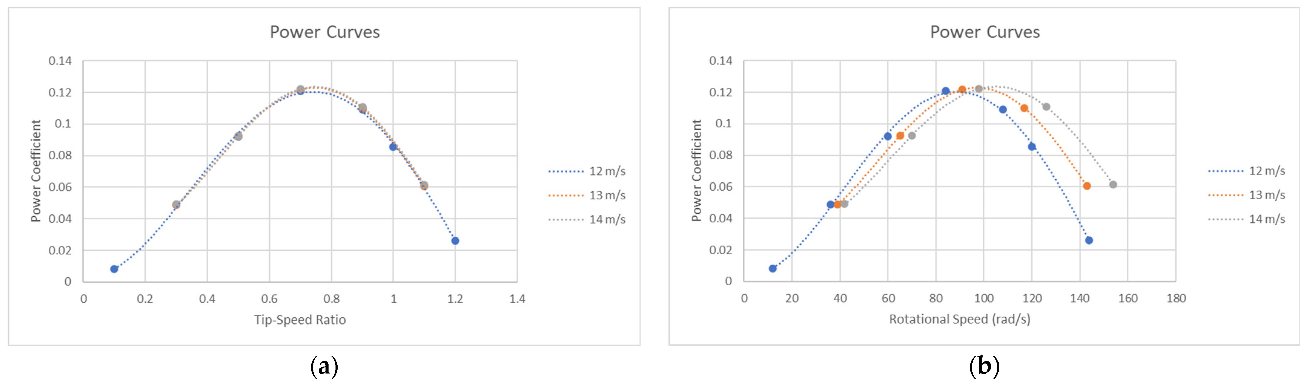
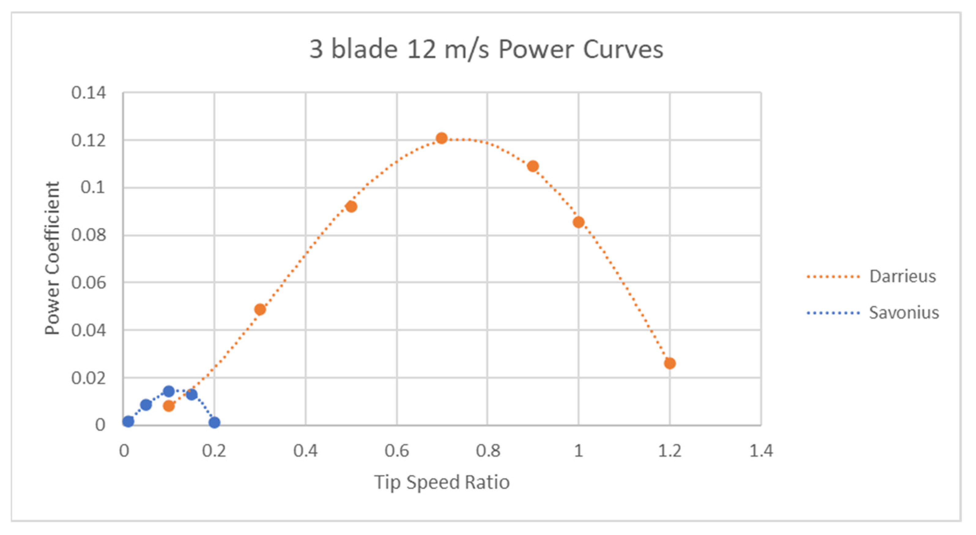
• The best-case scenario efficiency of the VAWT is independent of the wind speed, with the simulation predicting an efficiency of 12.4% at a TSR of 0.7 for the original design.
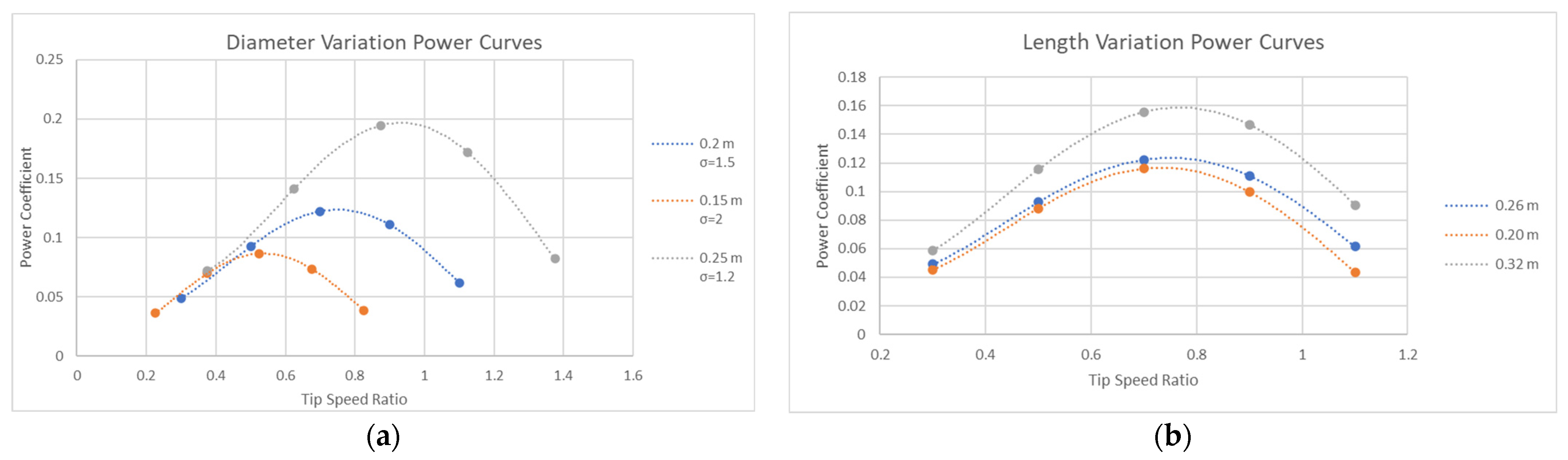
• The current solidity of the design is too high for a Darrieus turbine, with the efficiency increasing as the solidity was lowered by increasing the diameter.
• The design can see an increase in efficiency by increasing the length of the blades.
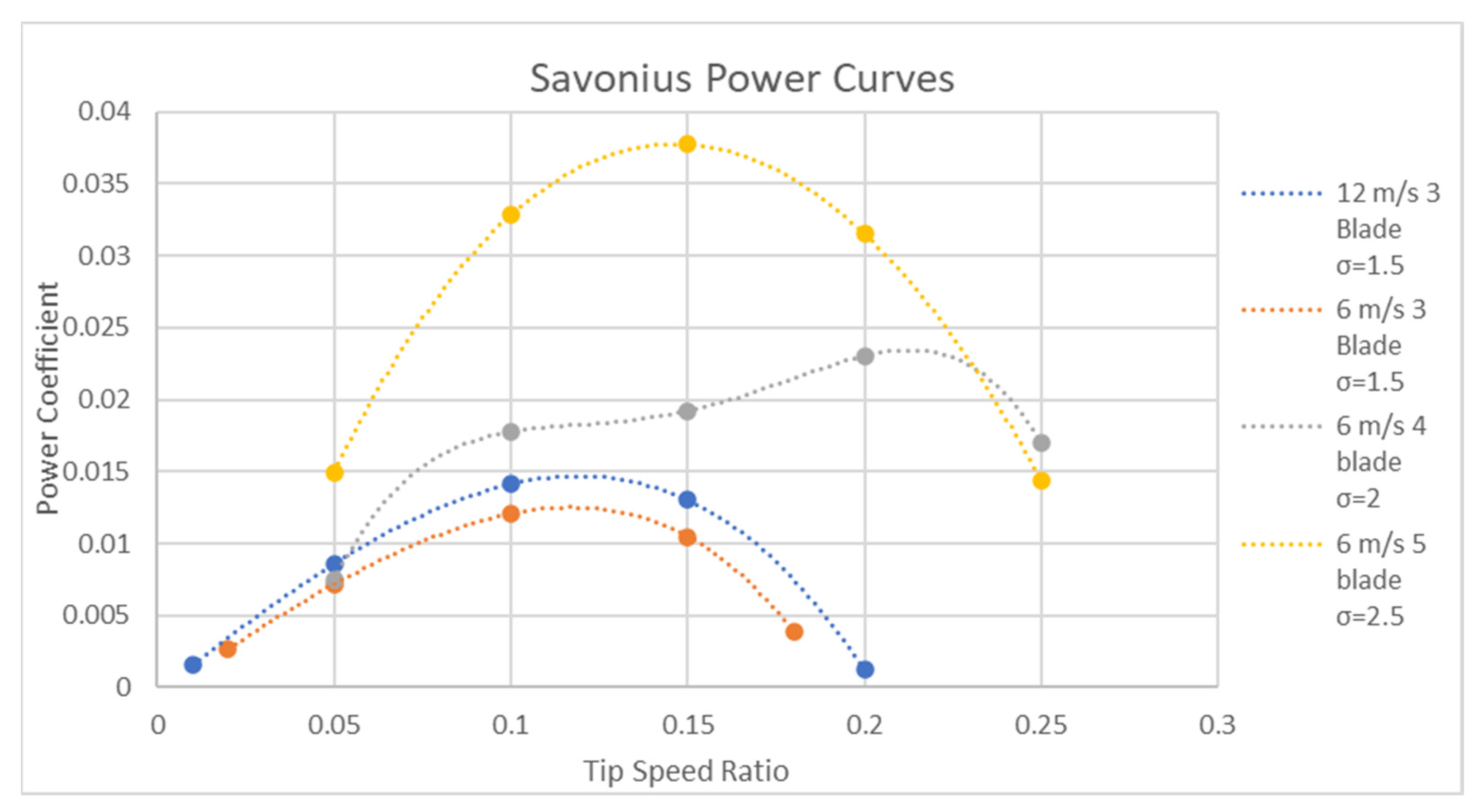
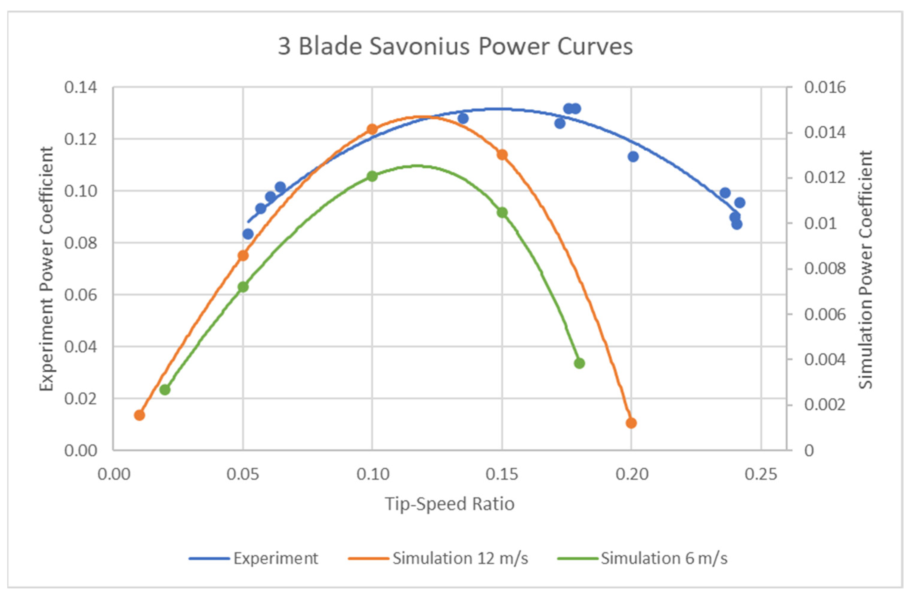
• The simulations showed that the three-blade Savonius design is much less efficient than the Darrieus design for high TSRs; however, the efficiency can be improved by increasing the solidity by increasing the number of blades.
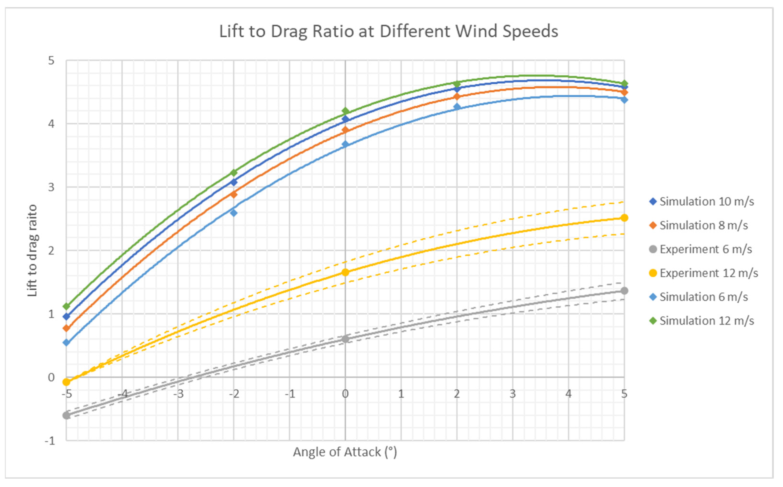
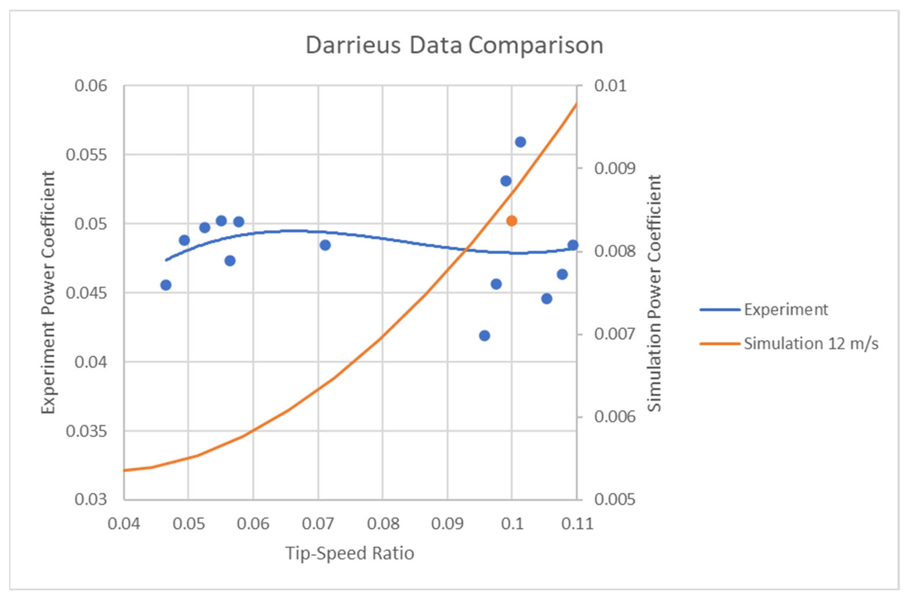
• The experiments showed that the simulations underpredicted the efficiency at low TSRs, with an average of a tenfold increase found.
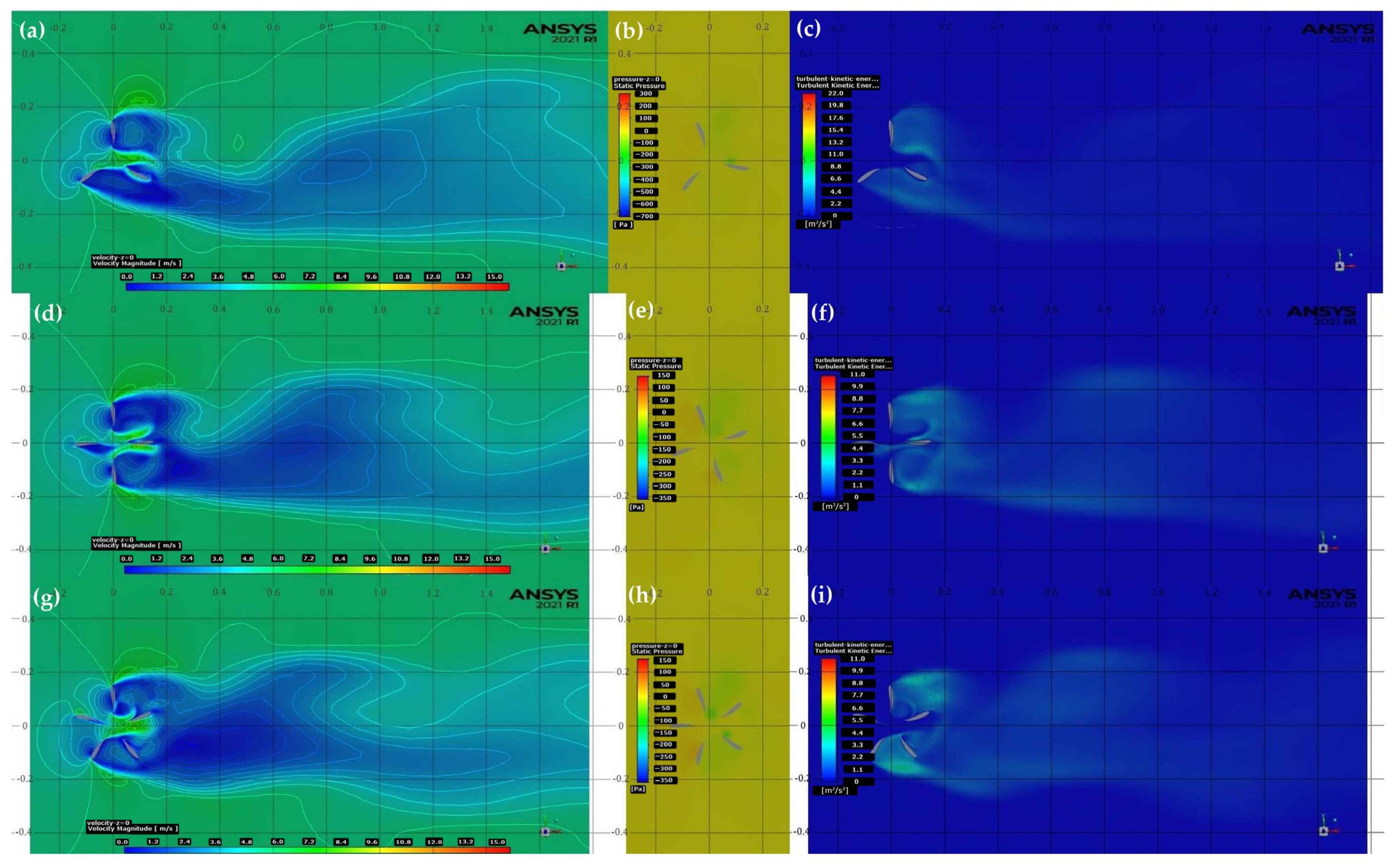
• Increasing the TSR will decrease the wake recovery distance, making the design more suitable for implementation in a wind farm.
• The blade length does not affect the wake recovery distance; however, increasing the diameter, changing to a Savonius design, and increasing the number of blades all increase the wake recovery distance.

Based on the findings and process of this research the following recommendations for future work have been made:

• Due to the large discrepancy in values obtained in the experiment and simulations, further experiments could be performed with models that represent the changes to the design parameters. The main purpose of this would be to determine if the same trends as found in the simulations are found from the experiments to verify whether the simulations have accurately predicted changes in performance.
• A cost performance analysis can be performed with the designs that obtained higher efficiency, with the aim of determining the point where efficiency increases are outweighed by increased costs.
• Simulations can be performed with the full supporting structure of the VAWT. These can then be compared to simulations without the supports and with other support designs, to determine the optimal structure.
• The 3D simulations took a long duration requiring a full day per simulation. Therefore, methods of reducing simulation time can be investigated. These could include the use of Reduced Order Models [14,25], which can significantly reduce the time to obtain a specific set of data.
• Based on the angle of attack of 0° not being optimal for the lift of a single blade, the effect of varying the angle of attack of the blades on the VAWT by small increments could be investigated.
• The effects of the turbine could be investigated to determine how the boundary flow created by the ground will affect the operation of the turbine.

References

1. Franchina, N.; Kouaissah, O.; Persico, G.; Savini, M. Three-Dimensional CFD Simulation and Experimental Assessment of the Performance of a H-Shape Vertical-Axis Wind Turbine at Design and Off-Design Conditions. Int. J. Turbomach. Propuls. Power 2019, 4, 30. [Google Scholar] [CrossRef] [Green Version]
2. Simão Ferreira, C.; van Kuik, G.; van Bussel, G.; Scarano, F. Visualization by PIV of dynamic stall on a vertical axis wind turbine. Exp. Fluids 2009, 46, 97–108. [Google Scholar] [CrossRef] [Green Version]
3. Ebrahimpour, M.; Shafaghat, R.; Alamian, R.; Safdari Shadloo, M. Numerical Investigation of the Savonius Vertical Axis Wind Turbine and Evaluation of the Effect of the Overlap Parameter in Both Horizontal and Vertical Directions on Its Performance. Symmetry 2019, 11, 821. [Google Scholar] [CrossRef] [Green Version]
4. Antar, E.; El Cheikh, A.; Elkhoury, M. A dynamic rotor vertical-axis wind turbine with a blade transitioning capability. Energies 2019, 12, 1446. [Google Scholar] [CrossRef] [Green Version]
5. Hosseini, A.; Goudarzi, N. Design and CFD study of a hybrid vertical-axis wind turbine by employing a combined Bach-type and H-Darrieus rotor systems. Energy Convers. Manag. 2019, 189, 49–59. [Google Scholar] [CrossRef]
6. Durkacz, J.; Islam, S.; Chan, R.; Fong, E.; Gillies, H.; Karnik, A.; Mullan, T. CFD modelling and prototype testing of a Vertical Axis Wind Turbines in planetary cluster formation. Energy Rep. 2021, 7, 119–126. [Google Scholar] [CrossRef]
7. Stout, C.; Islam, S.; White, A.; Arnott, S.; Kollovozi, E.; Shaw, M.; Droubi, G.; Sinha, Y.; Bird, B. Efficiency Improvement of Vertical Axis Wind Turbines with an Upstream Deflector. Energy Procedia 2017, 118, 141–148. [Google Scholar] [CrossRef]
8. Subramanian, A.; Yogesh, S.A.; Sivanandan, H.; Giri, A.; Vasudevan, M.; Mugundhan, V.; Velamati, R.K. Effect of airfoil and solidity on performance of small scale vertical axis wind turbine using three dimensional CFD model. Energy 2017, 133, 179–190. [Google Scholar] [CrossRef]
9. Gao, Q.; Lian, S.; Yan, H. Aerodynamic Performance Analysis of Adaptive Drag-Lift Hybrid Type Vertical Axis Wind Turbine. Energies 2022, 15, 5600. [Google Scholar] [CrossRef]
10. Ahmad, M.; Shahzad, A.; Akram, F.; Ahmad, F.; Shah, S.I.A. Design optimization of Double-Darrieus hybrid vertical axis wind turbine. Ocean Eng. 2022, 254, 111171. [Google Scholar] [CrossRef]
11. Belabes, B.; Paraschivoiu, M. Numerical study of the effect of turbulence intensity on VAWT performance. Energy 2021, 233, 121139. [Google Scholar] [CrossRef]
12. Almohammadi, K.M.; Ingham, D.B.; Ma, L.; Pourkashanian, M. Modeling dynamic stall of a straight blade vertical axis wind turbine. J. Fluids Struct. 2015, 57, 144–158. [Google Scholar] [CrossRef]
13. Wong, K.H.; Chong, W.T.; Poh, S.C.; Shiah, Y.; Sukiman, N.L.; Wang, C. 3D CFD simulation and parametric study of a flat plate deflector for vertical axis wind turbine. Renew. Energy 2018, 129, 32–55. [Google Scholar] [CrossRef]
14. Le Clainche, S.; Ferrer, E. A reduced order model to predict transient flows around straight bladed vertical axis wind turbines. Energies 2018, 11, 566. [Google Scholar] [CrossRef] [Green Version]
15. Alaimo, A.; Esposito, A.; Messineo, A.; Orlando, C.; Tumino, D. 3D CFD Analysis of a Vertical Axis Wind Turbine. Energies 2015, 8, 3013–3033. [Google Scholar] [CrossRef] [Green Version]
16. Lositaño, I.C.M.; Danao, L.A.M. Steady wind performance of a 5 kW three-bladed H-rotor Darrieus Vertical Axis Wind Turbine (VAWT) with cambered tubercle leading edge (TLE) blades. Energy 2019, 175, 278–291. [Google Scholar] [CrossRef]
17. Karimian, S.M.H.; Abdolahifar, A. Performance investigation of a new Darrieus Vertical Axis Wind Turbine. Energy 2020, 191, 116551. [Google Scholar] [CrossRef]
18. Rogowski, K. Numerical studies on two turbulence models and a laminar model for aerodynamics of a vertical-axis wind turbine. J. Mech. Sci. Technol. 2018, 32, 2079–2088. [Google Scholar] [CrossRef]
19. Hand, B.; Cashman, A. Aerodynamic modeling methods for a large-scale vertical axis wind turbine: A comparative study. Renew. Energy 2018, 129, 12–31. [Google Scholar] [CrossRef]
20. Lam, H.F.; Peng, H.Y. Study of wake characteristics of a vertical axis wind turbine by two- and three-dimensional computational fluid dynamics simulations. Renew. Energy 2016, 90, 386–398. [Google Scholar] [CrossRef]
21. Li, Q.; Maeda, T.; Kamada, Y.; Murata, J.; Kawabata, T.; Shimizu, K.; Ogasawara, T.; Nakai, A.; Kasuya, T. Wind tunnel and numerical study of a straight-bladed Vertical Axis Wind Turbine in three-dimensional analysis (Part II: For predicting flow field and performance). Energy 2016, 104, 295–307. [Google Scholar] [CrossRef]
22. Franchina, N.; Persico, G.; Savini, M. 2D-3D Computations of a Vertical Axis Wind Turbine Flow Field: Modeling Issues and Physical Interpretations. Renew. Energy 2019, 136, 1170–1189. [Google Scholar] [CrossRef]
23. Hand, B.; Kelly, G.; Cashman, A. Numerical simulation of a vertical axis wind turbine airfoil experiencing dynamic stall at high Reynolds numbers. Comput. Fluids 2017, 149, 12–30. [Google Scholar] [CrossRef]
24. Trivellato, F.; Raciti Castelli, M. On the Courant–Friedrichs–Lewy criterion of rotating grids in 2D vertical-axis wind turbine analysis. Renew. Energy 2014, 62, 53–62. [Google Scholar] [CrossRef]
25. Tingey, E.B.; Ning, A. Development of a parameterized reduced-order vertical-axis wind turbine wake model. Wind Eng. 2020, 44, 494–508. [Google Scholar] [CrossRef] [Green Version]
26. Siddiqui, M.S.; Durrani, N.; Akhtar, I. Quantification of the effects of geometric approximations on the performance of a vertical axis wind turbine. Renew. Energy 2015, 74, 661–670. [Google Scholar] [CrossRef]
27. He, J.; Jin, X.; Xie, S.; Cao, L.; Wang, Y.; Lin, Y.; Wang, N. CFD modeling of varying complexity for aerodynamic analysis of H-vertical axis wind turbines. Renew. Energy 2020, 145, 2658–2670. [Google Scholar] [CrossRef]
28. Rolland, S.; Newton, W.; Williams, A.J.; Croft, T.N.; Gethin, D.T.; Cross, M. Simulations technique for the design of a vertical axis wind turbine device with experimental validation. Appl. Energy 2013, 111, 1195–1203. [Google Scholar] [CrossRef]
29. Mohamed, M. Impacts of solidity and hybrid system in small wind turbines performance. Energy 2013, 57, 495–504. [Google Scholar] [CrossRef]
30. Wright, L.; Droubi, M.; Islam, S. Computational fluid dynamics simulation for predicting effect of icing on offshore wind turbine blade. In Proceedings of the 13th International Conference on Fluid Control, Measurements and Visualization, Doha, Qatar, 15–18 November 2015; pp. 15–18. [Google Scholar]
Figure 1. Single blade geometry: (a) Viewed from above; (b) Viewed from side; (c) Isometric view.
Energies 16 01144 g001
Figure 2. Darrieus vertical axis wind turbine (VAWT) geometry: (a) Viewed from above; (b) Viewed from side; (c) Isometric view.
Energies 16 01144 g002
Figure 3. Close-up of Savonius turbine with: (a) 3 blades; (b) 4 blades; (c) 5 blades.
Energies 16 01144 g003
Figure 4. Cross-section of 1.4 million element mesh for Darrieus VAWT: (a) Full mesh; (b) Close-up of mesh centre; (c) Close-up of mesh around a blade.
Energies 16 01144 g004
Figure 5. Three-point balance.
Energies 16 01144 g005
Figure 6. VAWT experiment setup.
Energies 16 01144 g006
Figure 7. Single blade lift to drag ratio.
Energies 16 01144 g007
Figure 8. Power curves of unaltered Darrieus VAWT plotted against: (a) Tip-speed ratio (TSR); (b) Rotational speed.
Energies 16 01144 g008
Figure 9. Isometric view of velocity contour for wind speed 14 m/s at TSR of 0.7.
Energies 16 01144 g009
Figure 10. Contours for 14 m/s wind speed of: (a) Velocity at TSR of 0.3; (b) Pressure at TSR of 0.3; (c) Turbulent kinetic energy (TKE) at TSR of 0.3; (d) Velocity at TSR of 0.5; (e) Pressure at TSR of 0.5; (f) TKE at TSR of 0.5; (g) Velocity at TSR of 0.7; (h) Pressure at TSR of 0.7; (i) TKE at TSR of 0.7; (j) Velocity at TSR of 0.9; (k) Pressure at TSR of 0.9; (l) TKE at TSR of 0.9; (m) Velocity at TSR of 1.1; (n) Pressure at TSR of 1.1; (o) TKE at TSR of 1.1.
Energies 16 01144 g010
Figure 11. Contours for 14 m/s wind speed at different stages of rotation of: (a) Velocity at 360°; (b) Pressure at 360°; (c) TKE at 360°; (d) Velocity at 320°; (e) Pressure at 320°; (f) TKE at 320°; (g) Velocity at 280°; (h) Pressure at 280°; (i) TKE at 280°.
Energies 16 01144 g011
Figure 12. Power curves for variation of: (a) Diameter; (b) Blade length/height.
Energies 16 01144 g012
Figure 13. Contours at wind speed 14 m/s, rotational speed 98 rad/s for varied diameters: (a) Velocity at 0.15 m; (b) Pressure at 0.15 m; (c) TKE at 0.15 m; (d) Velocity at 0.20 m; (e) Pressure at 0.20 m; (f) TKE at 0.20 m; (g) Velocity at 0.25 m; (h) Pressure at 0.25 m; (i) TKE at 0.25 m.
Energies 16 01144 g013
Figure 14. Contours at wind speed 14 m/s, rotational speed 98 rad/s for varied blade lengths/heights: (a) Velocity at 0.15 m; (b) Pressure at 0.15 m; (c) TKE at 0.15 m; (d) Velocity at 0.20 m; (e) Pressure at 0.20 m; (f) TKE at 0.20 m; (g) Velocity at 0.25 m; (h) Pressure at 0.25 m; (i) TKE at 0.25 m.
Energies 16 01144 g014
Figure 15. Darrieus and Savonius comparison.
Energies 16 01144 g015
Figure 16. Contours for Savonius three-blade turbine at wind speed 6 m/s of: (a) Velocity at TSR of 0.05; (b) Pressure at TSR of 0.05; (c) TKE at TSR of 0.05; (d) Velocity at TSR of 0.10; (e) Pressure at TSR of 0.10; (f) TKE at TSR of 0.10; (g) Velocity at TSR of 0.20; (h) Pressure at TSR of 0.20; (i) TKE at TSR of 0.20.
Energies 16 01144 g016
Figure 17. Savonius design comparison.
Energies 16 01144 g017
Figure 18. Contours at wind speed 6 m/s, TSR 0.1, for Savonius with varied number of blades: (a) Velocity with 3 blades; (b) Pressure with 3 blades; (c) TKE with 3 blades; (d) Velocity with 4 blades; (e) Pressure with 4 blades; (f) TKE with 4 blades; (g) Velocity with 5 blades; (h) Pressure with 5 blades; (i) TKE with 5 blades.
Energies 16 01144 g018
Figure 19. Single blade lift-to-drag ratios with simulation and experiment data, with ±10% error lines for experimental data, represented by dashed lines.
Energies 16 01144 g019
Figure 20. Unaltered Darrieus turbine data comparison.
Energies 16 01144 g020
Figure 21. Velocity contour at 12 m/s wind speed and TSR of 0.1, with enlarged legend.
Energies 16 01144 g021
Figure 22. Smoke flow: (a) From the inlet; (b) Around the returning side.
Energies 16 01144 g022
Figure 23. Velocity streamlines at wind speed 14 m/s and TSR of 0.1.
Energies 16 01144 g023
Figure 24. Three-blade Savonius simulation and experiment comparison.
Energies 16 01144 g024