Data-Driven Dynamic Stability Assessment in Large-Scale Power Grid Based on Deep Transfer Learning

Abstract

For data-driven dynamic stability assessment (DSA) in modern power grids, DSA models generally have to be learned from scratch when faced with new grids, resulting in high offline computational costs. To tackle this undesirable yet often overlooked problem, this work develops a light-weight framework for DSA-oriented stability knowledge transfer from off-the-shelf test systems to practical power grids. A scale-free system feature learner is proposed to characterize system-wide features of various systems in a unified manner. Given a real-world power grid for DSA, selective stability knowledge transfer is intelligently carried out by comparing system similarities between it and the available test systems. Afterward, DSA model fine-tuning is performed to make the transferred knowledge adapt well to practical DSA contexts. Numerical test results on a realistic system, i.e., the provincial GD Power Grid in China, verify the effectiveness of the proposed framework.

1. Introduction

The recent advancement of machine learning (ML) technologies, especially deep learning (DL) methods, has opened a new door to solving various challenging stability problems in bulk power systems [1] and microgrids [2] from a data-driven perspective [3,4,5]. Taking online dynamic stability assessment (DSA), for example, with massive measurement data acquired by phasor measurement units (PMUs) [1,6], many ML-/DL-based efforts have been made in the research community to achieve rapid and reliable online DSA in smart grids. In particular, some inspiring DSA-oriented data-driven schemes have been proposed in the last three years [7,8,9,10,11,12,13], which shapes the state-of-the-art in the area of data-driven power system DSA. These representative studies are briefly reviewed in the following.

In [7], a convolutional neural network (CNN)-based learning machine is presented to perform online transient stability assessment (TSA). With a well-designed two-level learning mechanism, this machine is able to implement both quantitative and qualitative TSA with high reliability. A data-driven TSA scheme is realized in [8] by combining a denoising stacked autoencoder (AE) with a voting ensemble classifier. With this combination, the TSA scheme can effectively reduce the dimensionality of the original feature space while preserving the maximum information for online decision-making. A supervised dictionary learning method with desirable accuracy and adaptability is proposed in [9] to carry out online TSA. It exhibits superior TSA performances over existing methods such as singular value decomposition, though at the cost of compromising the online decision-making speed. In [10], a recurrent convolutional neural network that combines CNN with the long short-term memory (LSTM) algorithm is designed to address both TSA and short-term voltage stability assessment. With the consideration of various defective conditions in practice (e.g., TSA implementation time delays and practical measurement noises), the proposed learning network has shown to be highly promising in practical systems. By learning from pre-fault and fault-on measurements of a given system, a fast TSA scheme is presented in [11], which can issue the online TSA results almost immediately after fault clearance. In [12], a dual-stream CNN-based learning scheme is utilized to predict the key eigenvalues of the monitored system for low-frequency oscillation detection. With high-precision eigenvalue prediction achieved, this scheme can provide valuable information to support the implementation of low-frequency oscillation damping control in practice. Taking into account the reality gap between the simulation model for offline learning data generation and the practical grid for online monitoring, a generative adversarial network-enabled learning approach is developed in [13] to produce high-fidelity learning data to support the reliable realization of data-driven DSA in practice.

Overall, the above-reviewed studies [7,8,9,10,11,12,13] have exhibited high potential in addressing the DSA problem from the data-driven perspective. However, they have two non-trivial defects when applied to practical large-scale power grids. First, the input sizes of the DSA models in these studies generally depend on the scale of the specific grids. In this regard, the input dimensionality would become very high when faced with an extremely large system involving numerous buses and transmission lines. Consequently, this would cause the curse of dimensionality, affecting the scalability of these studies in practical large systems. Second, their data-driven DSA models generally need to be trained from scratch when applied to new systems, introducing very high computational burdens into time-domain (TD) simulation-based offline learning data preparation. Although this does not necessarily impair the online efficiency of DSA model application, it could limit the applicability of data-driven DSA methods in practice. For example, given the China Southern Power Grid (with more than 10,000 buses across five provinces in South China) for data-driven DSA implementation, the dimensionality of the learning inputs can be as large as tens of thousands. Besides, if 15,000 transient cases need to be generated for offline learning, according to the authors’ empirical tests, it takes about five days to generate such a large-size dataset via batch TD simulations. Such a high computational cost would make it impossible to efficiently implement online model retraining/updating, which could have helped enhance the data-driven model’s adaptability to unforeseen operation changes during online monitoring.

With recent advances in transfer learning (TL), concentrating on knowledge transfer between different yet related learning tasks or domains [14], it is viable to transfer learned stability knowledge to new scenarios/systems for data-driven DSA in smart grids. Recently, several inspiring TL-based DSA methods have been reported in the literature. In particular, a TL scheme is proposed in [15] to assess power grid security under multiple unseen faults using the data-driven surrogate model learned from a single transient fault. In [16], based on instance transfer learning, the knowledge of power system dynamics w.r.t. transient fault-affected areas is incorporated into TSA model training to improve the reliability of online TSA against specific contingencies. However, to the best of the authors’ knowledge, none of the existing studies have paid attention to the issue of how to transfer stability knowledge between different power systems for efficient DSA implementation.

In fact, given two power systems with different scales and complexities yet similar dynamic behaviors, one may first learn stability knowledge from the relatively small one (denoted as the source system) and then transfer it to the large one (denoted as the target system) via TL. By doing so, the DSA model to be derived for the large system can be efficiently initialized with the transferred knowledge and finely tuned with a small number of representative learning cases generated from the large system. With no need for learning from scratch again, the number of learning cases for DSA model derivation in the target system can be largely reduced. This would significantly alleviate the above-mentioned heavy computational burden of offline case generation and DSA model training in the large target system, thereby making data-driven DSA more tractable and scalable in practical large-scale grids. However, to realize such a TL-based light-weight DSA scheme, two challenging yet crucial problems need to be addressed: (1) With structures and dynamic characteristics varying from system to system, how to appropriately choose a small source system to implement TL for the target system in practice is the cornerstone of effective knowledge transfer. (2) To transfer knowledge between systems with different scales and structures, a compatible TL scheme characterizing different systems’ stability features in a unified fashion should be carefully designed, so as to make the TL procedure independent of system scales and thus overcome the curse of dimensionality in practical large systems.

To cope with the above challenging issues, this work develops an intelligent stability knowledge transfer framework to efficiently implement data-driven DSA in practical large-scale power grids. Focusing on TSA, a scale-free system feature learner is proposed to abstract the transient characteristics of individual systems with arbitrary scales and structures in a unified manner. Based on this learner, a series of typical small test systems are taken as the source candidates for compatible stability feature learning and stability knowledge preparation. For a target-practical grid, selective stability knowledge transfer is intelligently implemented by borrowing TSA models from test systems highly resembling the target grid, and TSA model fine-tuning is carried out using a small number of cases collected from the grid. The major contributions of this work lie in two folds:

• This work develops a novel TL framework to carry out data-driven DSA for practical large power grids in a light-weight way. With the offline computational burden of DSA model derivation largely eased, it can help enhance existing data-driven DSA solutions’ applicability in practice.
• A scale-free system feature learner is proposed for the first time to abstract power system dynamic features from massive operation scenarios in a unified manner, regardless of the scale and complexity of the given system.

The rest of the paper is organized as follows. Section 2 presents the scale-free system feature learner for system-wide dynamic feature description. Based on this learner, Section 3 describes the proposed TL framework for efficient DSA implementation in practical large power grids. After that, case studies are carried out in Section 4 to examine the efficacy of the proposed framework. Finally, Section 5 concludes the whole work.

2. Scale-Free System Feature Learner

Before detailing the main methodology, a fully data-driven system feature learner with no need for any power network parameters is proposed to characterize system-wide features of diverse systems in a unified way. To sufficiently capture system dynamic features in various transient scenarios, this learner is devised to learn from transient trajectories of numerous transient cases. For a specific system, by acquiring raw responsive time series (TS) data from n transient cases, a transient case set is first formed as

$$\mathcal{S}=\left\{({\mathit{x}}_i,y_i)\left|{\mathit{x}}_i=\left\{{\mathit{V}}_i,{\mathbf{\theta }}_i,{\Delta \mathit{f}}_i\right\},\mathrm{for}1\le i\le n\right.\right\}$$

(1)

where $({\mathit{x}}_i,y_i)$ denotes the pair of multi-variable TS trajectories and binary stability status of case i ($1\le i\le n$). In particular, assuming m major generators in the system are deployed with PMUs, ${\mathit{x}}_i$ is acquired from the corresponding generator buses. In this paper, three types of variables that can be directly measured by PMUs at generator buses, i.e., bus voltage magnitudes (${\mathit{V}}_i$), relative bus voltage angles (${\mathbf{\theta }}_i$, with reference to a given generator bus) and bus frequency deviations (${\Delta \mathit{f}}_i$) are sequentially collected to form $3m$-variable TS trajectories, i.e., ${\mathit{x}}_i$. The reason why these variables are chosen is briefly explained below. In a specific system, rotor angle swings of individual generators are the most straightforward indicators of system transient stability. However, as demonstrated in existing TSA studies [10,17,18,19], generator bus voltages (including both voltage magnitudes and phases) evolving much faster than rotor angles can be employed to predict transient stability more efficiently. Besides, as the frequency deviations of generator buses are related to the speeds of generators, they have been verified to be informative variables as well for the prediction of system transient stability [18,20]. Taking into additional account the factor that all the variables should be conveniently measured by PMU devices to support the implementation of a fully data-driven TSA scheme in practice, this paper thus selects the data of $\{V,\theta ,\Delta f\}$ acquired from individual generator buses as the major input variables for data-driven TSA.

For the sake of helping carry out online TSA with a high response speed, a short observation time window $T_{\mathrm{win}}$ ($\left|T_{\mathrm{win}}\right|$ < 1 s) is utilized for acquiring TS data of $\{V,\theta ,\Delta f\}$. In particular, it is set to start from the instant of fault occurrence and end at early post-fault stages. The stability status of case i, i.e., $y_i$, is determined by the following widely-used stability criterion [21]:

$$y_i=\{\begin{array}{cc}\hfill 1\mathrm{if}{\eta }_i>0& \left(\mathrm{stable}\right)\\ 0\mathrm{else}\hfill & \hspace{1em}\left(\mathrm{unstable}\right)\end{array},\mathrm{for}{\eta }_i=\frac{{360}^{\mathrm{o}}-{\left|\Delta \delta \right|}_{max i}}{{360}^{\mathrm{o}}+{\left|\Delta \delta \right|}_{max i}}$$

(2)

where $|\Delta {\delta |}_{max i}$ is the maximum absolute value of rotor angle differences between any two generators during the transient process of case i.

Taking the $3m$-variable TS trajectories ${\mathit{x}}_i$ as both the input and output, the feature learner is designed to learn the transient features of the system in an unsupervised way. Specifically, it is realized in the form of a sequential AE by combining the LSTM network with the AE algorithm [22], as illustrated in Figure 1.

With both its encoder and decoder modules consisting of two sequential LSTM units, the learner first learns the temporal evolution of multiple TS trajectories and encodes them with compact vectors. Then, it decodes these vectors to reconstruct the original trajectories as precisely as possible. Its overall learning objective is given by

$$min{\mathcal{L}}_1=min\sqrt{\frac{1}{n}{\sum }_{i=1}^n{\left|{\mathit{x}}_i-{\mathit{x}}_i^{{}^{\prime }}\right|}^2}$$

(3)

where ${\mathcal{L}}_1$ is the loss function, and ${\mathit{x}}_i^{{}^{\prime }}$ is the $3m$-variable TS trajectories reconstructed by the decoder. In essence, the hidden states after encoding represent the critical features and characteristics automatically learned from the system. Hence, the corresponding encoded vectors are extracted and regarded as the primary system features. Supposing there are $m^{\prime }$ hidden neurons after the encoder module for feature encoding, the original $3m$-variable TS trajectories of $\{{\mathit{V}}_i,{\mathbf{\theta }}_i,{\Delta \mathit{f}}_i\}$ are concisely described by three featured vectors, which are briefly denoted by $\{{\mathit{X}}_{i1},{\mathit{X}}_{i2},{\mathit{X}}_{i3}\}$. Note that the length of such featured vectors is determined by the number of neurons in the sequential AE, i.e., $m^{\prime }$, rather than the initial dimensionality of ${\mathit{x}}_i$. Since no power network model or parameter is involved in this learner, it has a desirable nonparametric feature.

This sequential AE-based feature learner can bring multiple benefits into the whole TL-based TSA framework. With its help, the original bulky TS dataset can be transformed into a light-weight featured dataset. This transformation results in automatic dimensionality reduction and learning efficiency improvement for subsequent TSA model training. More importantly, when applied to systems with different scales and network structures, it can serve as a unified data preprocessing tool to yield featured datasets with the same dimensionality. This makes it possible to quantify the similarities between heterogeneous systems, which lays a solid foundation for the implementation of subsequent similarity-based stability knowledge transfer.

3. Proposed Framework

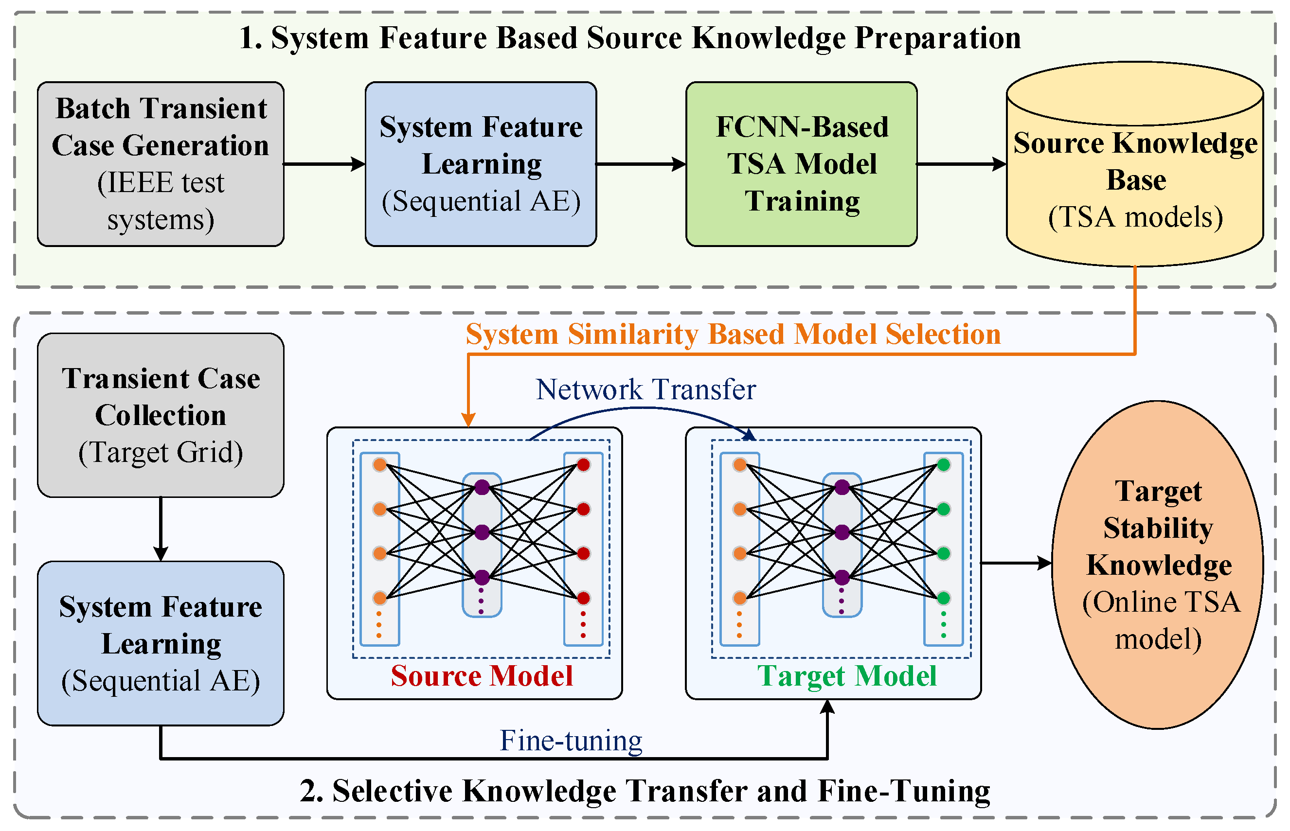
The TL framework for practical TSA is presented in this section, as shown in Figure 2. Its implementation includes two phases: (1) With transient case sets generated from small IEEE test systems, the fully convolutional neural network (FCNN) is employed to train a group of TSA models, which form a source knowledge base for subsequent TL. (2) The TSA model whose original test system shares high similarities with the target large system to be monitored in practice is selected for knowledge transfer, and a small group of learning cases collected from the target system are fed into it for fine-tuning.

3.1. System Feature Based Source Knowledge Preparation

With K typical IEEE test systems taken as source systems for stability knowledge preparation, batch transient case generation is first carried out on them via TD simulations. For each test system, a transient case set is collected from the simulation results and further converted to a featured dataset using the above feature learner. As the FCNN algorithm has been demonstrated to outperform conventional TS learning methods on various benchmark TS datasets in the ML community [23], it is employed as the basic learning algorithm for source TSA model training. The FCNN used in this work includes a three-channel input layer (corresponding to vectorized features ${\mathit{X}}_{i1},{\mathit{X}}_{i2}$ and ${\mathit{X}}_{i3}$), three stacked convolutional layers and a fully connected softmax layer. Taking the binary stability status of the system as the output, the FCNN is trained by minimizing the following cross-entropy loss function:

$$min{\mathcal{L}}_2=min\sum _{i=1}^n\left[-y_i{log}_2{\overline{y}}_i-(1-y_i){log}_2(1-{\overline{y}}_i)\right]$$

(4)

where ${\overline{y}}_i$ and $y_i$ are the predicted value (output of the softmax layer) and the true class label of case i for ${\overline{y}}_i\in [0,1]$ and $y_i\in \{0,1\}$ ($0\to$ unstable, $1\to$ stable). Given a threshold $\epsilon$, the binary stability prediction, denoted by ${\widehat{y}}_i$, can be made via the following rule:

$${\widehat{y}}_i=\{\begin{array}{cc}\hfill 1\mathrm{for}{\overline{y}}_i>\epsilon & \left(\mathrm{stable}\right)\\ 0\mathrm{otherwise}\hfill & \hspace{1em}\left(\mathrm{unstable}\right)\end{array}$$

(5)

Based on FCNN training, K TSA models are derived from the K test systems. In fact, such TSA models represent key stability knowledge of respective test systems for TSA. They are gathered to form a source stability knowledge base, which is readily available for TL application in the next phase.

3.2. Selective Knowledge Transfer and Fine-Tuning

For a target practical system in need of online TSA, the recent historical transient cases are first collected from system operation records. Alternatively, based on the current operating condition and presumed contingencies of the system, TD simulations can be carried out to further supplement transient cases. With the emphasis on alleviating the heavy computational burden related to offline case preparation, the number of simulated cases is assumed to be somewhat small. All the historical/simulated cases are gathered as a learning case set for TL implementation. System feature learning is then conducted to extract system-wide features from all the learning cases. Afterward, a TSA model is borrowed from the previous stability knowledge base and finely tuned with the learning cases to generalize to practical TSA contexts. The key issue here is how to select an appropriate source TSA model. This task is fulfilled by introducing a system dissimilarity measure.

Inspired by multiple TS dataset comparisons in [24], the system dissimilarity measure is computed by averaging featured datasets in different systems and comparing their averaged profiles. Instead of simply averaging encoded vectors over all the cases, the powerful dynamic-time-warping barycenter averaging (DBA) algorithm [25,26] is adopted to estimate the averaged profiles for the source and target systems. Taking a certain source system for instance, based on DBA, two groups of averaged profiles, denoted as ${\mathcal{X}}_s=\{{\overline{\mathit{X}}}_{s1},{\overline{\mathit{X}}}_{s2},{\overline{\mathit{X}}}_{s3}\}$ and ${\mathcal{X}}_u=\{{\overline{\mathit{X}}}_{u1},{\overline{\mathit{X}}}_{u2},{\overline{\mathit{X}}}_{u3}\}$, are abstracted from the featured vectors of all the stable and unstable cases, respectively. For the detailed DBA procedure, interested readers may refer to [25,26]. Similarly, two groups of averaged profiles ${\mathcal{X}}_s^{{}^{\prime }}$ and ${\mathcal{X}}_u^{{}^{\prime }}$ are extracted from the learning cases of the target system. The dissimilarity between the source and target systems is defined as

$$D_{\mathrm{sys}}=\underset{v\in \{s,u\}}{min}D\left({\mathcal{X}}_v,{\mathcal{X}}_v^{{}^{\prime }}\right)$$

(6)

where $D({\mathcal{X}}_v,{\mathcal{X}}_v^{{}^{\prime }})$ is the distance between the averaged profiles of stable/unstable cases. Specifically, it is calculated by

$$D({\mathcal{X}}_v,{\mathcal{X}}_v^{{}^{\prime }})=\sqrt{{\sum }_{i=1}^3{\left({\overline{\mathit{X}}}_{v,i}-{\overline{\mathit{X}}}_{v,i}^{{}^{\prime }}\right)}^2},\mathrm{for}v\in \{s,u\}$$

(7)

Based on (6), all the source systems involved in the first phase are compared with the target system. For those source systems with relatively small dissimilarities to the target system, their TSA models can be selected for stability knowledge transfer. Concretely, the structure and parameters of the selected model are directly copied to form the initial TSA model for the target system. Since both the source and target systems involve the same sizes of FCNN inputs (three-channel vectors) and outputs (two-class labels), no additional neural network modification is needed. After that, the featured dataset obtained from the learning cases of the target system is fed into this model for fine-tuning. By doing so, the TSA model is able to extrapolate well to the target system.

3.3. Online TSA Implementation

With a well-trained TSA model, when a transient fault occurs in the target system, the fault-on and post-fault TS data of {$V,\theta ,\Delta f$} are acquired by PMUs deployed at individual generator buses. These real-time measurements are collected as a measured case, which is then fed into the TSA model for transient stability prediction. The TSA model then issues the stability prediction results, inferring if the system can maintain transient stability. If so, continuous online monitoring would be carried out by sliding the observation time window. Otherwise, alerting signals would be activated to alarm system operators that control actions should be taken as soon as possible to save the system from potential instability.

To evaluate the online TSA performances in a comprehensive manner, three performance metrics, i.e., misdetection rate, false-alarm rate and accuracy [7], are introduced in this paper:

$$Mis=N_{\mathrm{fs}}/N_t\times 100\%$$

(8)

$$Fal=N_{\mathrm{fu}}/N_t\times 100\%$$

(9)

$$Acc=\left(N_t-N_{\mathrm{fu}}-N_{\mathrm{fs}}\right)/N_t\times 100\%$$

(10)

where $N_t$ is the total number of transient cases for online testing, $N_{\mathrm{fs}}$ is the number of unstable cases wrongly classified as stable; $N_{\mathrm{fu}}$ are the number of stable cases falsely alarmed as unstable.

4. Case Study

4.1. Simulation Set-Up and Case Generation

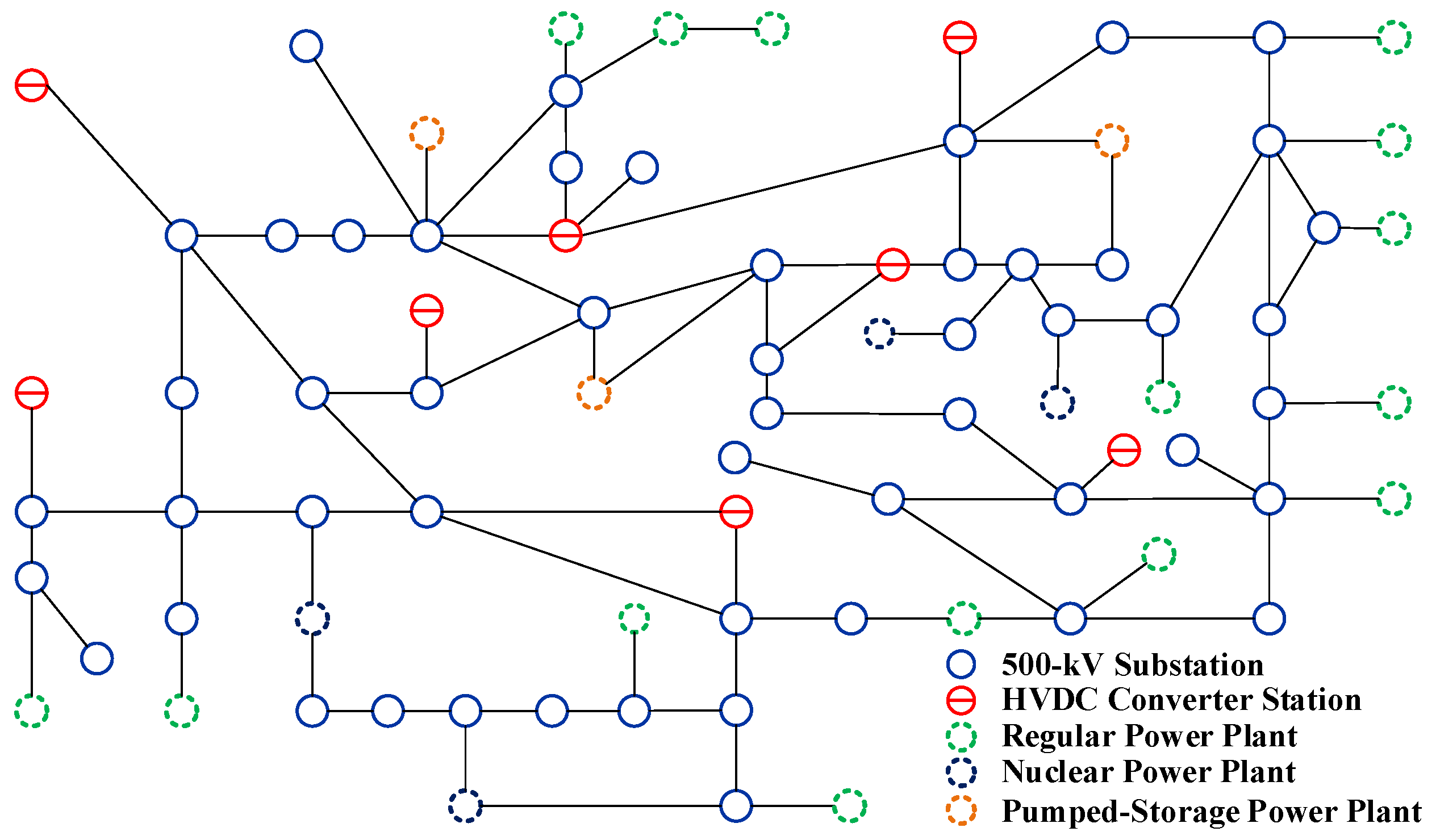
The realistic 2417-bus GD Power Grid (GDPG) in China [7,27] was taken as the target system to verify the performances of the proposed framework. The primary structure of GDPG is illustrated in Figure 3. Based on PSD-BPA, a commercial power system simulation package widely used in China, 300 transient cases were generated from the numerical simulation model of GDPG by considering the recent operating conditions of the system and some representative transient contingencies. These cases were integrated as a small learning case set to support TL implementation in GDPG. For online TSA performance validation, 3000 unseen transient cases with various new operating conditions and transient faults not covered by the initial 300 ones were generated to simulate online testing cases in GDPG. Five typical IEEE test systems, i.e., IEEE 9/14/39/118/162-bus systems, were chosen to build the source knowledge base. Batch TD simulations were conducted in PSD-BPA to generate transient case sets for these test systems. In each test system, 80% of the cases were randomly chosen for source TSA model training, while the remaining 20% for learning performance validation. Since a dedicated validation dataset was provided here for performance testing in each of the test systems, no additional cross validation was introduced into learning performance verification in the sequel.

The length of the observation time window for PMU data acquisition was set to $|T_{\mathrm{win}}|=$ 0.5 s for all systems. The PMU data reporting rate was specified as 100 Hz and 120 Hz for GDPG (with 50-Hz nominal frequency) and the remaining IEEE test systems (with 60-Hz nominal frequency), respectively. All the systems shared the same DL structures and parameter settings. As for the sequential AE-based feature learner, the numbers of neurons of the four LSTM-based encoding and decoding layers were specified as 200, 100, 100, and 200, respectively. With these settings, the length of featured vectors in individual featured datasets turns out to be $m^{\prime }$ = 100. For the hyperparameters of FCNN, the numbers of filters in the three convolutional layers were set to 128, 256, and 128, respectively, with kernel sizes of 8, 5, and 3. In the procedure of offline learning, a widely-used stochastic gradient descent (SGD)-based optimization algorithm called Adam [28] was utilized for DL model training. The learning rate of the Adam optimizer was set to a default value of 0.001. With the mini-batch size specified as 128, mini-batch gradient descent was introduced to help the learning procedure converge in a robust yet efficient manner. All the DL-related computations were implemented in Python 3.6 with the support of the Keras library. The calculations were conducted on a PC configured with a 3.60-GHz Intel Core i7-7700 CPU and an NVIDIA GTX-1080 GPU. As for binary transient stability classification, in order to make TSA decisions with no bias, the threshold in (5) was designated as $\epsilon =$ 0.5.

4.2. Comprehensive Performance Verification

To illustrate the effect of sequential AE-based learning, the root mean square errors (RMSEs) of TS reconstruction on both the training and validation sets were calculated for each of the IEEE test systems. Meanwhile, all the learning and unseen cases generated from GDPG were taken for RMSE estimation. As shown in Figure 4, the sequential AE is able to reliably reconstruct the TS trajectories for all the systems, with the overall RMSE kept below 0.035 pu. This implies that the sequential AE-based system feature learner can capture the critical dynamic features from individual systems with different scales and structures, thereby enabling dimensionality reduction and effective system dissimilarity quantification.

Based on the FCNN algorithm, five TSA models were derived from the five IEEE test systems. Their learning performances on respective validation cases are summarized in

Table 1. Learning Performances of Source TSA Models (with Validation Datasets).

Source System	${\mathit{N}}_{\mathbf{case}}$	$\mathit{Mis}$/%	$\mathit{Fal}$/%	$\mathit{Acc}$/%
IEEE 9	960	0	0	100
IEEE 14	1280	0	0	100
IEEE 39	1920	0	0.26	99.74
IEEE 118	3600	0	0	100
IEEE 162	4800	0.10	0.10	99.80

Note 1: The second column denotes the total number of training and validation cases generated for each test system.

. Obviously, all the TSA models achieve excellent learning performances, with the overall accuracy remaining above 99.5%.

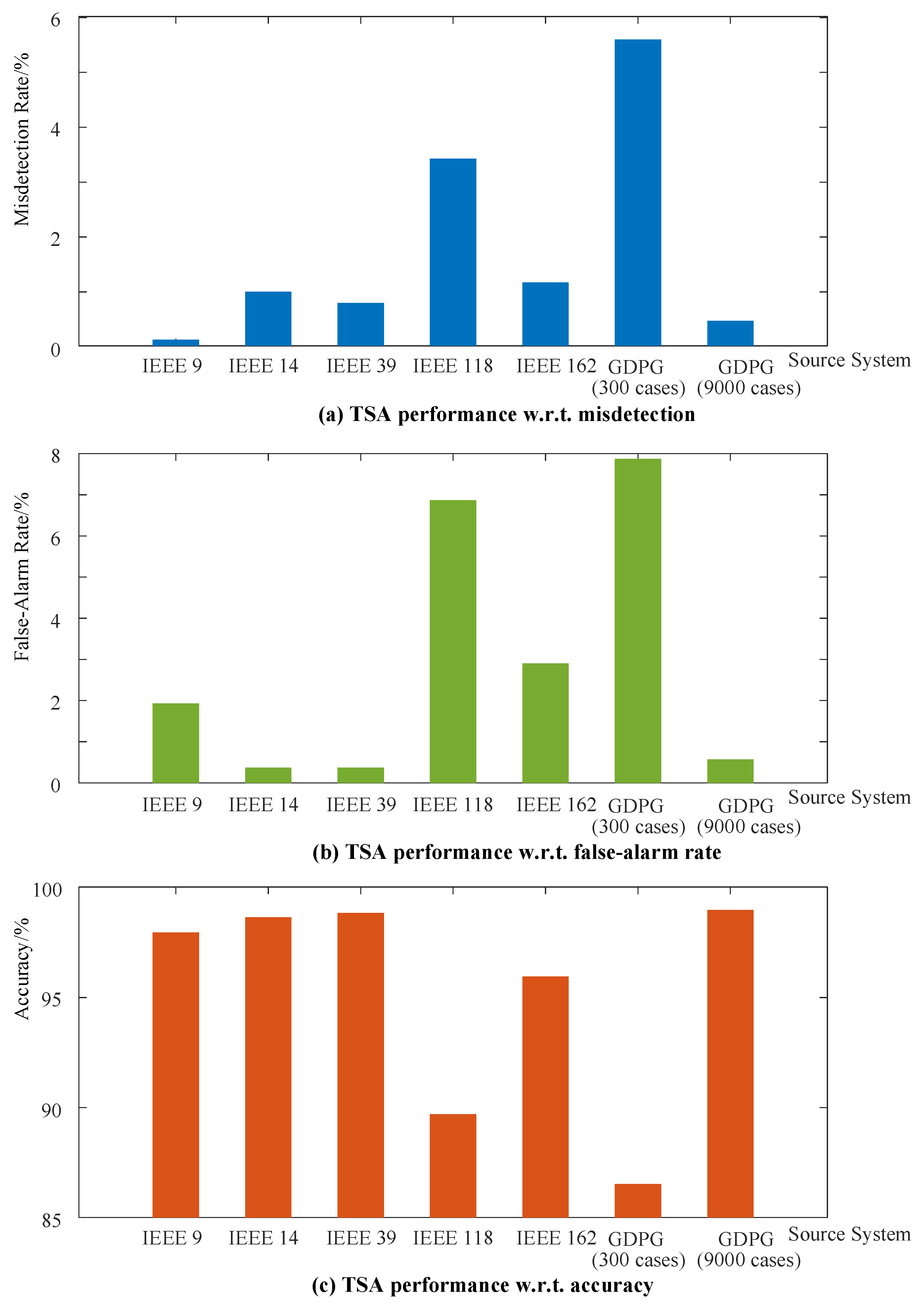
All of the five TSA models were then finely tuned with the 300 learning cases obtained from GDPG, and their tuned versions were further applied to online TSA in GDPG. For comparison, a TSA model was trained from scratch merely using the 300 learning cases. Besides, following the conventional data-driven TSA paradigm without TL [7], another TSA model was directly trained with a large number of learning cases generated from GDPG. Specifically, by considering a wide variety of operating conditions and transient events in GDPG, 9000 learning cases covering massive transient scenarios were produced via batch TD simulations to train this TSA model. 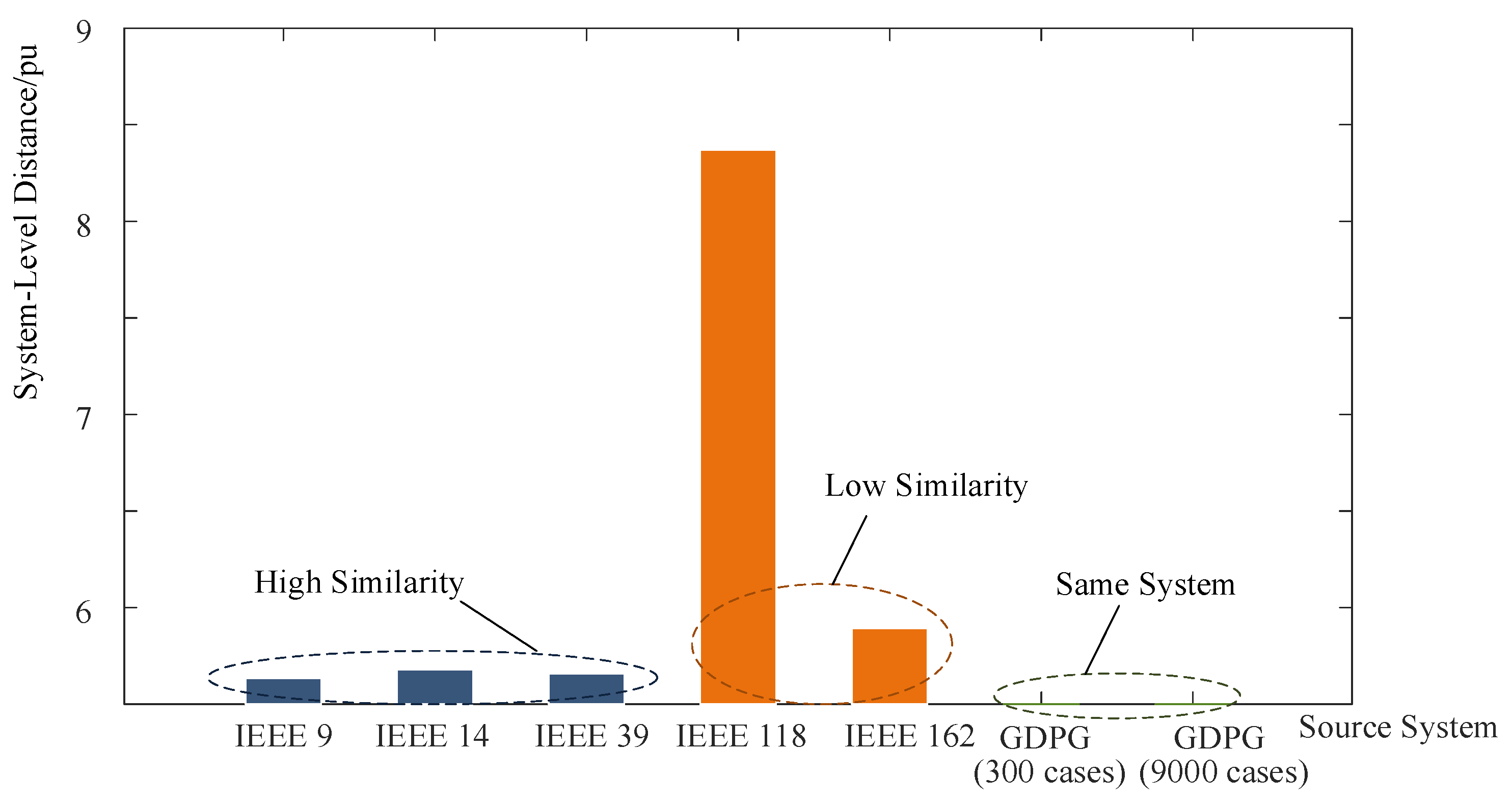All of these experiments resulted in seven TSA models, and their performances on the 3000 unseen cases are presented in Figure 5. Note that, for the last two TSA models directly trained with cases generated from GDPG, no TL is involved, and the trained TSA models were readily applied to online tests. Besides, the source systems corresponding to these seven TSA models were compared with the target GDPG, and their system-level distances based on (7) are illustrated in Figure 6.

Clearly, compared with the TSA model learned from the small 300-case dataset, the other TL-based models enhance online TSA performances significantly. In particular, for the three test systems highly resembling GDPG, i.e., IEEE 9/14/39-bus systems, their well-tuned TSA models achieve highly accurate online TSA in GDPG, with a total accuracy of more than 97.5%. This reveals that the proposed TL framework is able to effectively extend knowledge learned from small test systems to a practical grid for TSA performance enhancement. Note that the TSA models borrowed from the IEEE 14/39-bus systems are almost competitive with that directly derived from the 9000 learning cases in GDPG. This reveals that desirable TSA performances can be intelligently achieved in a TL-based lightweight manner, with no need for generating numerous cases and learning from scratch. As will be shown in the sequel, this would largely improve the offline computational efficiency. Comparatively speaking, the IEEE 118/162-bus systems with lower similarities have a smaller improvement in TSA accuracy, which indicates the efficacy of the system similarity-based model selection for knowledge transfer.

Nonetheless, it is noticed that the IEEE 9-bus system with the highest similarity to GDPG does not contribute to the best TL result. Instead, the IEEE 39-bus system with a bit lower similarity leads to the highest TL performance. This is perhaps because the IEEE 9-bus system has a relatively small dataset (768 cases) for source model training, thereby being difficult to adapt to a wide range of unexpected scenarios in the practical grid. In this regard, the test systems with both sufficient knowledge learned from a large number of scenarios and a relatively high similarity to the practical grid would be a more suitable choice for stability knowledge transfer. Hence, the IEEE 39-bus system is finally selected as the source system for TSA-oriented knowledge transfer toward GDPG.

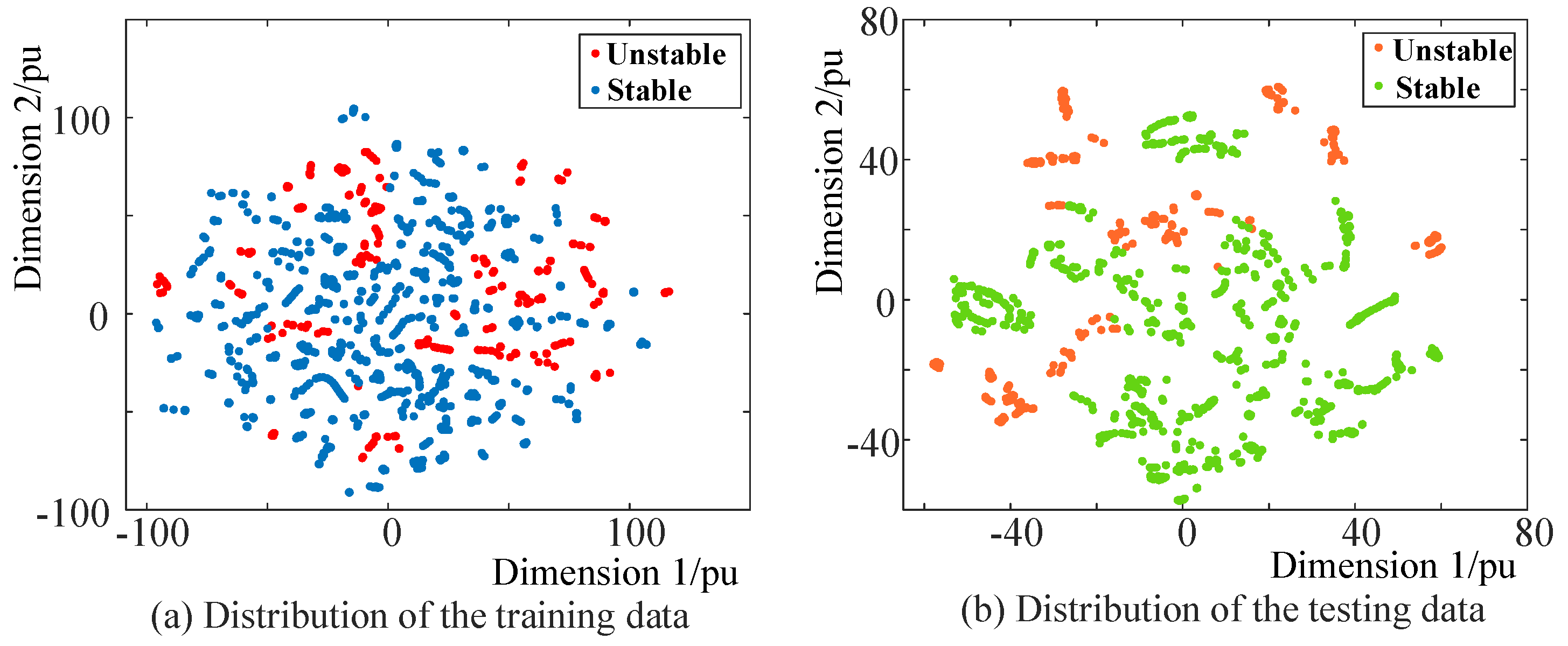
To analyze the data characteristics of the cases generated in the source (IEEE 39-bus) and target (GDPG) system, the t-distributed stochastic neighbor embedding (t-SNE) method [29] was utilized for data visualization here. With the help of t-SNE, the TS data of the training and validation/testing cases generated in the two systems were embedded into two-dimensional spaces, as illustrated in Figure 7 and Figure 8, respectively. For the cases produced in the IEEE 39-bus system, since the training and validation datasets were separated via random sampling (see simulation settings in Section 4.1), their corresponding data distributions are similar to each other, as shown in Figure 7. For the 9000-case training dataset and 3000-case testing dataset generated in GDPG, as depicted in Figure 8, the two groups of datasets have distinct data distributions, which indicates that the testing cases are quite different from the initial training cases. Based on this observation, it can be concluded that the satisfactory TSA performances achieved in Figure 5 does not result from the similarity between the specific training and testing data; instead, it is attributed to the good generalization capability of the proposed TL framework.

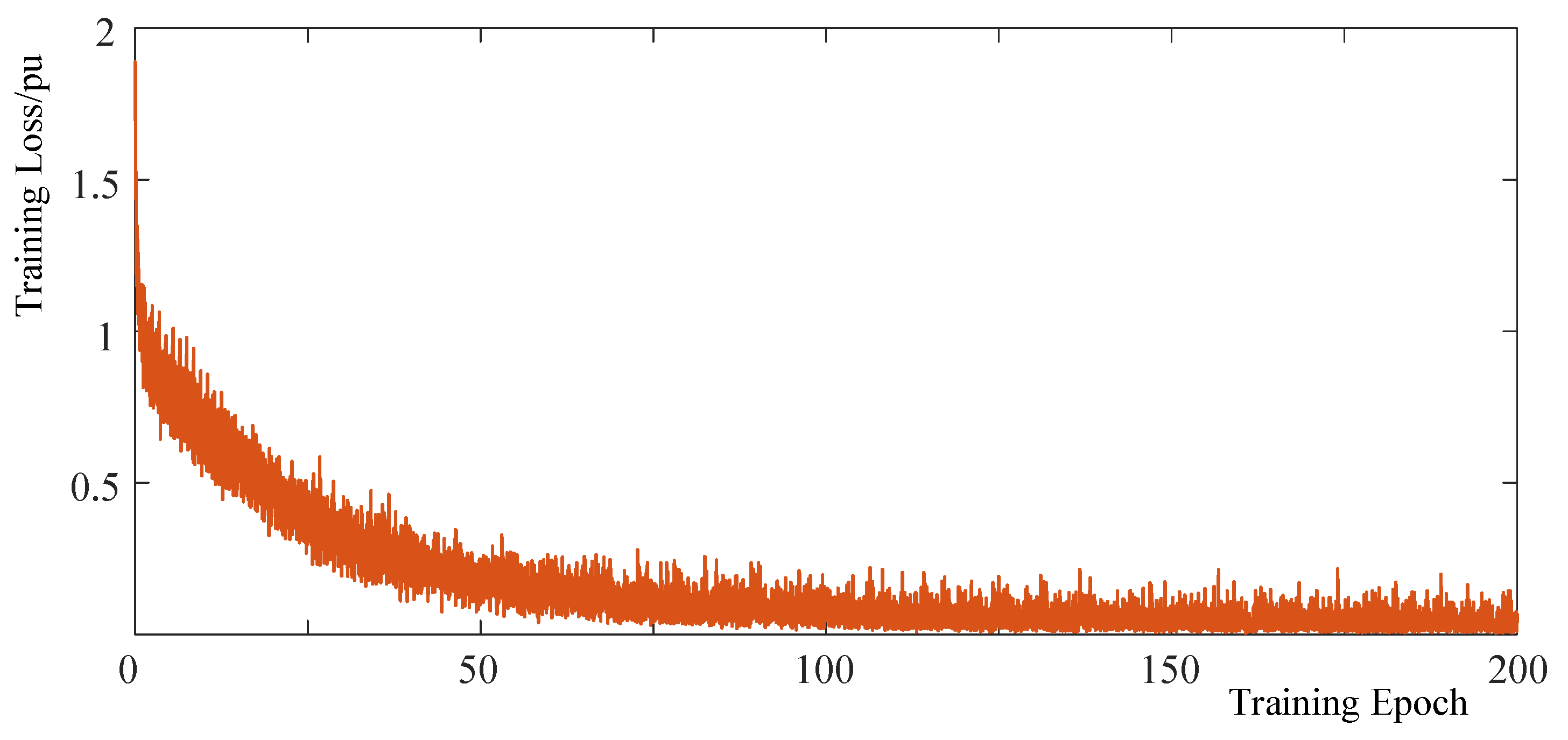
Further, the fine-tuning procedure of the TL framework was discussed with the illustration of the learning procedure. As shown in Figure 9, with the 300-case dataset fed into the TSA model transferred from the IEEE 39-bus system, the fine-tuning procedure converges rapidly in 100 epochs. This implies that the proposed TL framework can be implemented in a highly efficient manner, saving a large amount of time during TSA model fine-tuning.

4.3. Comparative Test

To further demonstrate the advantage of the proposed TL framework in tackling the TSA issue, comparative tests were performed. Specifically, some conventional ML methods introduced into existing data-driven DSA studies, including decision tree (DT) [30], support vector machine (SVM) [17], multilayer perceptron (MLP)-based neural network [31], eXtreme Gradient Boosting (XGBoost) [32], CNN [7], and CNN + LSTM [10], were considered for comparison. All of these comparative methods were provided with the same 9000-case training dataset generated in the GDPG for TSA model training, and the obtained models were fed with the same 3000-case testing dataset for performance evaluation. The corresponding test results are summarized in

Table 2. TSA Performance Comparisons (with 3000 Testing Cases Generated in GDPG).

Method	$\mathit{Mis}$/%	$\mathit{Fal}$/%	$\mathit{Acc}$/%
Proposed	0.80	0.37	98.83
DT	1.70	1.97	96.33
SVM	1.83	1.63	96.54
MLP	1.90	2.27	95.83
XGBoost	2.07	1.17	96.76
CNN	0.70	0.43	98.87
CNN + LSTM	0.43	0.67	99.90

.

As can be observed, the conventional DT, SVM, MLP, and XGBoost methods involving shallow learning structures fall behind the proposed TL framework, with much higher misdetection and false-alarm rates. On the contrary, the other two DL methods, i.e., CNN and CNN + LSTM, exhibit superior performances, with the overall TSA accuracy being a bit higher than that of the TL framework. However, it should be mentioned that the desirable performances of these DL methods are achieved at the cost of learning from a bulky training dataset with 9000 cases. As will be shown in subsequent tests, the preparation of such a large-size dataset would be extremely time-consuming (costing more than 1.5 days), making the whole offline learning procedure computationally prohibitive. In contrast, the proposed TL framework only requires the preparation of a small dataset with 300 cases, which would save large amounts of computation time during offline learning. Therefore, compared with the existing ML methods, the proposed method is able to achieve competitive DSA performances without introducing high computational costs into offline learning data preparation, being more applicable in practical large-scale power grids.

4.4. Computational Efficiency

With special attention to the TL-based TSA scheme borrowing stability knowledge from the IEEE 39-bus system and the conventional TSA solution directly learning from 9000 cases, their computation times in learning/testing procedures were recorded. As summarized in

Table 3. Summary of Computation Times (with/without TL).

Scheme	Offline Dataset Preparation/s	Offline TSA Model Training/s	Online Computation/s
With TL	18,174.234	1563.586	0.003
Without TL	163,684.732	2479.351	0.003

Note 2: The second column represents the total time consumption of offline transient case generation and data preprocessing; the third column stands for the time consumption of all the offline ML/DL procedures; the fourth column corresponds to the average computation times for the 3000 unseen cases during online TSA application.

, while both of them can rapidly carry out online TSA in less than 5 ms, the TL-based scheme has much lighter offline computational burdens than the latter. Specifically, with the help of TL, the total time consumption of offline dataset preparation is cut down by more than 40 h. This is mainly due to the fact that the number of learning cases for GDPG is largely reduced after the introduction of TL, which dramatically alleviates the computational burdens caused by batch TD simulations in the large-scale GDPG. Although thousands of cases also need to be prepared for the IEEE 39-bus system, with a much smaller size, its TD simulation efficiency is much higher than that of GDPG. Given the significant improvement of offline computational efficiency, the TL-based TSA scheme would be more helpful in practical contexts, where timely TSA model retraining/updating is required during online monitoring.

5. Conclusions

Aiming at transferring stability knowledge learned from test systems to practical power grids, this work proposes a light-weight TL framework for online DSA. Based on sale-free system feature learning and system dissimilarity quantification, it is able to strategically select appropriate test systems that generalize well to online DSA contexts in practice. As demonstrated in the realistic GDPG, this framework can significantly alleviate the offline computational burden of data-driven DSA without sacrificing its reliability. In future studies, more systematic learning schemes such as ensemble learning can be designed to leverage a set of similar test systems to further boost the DSA performances.