ELM-Based Adaptive Practical Fixed-Time Voltage Regulation in Wireless Power Transfer System

Abstract

This paper proposes an extreme learning machine (ELM)-based adaptive sliding mode control strategy for the receiver-side buck converter system in the wireless power transfer system subjecting to the lumped uncertainty. The proposed control strategy utilizes a singularity-free fixed-time sliding mode (FTSM) feedback control, which ensures a fixed-time convergence for both the sliding variable and voltage tracking error. An ELM-based uncertainty bound estimator is further designed to learn the uncertainty bound information in real-time, which opportunely loosens the constraint of bound information requirement for sliding mode control design. The global stability of the closed-loop system is rigidly analyzed, and the good performance of the proposed control strategy is validated by comparison experiments which exhibit ideal overshoot elimination, 45.70–51.72% reduction of settling time, and 13.65–36.96% reduction of the root mean square value for voltage tracking error with respect to different load types.

1. Introduction

Wireless power transfer (WPT) systems based on magnetic resonant coupling have been widely investigated in recent years [1]. Due to the merits of superior safety, convenience, reliability, efficiency, and medium transfer distance, the WPT can readily deliver power for various applications such as flexible wireless heating [2], dimmable wireless lighting [3], wireless charging for electric vehicles (EVs) [4,5], and wireless power and drive transfer (WPDT) system for electric motors [6,7,8]. Alongside serious successful applications for WPT, transmission efficiency varies significantly with changes in mutual inductance, phase shift angle, and load. For dealing with the phase shift variations in WPT system, literature [9] has proposed a discrete proportional-integral (PI) based switched-mode converter for series–series (SS) compensated WPT system, which features the elimination of direct communication between the transmitter side and the receiver side. However, the performance cannot be guaranteed with fast-dynamic variation in operation conditions, for instance, the load changes. For addressing the issues of dynamic response, the authors in [10] adopted a discrete sliding mode control (SMC) with PID-type sliding surface for SS compensated WPT system, which achieves significant small overshoot and settling time in comparison with PI control. However, the linear structure of sliding surface hinders the convergence property of the WPT system. Besides, the authors in [11] further investigated deep deterministic policy gradient (DDPG) based on an ultra-local model (ULM) control scheme for SS compensated WPT system, which validates an improvement of transient performance compared with SMC.

DC-DC converters, as a typical power regulator, have been widely employed in various WPT systems for flexibly adjusting the power of both transmitter and receiver sides. Nevertheless, precise and robust control for DC-DC converters remains challenging since DC-DC converters are highly susceptible to different kinds of disturbance and uncertainties introduced by parametric drifts, load variations, and input oscillations. In the literature, a variety of control methods are utilized to stabilize the DC-DC converters for the purpose of obtaining a high performance of power regulations, for instance, traditional linear control methods [12], model predictive control [13], optimal control [14,15,16], fuzzy logical control [17], etc. Although an acceptable stabilization performance can be obtained with the aforementioned control methods, the robustness and the convergence property of the closed-loop buck converter systems could be further improved, especially in sceneries of WPT systems, which are affected by multiple uncertainties, including coils distance, circuit operating condition changes, and external electromagnetic interference.

Owing to the good features of disturbance insensitiveness and superior steady and transient performance, SMC has attracted significant attention in control community in both linear and nonlinear systems [18,19,20]. Several SMC schemes have been introduced to DC-DC converters [21,22,23]. In [21], a hysteresis-modulated SMC was proposed to improve the dynamic voltage-tracking performance for DC-DC converters. The authors in [22] further investigated pulse-width-modulation (PWM)-based SMC, which successfully tackled the issue of variation of switching frequency in [21]. The authors in [23] proposed a duty-ratio based sliding mode control for buck converter with constant power loads (PCLs), which is capable of stabilizing power systems in a large range of operating conditions. For achieving a fast convergence property, terminal sliding mode (TSM) control has been further implemented for buck converters in [24,25,26,27]. With the introduction of a nonlinear sliding manifold, a finite time convergence for voltage regulation can be well guaranteed. Despite the fast dynamics response of TSM controls, one problem still impedes its theoretical development, namely, the convergence time will grow unboundedly if the initial value of the state approaches infinity. Within this context, literature [28,29,30] investigated fixed time stability theory, which ensures an upper-bounded convergence time that is independent of the initial value of the closed-loop system states.

Recently, the neural network (NN)-aided control method has drawn renewed attention due to its universal approximation capability [31,32,33,34,35,36,37,38]. In [33], the authors proposed an adaptive fuzzy-neural-network control (AFNNC) scheme to estimate a TSM control law for voltage tracking control of a boost converter. In [35], the authors addressed the destabilization effect of the CPLs under the reference voltage variations through a ULM control scheme with parameters being tuned by the deep reinforcement learning (DRL) technique. The authors in [36] utilized an artificial neural network to implement optimal control for buck converter based on approximate dynamic programming (ADP). In [37], a dynamic sliding mode control was designed for boost converter where the uncertainty of the system is learned by a type-2 fuzzy neural network. In [38], the authors proposed a deep learning approach which uses offline experimental data to model the behavior of buck converters. One drawback of NN-aided control is that the input and output weights of the NNs are tunned simultaneously by utilizing gradient descent algorithms, which significantly hinders the application of real-time closed-loop systems due to their low learning rate and high sensitivity toward the training data. To tackle this problem, a novel neural network, namely, extreme learning machine (ELM), has been proposed in [39], which features an extremely fast learning rate and significant generalization property since only output weights need to be trained, and its excellent performance in the closed-loop system has been verified in the literature [40,41,42,43].

Inspired by the fixed time control theory and ELM technique, this paper revisits the voltage tracking issue of receiver-side buck converters in WPT systems. The uncertainty model of the WPT-buck system is first established with the consideration of perturbation of the input inductor, output capacitor, load variations, and external disturbance.

Secondly, a fixed time sliding mode (FTSM) control was proposed with an ELM estimator for learning the upper-bound of the lumped disturbance. The main feature of ELM-aided control in this paper is that the adopted ELM mechanism is integrated into the closed-loop control system, which eliminates the conventional weights training process. Accordingly, despite the same structure and input weights assignment approaches shared with conventional ELM for pattern classifications, the output weights of the adaptive ELM mechanism utilized in this paper are updated based on Lyapunov second theory, which aims to ensure global stability of the closed-loop system. The main contributions of this paper are listed as follows:

(1)

A fixed time voltage regulation of the closed-loop WPT-buck system is guaranteed without singularity, which, to the best of our knowledge, is the first time to study the voltage regulation issue for WPT-buck system in a fixed time horizon.

(2)

For the adopted ELM, not only is the training process eliminated, but the lumped uncertainty bound is learned in real-time via an ELM structure with only output measurements, which ideally alleviates the requirement of disturbance information in traditional SMC designs.

(3)

The fixed time convergence of system states, sliding variable, and output weights of ELM has been rigorously proved based on Lyapunov second theory.

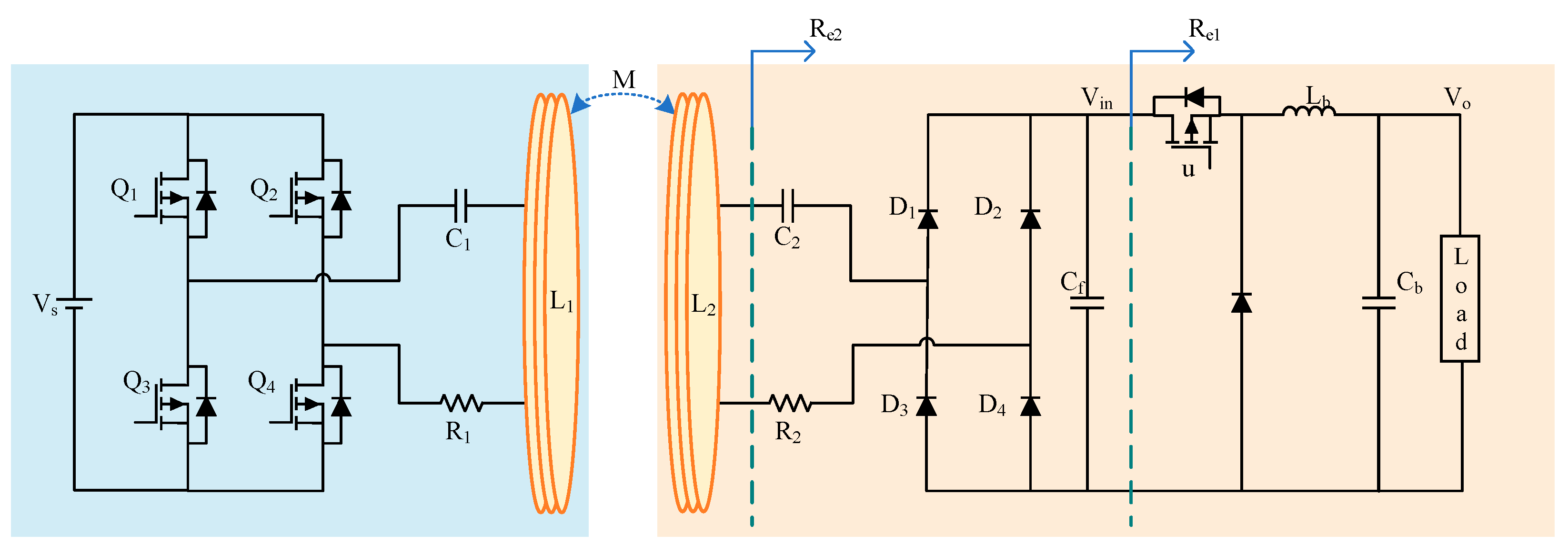
The rest of the paper is organized in the following manner. In Section 2, the model of WPT-buck system is formulated with unknown dynamics, parameters variation, and unknown disturbance. An introduction of SLFN with ELM algorithm is given in Section 3. The proposed fixed time sliding mode control with ELM disturbance upper-bound estimator is designed in Section 4. The experimental study is conducted in Section 5 as compared with PI control schemes. Finally, the conclusion of the paper is drawn in Section 6.

2. Plant Modelling

Figure 1 shows the basic diagram of a series–series (SS) compensated WPT system. A typical WPT system includes a high-frequency AC source, magnetic coupling component which is comprised of a power transmitter coil and power receiver coil, power regulation circuit, and terminal load. The basic workflow of WPT system is as follows. The high-frequency power source is first obtained through a full-bridge inverter. Power is then transferred from the transmitter coil to the receiver coil through two resonance circuits. After a rectifier circuit, the terminal load catches power through proper regulation, for instance, Buck, Boost, or Cuk circuits.

A typical full-bridge invertor consists of four switches and is controlled via pulse width modulation (PWM) module. The output voltage of full-bridge invertor can be obtained by first-order harmonic approximation as follows:

$$V_1=\frac{4V_s}{\pi }\sin \left({\omega }_{0}t\right)$$

(1)

where $V_s$ is the DC power supply voltage, ${\omega }_0={\left[1/\left(L_1{C}_1\right)\right]}^{1/2}={\left[1/\left(L_2{C}_2\right)\right]}^{1/2}=2\pi f_0$ is the resonant angular frequency of the WPT system.

The relationship between input and output resistance for rectifier circuit and buck converter operates at CCM can be obtained as [44]

$$R_{e2}=\frac{8}{{\pi }^2}{R}_{e1}$$

(2)

$$R_{e1}=\frac{1}{D^2}{R}_L$$

(3)

where $D\in \left(0,1\right)$ is the duty cycle of the buck converter and $R_L$ denotes the equivalent load resistance.

Recalling the T-type equivalent circuit mode of Figure 1 with equivalent resistance given in (2) and (3), and using the Kirchhoff’s Voltage Law, the linearized circuit model can be formulated as:

$$\begin{array}{c}{V}_1=\left[R_1+j\left({\omega }_0{L}_1-\frac{1}{{\omega }_0{C}_1}\right)\right]I_1-j{\omega }_{0}M{I}_2\\ 0=\left[R_{e2}+R_2+j\left({\omega }_0{L}_2-\frac{1}{{\omega }_0{C}_2}\right)\right]I_2-j{\omega }_{0}M{I}_1\end{array}$$

(4)

where $C_1$ and $C_2$ represent the primary and secondary capacitors. $I_1$ and $I_2$ are the current through the transmitter coil equivalent inductor $L_1$ and the receiver coil equivalent inductor $L_2$. $M$ represents the mutual inductor through two coils. $R_1$ and $R_2$ are equivalent resistances on two sides which are comprised of inductor resistance, capacitor series resistance, and switch resistance of the bridge. The secondary current $I_2$ can be obtained as:

$$I_2=\frac{-j{\omega }_{0}M{V}_1}{\left(R_1+X_1\right)\left(R_2+R_{e2}+X_2\right)+{\omega }_0^2{M}^2}$$

(5)

where $X_1=j\left[{\omega }_0{L}_1-1/\left({\omega }_0{C}_1\right)\right]$ and $X_2=j\left[{\omega }_0{L}_2-1/\left({\omega }_0{C}_2\right)\right]$. Given that the system is operated under the resonant frequency, the secondary current and output voltage can be derived as:

$$I_2=\frac{-j{\omega }_{0}M{V}_1}{R_1\left(R_2+R_{e2}\right)+{\omega }_0^2{M}^2}=A\sin \left({\omega }_{0}t-\frac{\pi }{2}\right)$$

(6)

$$V_2=I_2{R}_{e2}=V_{in}\sin \left({\omega }_{0}t-\frac{\pi }{2}\right)$$

(7)

where $V_{in}=8A/\left(\pi D^2\right)$, $A=4V_s{\omega }_{0}M/\left[\pi R_1\left(R_2+R_{e2}\right)+\pi {\omega }_0^2{M}^2\right]$.

In this paper, a buck converter is applied as power regulation, and the average model of the converter in the continuous conduction mode (CCM) can be formulated as follows:

$$\begin{array}{c}{L}_b\frac{d{I}_L}{dt}=V_{in}D-V_o\\ C_b\frac{d{V}_o}{dt}=I_L-\frac{V_o}{R}-I_{dis}\end{array}$$

(8)

where $L_b$ and $C_b$ are inductor and conductor of buck converter, $V_o$ is the output voltage drops on load, $I_L$ is the current in inductor $L_b$, and $I_{dis}$ is the disturbance current. Denoting the desired output voltage as $V_d$, the tracking error can be obtained as $x_1=V_o-V_d$. Following that, selecting $x_2={\dot{x}}_1=\frac{I_L}{C_b}-\frac{V_o}{R{C}_b}$, a state space model can be obtained as:

$$\begin{array}{c}{\dot{x}}_1=x_2\\ {\dot{x}}_2=\frac{V_{in}}{C_b{L}_b}D-\frac{V_o}{C_b{L}_b}-\frac{1}{R{C}_b^2}\left(I_L-\frac{V_o}{R}\right)-\frac{I_{dis}}{R{C}_b^2}\end{array}$$

(9)

It is noted that in real scenarios, the values of circuit parameters vary in real time due to wearing and aging. In this work, such uncertainties are modelled as follows:

$$C_b=C_{b0}+\mathsf{\Delta }{C}_b$$

(10)

$$L_b=L_{b0}+\mathsf{\Delta }{L}_b$$

(11)

$$V_{in}=V_{in0}+\mathsf{\Delta }{V}_{in}$$

(12)

$$R=R_0+\mathsf{\Delta }R$$

(13)

where $C_{b0}$, $L_{b0}$, $V_{in0}$, and $R_0$. are nominal terms with their corresponding values given in

Table 1. Nominal parameter values of WPT-buck system.

Parameters	Values
$C_{b0}$, $C_1$, $C_2$, $C_f$	$5\times {10}^5$, 42.7, 42.7, $3.4\times {10}^5$ (nF)
$L_{b0}$, $L_1$, $L_2$, $M$	100, 82, 82, 16 ($\mathsf{\mu }\mathrm{H}$)
$R_1$, $R_2$, $R_0$	0.135, 0.133, 10 ($\mathsf{\Omega }$)
$V_{in0}$	32 (V)
$f_b$, $f_0$	20, 85 ($\mathrm{kHz}$)

, and $\mathsf{\Delta }{C}_b$, $\mathsf{\Delta }{L}_b$, $\mathsf{\Delta }{V}_{in}$, and $\mathsf{\Delta }R$ represent the parameter uncertainties. Redefining $x_2=\frac{I_L}{C_{b0}}-\frac{V_o}{R_0{C}_{b0}}$, an uncertainty model of buck converter can then be further reformulated as:

$$\begin{array}{c}{\dot{x}}_1=x_2+d_1\\ {\dot{x}}_2=u-\frac{V_o}{C_{b0}{L}_{b0}}-\frac{1}{R_0{C}_{b0}^2}\left(I_L-\frac{V_o}{R_0}\right)+d_2\end{array}$$

(14)

where $u=D{V}_{in0}/\left(C_{b0}{L}_{b0}\right)$, $d_1=\left(1/C_b-1/C_{b0}\right)I_L+\left[1/\left(R_0{C}_{b0}\right)-1/\left(R{C}_b\right)\right]V_o$, $d_2=\left[\left(D{V}_{in0}-V_o\right)L_b{C}_b-\left(D{V}_{in}-V_o\right)L_{b0}{C}_{b0}\right]/\left(L_b{C}_b{L}_{b0}{C}_{b0}\right)+\left(R{C}_b{x}_2-R_0{C}_{b0}{x}_2-R_0{C}_{b0}{d}_1\right)/\left(R_0{C}_{b0}R{C}_b\right)-I_{dis}/R{C}_b^2$. Note that the systems’ uncertainties can be regarded as disturbances from the viewpoint of system synthesis. It can be thus observed from (14) that there are both matched and mismatched disturbances in voltage error dynamic system. By the definitions of the disturbances $d_1$ and $d_2$, one knows that they are generally bounded in practice, i.e., there are some known constants ${\overline{d}}_1$ and ${\overline{d}}_2$ to make the following conditions hold: $\left|d_1\right|\le {\overline{d}}_1$ and $\left|d_2\right|\le {\overline{d}}_2$.

3. Brief Review of ELM

ELM, first unveiled in the work of [39], adopts the same structure of SLFN with an input layer, a hidden layer, and output layer that are distinguished from the traditional weights training process based on gradient-descent in most SLFN, like BP algorithms. ELM randomly determines the input weights between the input layer and hidden layer and maintains its value unchanged. Thus, only the output weighs training process is required, which significantly fastens the parameter updating of the SLFN. Such characteristics have proved to be an efficient method in real-world applications.

Assuming there is a distinct training set $\varnothing =\left\{\left(x_i,t_i\right)|x_i\in R^n,t_i\in R^m,i=1,\dots ,N\right\}$, an ELM with $L$ hidden nodes can be defined as:

$$\stackrel{L}{\sum _{i=1}}{\beta }_{i}g\left(x_j,{\omega }_i, z_i\right)=t_j,\hspace{1em}j=1,\cdots ,N$$

(15)

where ${\omega }_i\in R^n$ is the input weight vector connecting input layer and hidden layer, $z_i$ is the input bias of the hidden layer, ${\beta }_i\in R^m$ is the output weight vector, and $g(\cdot )$ is the activation function. ELM can approximate the data samples with zero error with enough noes in a hidden layer:

$$H\left(x,\omega ,z\right)\beta =T$$

(16)

where $H\left(x,\omega ,z\right)={\left[\begin{array}{ccc}g\left(x_1,{\omega }_1,z_1\right)& \cdots & g\left(x_1,{\omega }_L,z_L\right)\\ ⋮& \cdots & ⋮\\ g\left(x_N,{\omega }_1,z_1\right)& \cdots & g\left(x_N,{\omega }_L,z_L\right)\end{array}\right]}_{N\times L}$ is the so-called hidden layer output matrix of ELM [39], $x=\left[x_1,x_2,\cdots ,x_N\right]$, $\omega =\left[{\omega }_1,{\omega }_2,\cdots ,{\omega }_L\right]$, $z=\left[z_1,z_2,\cdots ,z_L\right]$, $\beta ={\left[{\beta }_1^T,\dots ,{\beta }_L^T\right]}^T\in R^{L\times m}$ and $T={\left[t_1^T,t_2^T,\cdots ,t_N^T\right]}^T\in R^{N\times m}$.

Since the input weight $\omega$ and the hidden layer biases $z$ are determined in advance, the training process of ELM can be thus simplified to finding the solution of linear system $H\left(x,\omega ,z\right)\beta =T$ as

$$\Vert H\left(x,\omega ,z\right)\widehat{\beta }-T\Vert =\underset{\beta }{\min }\Vert H\left(x,\omega ,z\right)\beta -T\Vert$$

(17)

The unique smallest norm least-squares solution of (17) is:

$$\widehat{\beta }=H^{†}\left(x,\omega ,z\right)T$$

(18)

where $H^{†}\left(x,\omega ,z\right)$ indicates the Moore–Penrose generalized inverse form of matrix $H\left(x,\omega ,z\right)$. Provided that the activation function is infinitely differentiable in any interval, there always exists a theorem for $N$ arbitrary distinct samples $\left(x_i,t_i\right)\in R^{n\times m}$ with random $\omega$ and $\alpha$ generated from any interval of $R^n$ and $R$, with probability one,

$$\Vert H\left(x,\omega ,z\right)\beta -T\Vert =\Vert \epsilon \left(x\right)\Vert <{\epsilon }_1$$

(19)

where $\epsilon \left(x\right)$ is approximation error and ${\epsilon }_1$ is a known positive value.

4. Controller Design

To achieve a robust fixed time convergence without singularity, a nonsingular fixed sliding mode control scheme is designed, and the uncertainty bound is learned online via ELM estimator.

4.1. Notations and Lemmas

Throughout the paper, the following notations will be used: (1) For any non-negative real number $\alpha$, the function $x\mapsto {\lceil x\rfloor }^{\alpha }$ is defined as ${\lceil x\rfloor }^{\alpha }={\left|x\right|}^{\alpha }\mathrm{sign}\left(x\right)$ for $x\in R$. It follows from the definition that $d{\lceil x\rfloor }^{\alpha }/dx=\alpha {\left|x\right|}^{\alpha -1}$, ${\lceil x\rfloor }^0=\mathrm{sign}\left(x\right)$, $\lceil x\rfloor =x$ and ${\lceil x\rfloor }^{\alpha }{\lceil x\rfloor }^{\beta }={\left|x\right|}^{\alpha +\beta }$. (2) For any $\beta ={\left[{\beta }_1,{\beta }_2,\cdots ,{\beta }_n\right]}^T\in R^n$, we define ${\beta }^{\alpha }={\left[{\beta }_1^{\alpha },{\beta }_2^{\alpha },\cdots ,{\beta }_n^{\alpha }\right]}^T$. Besides, some lemmas and standard definitions are given here that are utilized in the paper.

Definition 1

[45]. The origin of the system (14) is globally fixed-time stable if it is globally finite-time stable and the settling time function $T$ is bounded, i.e., $\exists T>0: T\le T_{max}, \forall x_0\in R^n$. Therefore, the settling time is always bonded regardless of system initial conditions in fixed-time control methods.

Lemma 1

[45]. Consider $r_1,r_2,\cdots ,r_n\in R_{+}$ and $0<\gamma <2$, then we have:

$$\stackrel{n}{\sum _{i=1}}{r}_i^{\gamma }\ge {\left(\stackrel{n}{\sum _{i=1}}{r}_i^2\right)}^{\frac{\gamma }{2}}$$

(20)

Lemma 2

[45]. Consider $r_1,r_2,\cdots ,r_n\in R_{+}$ and $0<b\le 1$ and $c>1$, then we have:

$$\stackrel{n}{\sum _{i=1}}{r}_i^b\ge {\left(\stackrel{n}{\sum _{i=1}}{r}_i\right)}^b, \stackrel{n}{\sum _{i=1}}{r}_i^j\ge n^{1-j}{\left(\stackrel{n}{\sum _{i=1}}{r}_i\right)}^j$$

(21)

Lemma 3

[45]. For any ${\kappa }_1,{\kappa }_2>0$ , $0<{\varpi }_1<1<{\varpi }_2$ , $0<\Gamma <\infty$, and a continuously differentiable positive function $V\left(x\right):R^n\to R_{+}$ such that $V\left(x\right)=0$ for $x\left(t\right)=0$. If any solution $x\left(t\right)$ of (14) satisfies the inequality $\dot{V}\left(x\right)\le -{\kappa }_1{V}^{{\varpi }_1}\left(x\right)-{\kappa }_2{V}^{{\varpi }_2}\left(x\right)+\Theta$, the system is fixed-time stable and the convergent region is bounded by

$$\mathsf{\Delta }=\left\{x|V\left(x\right)\le \min \left\{{\left(\frac{\mathsf{\Theta }}{\left(1-\theta \right){\kappa }_1}\right)}^{\frac{1}{{\varpi }_1}},{\left(\frac{\mathsf{\Theta }}{\left(1-\theta \right){\kappa }_2}\right)}^{\frac{1}{{\varpi }_2}}\right\}\right\}$$

(22)

where $0<\theta <1$ is a constant. The settling time is bounded by

$$T\le T_{max}=\frac{1}{{\kappa }_1\left(1-{\varpi }_1\right)}+\frac{1}{{\kappa }_2\left({\varpi }_2-1\right)}$$

(23)

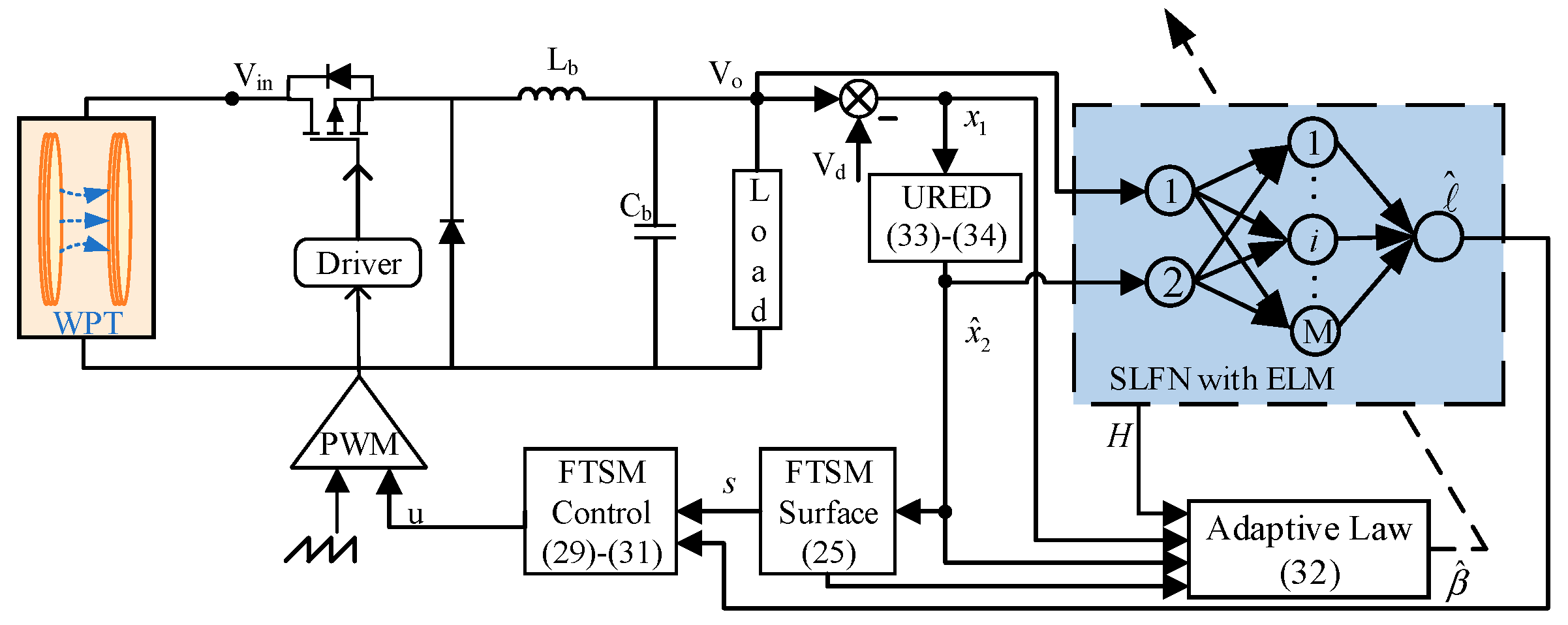
4.2. Controller Design

First, a nonsingular terminal sliding variable is given as:

$$s=\lceil x_1\rfloor {}^{{\alpha }_1}+c^{\prime }{\lceil \sigma \rfloor }^{{\alpha }^{\prime }}$$

(24)

$$\sigma =x_2+c_1\lceil x_1\rfloor {}^{{\alpha }_1}$$

(25)

where $1<{\alpha }_1<{\alpha }^{\prime }$, ${\alpha }^{\prime }=2-1/{\alpha }_2$ with ${\alpha }_2>1$, $c^{\prime }=c_2/{\alpha }^{\prime }$, $c_1$, $c_2$ are all positive constants.

Then, the unknown upper-bound of the matched disturbance, denoted by $\ell$, is modeled as the output of an SLFN, which is formulated in the form of:

$$\ell =H\left(y,\omega ,z\right){\beta }^{*}+{\epsilon }_n\left(y\right)$$

(26)

where $H\left(y,\omega ,z\right)=\left[g\left(y,{\omega }_1,z_1\right),\cdots ,g\left(y,{\omega }_{\tilde{M}},z_{\tilde{M}}\right)\right]$ is the so-called hidden layer matrix [39] and $\tilde{M}$ denotes the number of hidden layer nodes of the proposed ELM, $y={\left[V_o,{\dot{V}}_o\right]}^T$ presents the input vector. ${\beta }^{*}={\left[{\beta }_1^{*},\cdots ,{\beta }_{\tilde{M}}^{*}\right]}^T$ is the optimal output weight vector of ELM. ${\epsilon }_n\left(y\right)$ is the approximating error. According to ELM universal approximation theory [39], we can validate the assumption that the estimation ${\epsilon }_n\left(y\right)$ is upper-bounded with an arbitrary positive constant, i.e., $\left|{\epsilon }_n\left(y\right)\right|\le {\epsilon }_N$. For the real application, the optimal value ${\beta }^{*}$ is not available, thus we define the estimated value of $\ell$ as follows:

$$\widehat{\ell }=H\widehat{\beta }$$

(27)

where $\widehat{\beta }$ is the estimation of ${\beta }^{*}$, and $H$ is the abbreviation of $H\left(y,\omega ,z\right)$.

The proposed control law is then designed as below:

$$u=u_0+u_1$$

(28)

$$u_0=-f_0-c_1{\alpha }_1{\left|x_1\right|}^{{\alpha }_1-1}{x}_2-c_1{\left|x_1\right|}^{{\alpha }_1-1}\left(\frac{{\lceil \sigma \rfloor }^{2-{\alpha }^{\prime }}}{c_2}+c^{\prime }\sigma \right)$$

(29)

$$u_1=-\left(\widehat{\ell }+{\rho }_0\right){\lceil s\rfloor }^0-{\rho }_{1}s-{\rho }_2{\lceil s\rfloor }^{\mu }$$

(30)

where $f_0=-\frac{V_o}{C_{b0}{L}_{b0}}-\frac{1}{R_0{C}_{b0}^2}\left(I_L-\frac{V_o}{R_0}\right)$, ${\rho }_0$ is chosen to be sufficiently large such that ${\rho }_0>{\epsilon }_N$ and ${\rho }_1,{\rho }_2>0$, $\mu >1$ are the parameters to be determined. Furthermore, the estimated output weight $\widehat{\beta }$ of ELM estimator for constructing $\widehat{\ell }$ is updated online by the following adaptive law:

$${\dot{\widehat{\beta }}}^T={\eta }_1\varphi \left(H\left|s\right|-{\iota }_1{\widehat{\beta }}^T\right)$$

(31)

where ${\eta }_1, {\iota }_1$ are designed positive constants, $\varphi =c_2{\left|\sigma \right|}^{{\alpha }^{\prime }-1}$.

To address the issue of large measuring noise in inductance current, we adopted a uniform robust exact differentiator (URED) [46] to obtain the estimation for the state of $x_2$ in the form of:

$${\dot{\varsigma }}_0={\varsigma }_1-{\lambda }_1\left(\lceil {\tilde{x}}_1\rfloor {}^{1/2}+\xi \lceil {\tilde{x}}_1\rfloor {}^{3/2}\right)$$

(32)

$${\dot{\varsigma }}_1=-{\lambda }_2\left(\lceil {\tilde{x}}_1\rfloor {}^0/2+2\xi {\tilde{x}}_1+3{\xi }^2\lceil {\tilde{x}}_1\rfloor {}^2/2\right)$$

(33)

where ${\tilde{x}}_1={\widehat{x}}_1-x_1$, with ${\widehat{x}}_1$ being the estimation of $x_1$, ${\lambda }_1$, ${\lambda }_2$, and $\xi$ are positive parameters which are chosen as ${\lambda }_1=1$, ${\lambda }_2=3$, $\xi =5$ in our study. It has been proven that if $\left|x_1\left(t\right)\right|\le \varrho$, with some positive constants ${\nu }_0$, ${\nu }_1$, one has the following inequality [46]

$$\left|{\varsigma }_0-x_1\right|<{\nu }_0\varrho$$

(34)

$$\left|{\varsigma }_1-x_2\right|<{\nu }_1{\varrho }^{1/2}$$

(35)

being established with convergence time upper-bounded by some constants.

The block diagram of the proposed voltage tracking control scheme with ELM estimator is shown in Figure 2. In the following subsection, the global closed-loop stability based on fixed time theory will be elaborated.

4.3. Stability Analysis

For the global closed-loop stability analysis, the following theorem is given firstly:

Theorem 1.

Consider the closed-loop buck system in (14) with parametric variations given by (10)–(13). The output tracking error converges to a residual set of origin under the control law designed in (28) in a time$T$is bounded by:

$$T<T_f=T_s+T_e+\epsilon \left({\tau }_1\right)$$

(36)

where$T_s=1/\left[k_1\left(1-n_1\right)\right]+1/\left[k_2\left(n_2-1\right)\right]$with$k_1$,$k_2$,$n_1$,$n_2$being positive constants to be determined.$T_e=1/\left[c_1\left({\alpha }_1-1\right)\right]+1/\left[{\left({\alpha }^{\prime }/c_2\right)}^{1/{\alpha }^{\prime }}\left(1-{\alpha }_1/{\alpha }^{\prime }\right)\right]$and$\epsilon \left({\tau }_1\right)$represents a small time margin related to the boundary width${\tau }_1={\left(1/c_2\right)}^{{\alpha }^{\prime }-1}$.

Proof. 

First, substituting the control law (28) into (24), the dynamic of sliding variable can be given as:

$$\dot{s}={\alpha }_1{\left|x_1\right|}^{{\alpha }_1-1}{x}_2+\varphi \left({\dot{x}}_2+c_1\lceil x_1\rfloor {}^{{\alpha }_1}+c_1{\alpha }_1{\left|x_1\right|}^{{\alpha }_1-1}{x}_2\right)$$

(37)

With the definition given by (24), we have the following relationship:

$$\varphi \left(\frac{1}{c_2}{\lceil \sigma \rfloor }^{2-{\alpha }^{\prime }}+\frac{c_1}{{\alpha }^{\prime }}\sigma \right)=x_2+c_{1}s$$

(38)

Substituting (38) into (37), one has:

$$\dot{s}=-{\alpha }_1{c}_1{\left|x_1\right|}^{{\alpha }_1-1}s-\varphi \left[\left(\widehat{\ell }+{\rho }_0\right){\lceil s\rfloor }^0+{\rho }_{1}s+{\rho }_2{\lceil s\rfloor }^{\mu }-d_2\right]$$

(39)

Then, a Lyapunov candidate can be chosen as follows:

$$V=0.5s^2+0.5{\eta }_1^{-1}{\tilde{\beta }}^T\tilde{\beta }$$

(40)

where $\tilde{\beta }={\beta }^{*}-\widehat{\beta }$. Taking the first derivative of $V$, we have:

$$\begin{array}{c}\dot{V}=s\dot{s}+{\eta }_1^{-1}{\tilde{\beta }}^T\tilde{\beta }\\ \hspace{1em}=-\varphi \left(\widehat{\ell }+{\rho }_0\right)\left|s\right|-\varphi d_{2}s-\varphi {\rho }_1{s}^2-\varphi {\rho }_2{\left|s\right|}^{\mu +1}+{\eta }_1^{-1}{\dot{\tilde{\beta }}}^T\tilde{\beta }\\ \hspace{1em}=-\varphi \left(\widehat{\ell }-\ell +{\rho }_0\right)\left|s\right|-\varphi {\rho }_1{s}^2-\varphi {\rho }_2{\left|s\right|}^{\mu +1}-\varphi \left(H\left|s\right|-{\iota }_1{\widehat{\beta }}^T\right)\tilde{\beta }\\ \hspace{1em}=-\varphi \left(H\tilde{\beta }+{\epsilon }_n\left(z\right)+{\rho }_0\right)\left|s\right|-\varphi {\rho }_1{s}^2-\varphi {\rho }_2{\left|s\right|}^{\mu +1}-\varphi \left(H\left|s\right|-{\iota }_1{\widehat{\beta }}^T\right)\tilde{\beta }\\ \hspace{1em}\le -\varphi \left({\rho }_0-{\epsilon }_N\right)\left|s\right|-\varphi {\rho }_1{s}^2-\varphi {\rho }_2{\left|s\right|}^{\mu +1}+\varphi {\iota }_1{\widehat{\beta }}^T\tilde{\beta }\end{array}$$

(41)

Note that for any scalar ${\vartheta }_1>0.5$, we have:

$$\begin{array}{c}\varphi {\iota }_1{\widehat{\beta }}^T\tilde{\beta }=\varphi {\iota }_1\left(-{\tilde{\beta }}^T+{\beta }^{*}{}^T\right)\tilde{\beta }\\ \hspace{1em}\hspace{1em}\hspace{1em}\le -\varphi \frac{{\iota }_1\left(2{\vartheta }_1-1\right)}{2{\vartheta }_1}{\tilde{\beta }}^T\tilde{\beta }+\varphi \frac{{\iota }_1{\vartheta }_1}{2}{\beta }^{*}{}^T{\beta }^{*}\end{array}$$

(42)

Substituting (42) into (41) yields:

$$\begin{array}{c}\dot{V}\le -\varphi {\rho }_1{s}^2-\varphi \frac{{\iota }_1\left(2{\vartheta }_1-1\right)}{2{\vartheta }_1}{\tilde{\beta }}^T\tilde{\beta }+\varphi \frac{{\iota }_1{\vartheta }_1}{2}{\beta }^{*}{}^T{\beta }^{*}\\ \hspace{1em}\le -\phi V+\gamma \end{array}$$

(43)

where $\phi =\min \left\{2\varphi {\rho }_1,\varphi {\eta }_1\frac{{\iota }_1\left(2{\vartheta }_1-1\right)}{{\vartheta }_1}\right\}$, $\gamma =\varphi \frac{{\iota }_1{\vartheta }_1}{2}{\beta }^{*}{}^T{\beta }^{*}$, which means that the variables $s$ and $\tilde{\beta }$ are ultimately upper-bounded (UUB). Thus, there is a constant ${ϵ}_1$ such that $\Vert \tilde{\beta }\Vert <{ϵ}_1$ is always ensured.

Then, recalling (41), one has:

$$\dot{V}\le -\varphi {\rho }_3\left|s\right|-\varphi {\rho }_2{\left|s\right|}^{\mu +1}-\varphi {\left(\frac{{\chi }_1}{2{\eta }_1}{\Vert \tilde{\beta }\Vert }^2\right)}^{\frac{1}{2}}-\varphi {\left(\frac{{\chi }_1}{2{\eta }_1}{\Vert \tilde{\beta }\Vert }^2\right)}^{\frac{\mu +1}{2}}+{\theta }_1$$

(44)

where ${\theta }_1=-\varphi \frac{{\chi }_1}{{\eta }_1}{\tilde{\beta }}^T\tilde{\beta }+\varphi \frac{{\iota }_1{\vartheta }_1}{2}{\beta }^{*}{}^T{\beta }^{*}+\varphi {\left[\frac{{\chi }_1}{2{\eta }_1}\Vert \tilde{\beta }\Vert \right]}^{\frac{1}{2}}+\varphi {\left[\frac{{\chi }_1}{2{\eta }_1}\Vert \tilde{\beta }\Vert \right]}^{\frac{\mu +1}{2}}$, ${\chi }_1={\eta }_1\frac{{\iota }_1\left(2{\vartheta }_1-1\right)}{2{\vartheta }_1}$, ${\rho }_3={\rho }_0-{\epsilon }_N$.

If $\frac{{\chi }_1}{2{\eta }_1}{\Vert \tilde{\beta }\Vert }^2\ge 1$, it yields:

$$\varphi {\left(\frac{{\chi }_1}{2{\eta }_1}{\Vert \tilde{\beta }\Vert }^2\right)}^{\frac{1}{2}}+\varphi {\left(\frac{{\chi }_1}{2{\eta }_1}{\Vert \tilde{\beta }\Vert }^2\right)}^{\frac{\mu +1}{2}}-\varphi \frac{{\chi }_1}{{\eta }_1}{\Vert \tilde{\beta }\Vert }^2\le \varphi \left[{\left(\frac{{\chi }_1}{2{\eta }_1}{\Vert \tilde{\beta }\Vert }^2\right)}^{\frac{\mu +1}{2}}-\left(\frac{{\chi }_1}{2{\eta }_1}{\Vert \tilde{\beta }\Vert }^2\right)\right]$$

(45)

Otherwise, if $\frac{{\chi }_1}{2{\eta }_1}{\Vert \tilde{\beta }\Vert }^2<1$, it yields

$$\begin{array}{c}\varphi {\left(\frac{{\chi }_1}{2{\eta }_1}{\Vert \tilde{\beta }\Vert }^2\right)}^{\frac{1}{2}}+\varphi {\left(\frac{{\chi }_1}{2{\eta }_1}{\Vert \tilde{\beta }\Vert }^2\right)}^{\frac{\mu +1}{2}}-\varphi \frac{{\chi }_1}{{\eta }_1}{\Vert \tilde{\beta }\Vert }^2\le \varphi \left[{\left(\frac{{\chi }_1}{2{\eta }_1}{\Vert \tilde{\beta }\Vert }^2\right)}^{\frac{1}{2}}-\left(\frac{{\chi }_1}{2{\eta }_1}{\Vert \tilde{\beta }\Vert }^2\right)\right]\\ \hspace{1em}\hspace{1em}\hspace{1em}\hspace{1em}\hspace{1em}\hspace{1em}\hspace{1em}\hspace{1em}\hspace{1em}\hspace{1em}\hspace{1em}\hspace{1em}\hspace{1em}\hspace{1em}\hspace{1em}\hspace{1em}\hspace{0.17em}\hspace{0.17em}\le \varphi {\delta }_0\end{array}$$

(46)

where ${\delta }_0=r_0^{\frac{r_0}{1-r_0}}-r_0^{\frac{1}{1-r_0}}$ and $r_0=0.5$. Combining the results of (45) and (46) and recalling that $\Vert \tilde{\beta }\Vert \le {ϵ}_1$, the following inequality holds:

$$\begin{array}{c}{\left(\frac{{\chi }_1}{2{\eta }_1}{\Vert \tilde{\beta }\Vert }^2\right)}^{\frac{1}{2}}+\varphi {\left(\frac{{\chi }_1}{2{\eta }_1}{\Vert \tilde{\beta }\Vert }^2\right)}^{\frac{\mu +1}{2}}-\varphi \frac{{\chi }_1}{{\eta }_1}{\Vert \tilde{\beta }\Vert }^2\\ \le \varphi {\gamma }_1=\{\begin{array}{c}\varphi {\delta }_0\hspace{1em}\hspace{1em}\hspace{1em}\hspace{1em}\hspace{1em}\hspace{1em}\hspace{1em}\hspace{1em}\hspace{1em}{ϵ}_1\le \sqrt{\frac{2{\eta }_1}{{\chi }_1}}\\ \varphi \left[{\left(\frac{{\chi }_1{ϵ}_1^2}{2{\eta }_1}\right)}^{\frac{\mu +1}{2}}-\frac{{\chi }_1{ϵ}_1^2}{2{\eta }_1}\right] {ϵ}_1>\sqrt{\frac{2{\eta }_1}{{\chi }_1}}\end{array} \end{array}$$

(47)

Based on (47), (43) can be reformulated as:

$$\dot{V}\le -\varphi \left(k_1{V}^{n_1}+k_2{V}^{n_2}-{\gamma }_1\right)$$

(48)

where $n_1=\frac{1}{2}$, $n_2=\frac{\mu +1}{2}$, $k_1=\min \left\{{\rho }_3{2}^{n_1},{\chi }_1^{n_1}\right\}$, $k_2=\min \left\{{\rho }_2{2}^{n_2}{2}^{\frac{1-\mu }{2}},{\chi }_1^{n_2}{2}^{\frac{1-\mu }{2}}\right\}$. Note that $\varphi >0$ if $\sigma \ne 0$, by separating the state space $x\in R^2$ into two areas ${\mathsf{\Omega }}_1=\left\{\left(x_1,x_2\right)|\varphi \ge 1\right\}$, and ${\mathsf{\Omega }}_2=\left\{\left(x_1,x_2\right)|\varphi <1\right\}$. The convergence of states is divided into two cases:

(i)

In the region ${\mathsf{\Omega }}_1$, we have $\left|\sigma \right|\ge {\tau }_1={\left(1/c_2\right)}^{1/\left({\alpha }^{\prime }-1\right)}$, and

$$\dot{V}\le -k_1{V}^{n_1}-k_2{V}^{n_2}+{\gamma }_1$$

(49)

Recalling Lemma 3, the system states convergent to the region ${\mathsf{\Delta }}_1$ or enter region ${\mathsf{\Omega }}_2$:

$${\mathsf{\Delta }}_1=\left\{\underset{t\to T_s}{\lim }s|\left|\mathrm{s}\right|\le {\psi }_s\right\}$$

(50)

where ${\psi }_s=\min \left\{{\left(\frac{{\gamma }_1}{\left(1-\theta \right)k_1}\right)}^{1/2n_1},{\left(\frac{{\gamma }_1}{\left(1-\theta \right)k_2}\right)}^{1/2n_2}\right\}$, $0<\theta <1$, $T_s=\frac{1}{k_1\left(1-n_1\right)}+\frac{1}{k_2\left(n_2-1\right)}$.

(ii)

In the region ${\mathsf{\Omega }}_2$, we have $\sigma \ne 0$ if $0<\varphi <1$. It can be verified that the sliding surface (24) is still an attractor. Furthermore, when $\sigma =0$, the control law can be reformulated as:

$$u=-f_0-c_1{\alpha }_1{\left|x_1\right|}^{{\alpha }_1-1}{x}_2-\left(\widehat{\ell }+{\rho }_0\right){\lceil s\rfloor }^0-{\rho }_{1}s-{\rho }_2{\lceil s\rfloor }^{\mu }$$

(51)

Taking the first derivative of $\sigma$ and using (51) yields

$$\begin{array}{c}\dot{\sigma }={\dot{x}}_2+c_1{\alpha }_1{\left|x_1\right|}^{{\alpha }_1-1}{x}_2\\ =-\left(\widehat{\ell }+{\rho }_0\right){\lceil s\rfloor }^0-{\rho }_{1}s-{\rho }_2{\lceil s\rfloor }^{\mu }-d_2\end{array}$$

(52)

Since $\widehat{\ell }+{\rho }_0>\left|d_2\right|$, we have $\dot{\sigma }s<0,$ which means that $\sigma =0$ is not an attractor of the closed-loop system. Thus, the system states will transgress the region ${\mathsf{\Omega }}_2$ into ${\mathsf{\Omega }}_1$ monotonically in finite time. Following that, for a given ${\tau }_1>0$, there exists a constant $\epsilon \left({\tau }_1\right)>0$ specifying the time margin for the system trajectory to pass through region ${\mathsf{\Omega }}_2$.

It can be concluded that $s$ can converge to the region ${\mathsf{\Delta }}_1$ from anywhere in the phase plane within fixed time $T<T_s+\epsilon \left({\tau }_1\right)$. Once the sliding variable $s$ converges to the region ${\mathsf{\Delta }}_1$, the surface defined in (24) becomes:

$$s=\lceil x_1\rfloor {}^{{\alpha }_1}+\frac{c_2}{{\alpha }^{\prime }}\lceil x_2+c_1\lceil x_1\rfloor {{}^{{\alpha }_1}\rfloor }^{{\alpha }^{\prime }}={\psi }_1,{\psi }_1\le {\mathsf{\Delta }}_1$$

(53)

which is equivalent to:

$$x_2+\left(c_1-\frac{{\psi }_1}{\lceil x_1\rfloor {}^{{\alpha }_1}}\right)\lceil x_1\rfloor {}^{{\alpha }_1}+\frac{{\alpha }^{\prime }}{c_2}\lceil x_1\rfloor {}^{\frac{{\alpha }_1}{{\alpha }^{\prime }}}=0$$

(54)

or

$$x_2+c_1\lceil x_1\rfloor {}^{a_1}+\left(\frac{{\alpha }^{\prime }}{c_2}-\frac{{\psi }_1}{\lceil x_1\rfloor {}^{{\alpha }_1/{\alpha }^{\prime }}}\right)=0$$

(55)

If we chose the $c_1$ and ${\alpha }^{\prime }/c_2$ to satisfy $c_1-{\psi }_1/\lceil x_1\rfloor {}^{{\alpha }_1}>0$, and ${\alpha }^{\prime }/c_2-{\psi }_1/\lceil x_1\rfloor {}^{{\alpha }_1/{\alpha }^{\prime }}>0$, the above equations can be regarded as the fixed-time sliding mode manifold. This implies that the state will converge to the region:

$$\left|x_1\right|\le \min \left\{{\left(\frac{{\mathsf{\Delta }}_1}{c_1}\right)}^{1/a_1},{\left(\frac{{\mathsf{\Delta }}_1}{{\alpha }^{\prime }/c_2}\right)}^{{\alpha }^{\prime }/{\alpha }_1}\right\}$$

(56)

and $x_2$ converges to the region

$$\left|x_2\right|\le \left|{\psi }_1\right|+c_1{\left|x_1\right|}^{a_1}+{\alpha }^{\prime }/c_2{\left|x_1\right|}^{{\alpha }_1/{\alpha }^{\prime }}\le 3{\mathsf{\Delta }}_1$$

(57)

in a fixed time. Consequently, the total convergence time is bounded by

$$\begin{array}{c}{T}_f=T_s+T_e+\epsilon \left({\tau }_1\right)\\ \hspace{1em}=\frac{1}{k_1\left(1-n_1\right)}+\frac{1}{k_2\left(n_2-1\right)}+\frac{1}{c_1\left({\alpha }_1-1\right)}+\frac{1}{{\left({\alpha }^{\prime }/c_2\right)}^{1/{\alpha }^{\prime }}\left(1-{\alpha }_1/{\alpha }^{\prime }\right)}+\epsilon \left({\tau }_1\right)\end{array}$$

(58)

Here completes the proof. □

4.4. Parameter Selections

It is noted that appropriate parameter selection is essential for the control performance of the closed-loop control system. To achieve optimal tracking precise and strong robustness toward uncertainty, we thus give the following parameters selection criteria in real-time implementations and the determined values in this study are given in

Table 2. Controller parameters.

Controllers	Parameters
Proposed control	$c_1=$100, $c_2=.001$, ${\alpha }_1=1.1$, ${\alpha }_2=1.2$, ${\rho }_0=100$, ${\rho }_1=50$, ${\rho }_2=50$, $\mu =1.2,$ ${\eta }_1=10$, ${\iota }_1=5$, $\tilde{M}=20$
PI control	$k_p=-0.02$, $k_i=-0.0015$

:

(1)

Selection of$c_1$,$c_2$: The control gains $c_1$,$c_2$ in (24) are responsible for the convergence rate of the error states in sliding motion. The larger the value for $c_1$ and the smaller the value for $c_2$, the faster the convergence rate for the error states. However, too large a value for $c_1$ or too small a value for $c_2$ will incur overlarge control amplitude, overshoot, and even incur instability of the closed-loop system. A trade-off between convergence rate and stability should be taken into consideration when determining the values of $c_1$ and $c_2$.

(2)

Selection of${\alpha }_1$,${\alpha }_2$: The powers ${\alpha }_1$ and ${\alpha }_2$ of sliding mode equations (24) govern the dynamic of sliding motion via tunning the convergence rate when the error states are far away or close to the predefined error residual set. A faster convergence rate can be guaranteed with large values of ${\alpha }_1$ and ${\alpha }_2$. However, too large a value is of less help for improving the dynamic response.

(3)

Selection of${\rho }_1$,${\rho }_2$,$\mu$: The parameters ${\rho }_1$, ${\rho }_2$, $\mu$ in (30) are two control gains and power in reaching motion which are adopted to fasten the convergence rate of the sliding variable. Increasing the value of ${\rho }_1$, ${\rho }_2$, and $\mu$ will improve the tracking rate and response rate but at the cost of introducing high-frequency measurement noises to the system.

(4)

Selection of${\rho }_0$,${\eta }_1$,${\iota }_1$,$\tilde{M}$: The parameter ${\rho }_0$ in (30) is utilized to cancel the estimator discrepancy of the ELM estimator. A larger value will bring strong robustness but introduce large control amplitude as well. The parameters ${\eta }_1$ and ${\iota }_1$ in (31) are adaptation gain and damping coefficient for the adaptation process of output weight of ELM estimator. A larger value of ${\eta }_1$ and a smaller value of ${\iota }_1$ lead to a faster convergence rate of the estimation. However, increasing ${\eta }_1$ also amplifies the measurement noises, which reversely deteriorates the tracking performance. Too large a value of ${\iota }_1$ will also inevitably decrease the bandwidth of the system, resulting in a deteriorated estimation performance. The larger number of hidden nodes $\tilde{M}$ leads to precise estimation results of the ELM estimator, thus resulting in smaller tracking error, but too many nodes also increase the computation burden for real-time implementation.

One should also notice that there is no standard procedure for the determination of control gains, and the optimal parameters are generally selected by trial and error until a satisfactory control performance is obtained. Therefore, it is of great necessity to develop a mechanism for tuning the control gains, which is also our future research work.

5. Experimental Study

In this section, the validation of the proposed control strategy is executed in a WPT experiment platform. For comparison, the PI control [12] is given as follows:

$$u_{PI}=k_p{x}_1+k_i\int x_{1}dt$$

(59)

The activation function for the proposed ELM is chosen as sigmoidal function, namely, $g\left(x,\omega ,z\right)=1/\left[1+\exp \left(-\left(\omega x+z\right)\right)\right]$. In the next section, the experiment configuration and two cases of experiment are conducted.

5.1. Experiment Configuration

The designed control schemes are implemented on a real-time WPT system, as shown in Figure 3, where the voltage is measured by PINTECH differential probes with corresponding data being captured by oscilloscope of Tektronix TBS 2000B. The controller is implemented in a digital signal processor (DSP) board (TMS320F28062), where the control algorithm is compiled using C language through Code Composer Studio software (CCS 6.0.0) with the sampling frequency set as 20 kHz. The input voltage of the primary side is transferred from a full-bridge inverter powered by a DC power source (UNI-T UTP 1310), while the voltage is inducted in the secondary side via two coupling coils made by $300\times 0.1 {\mathrm{mm}}^2$ Litz wires. The distance of two coils is set as 8 cm in this study.

Two aspects of the dynamic response of the WPT system under two control algorithms are tested both in resistance and DC motor load, which comprises: (1) Case 1: The start-up response. (2) Case 2: The set-point tracking performance.

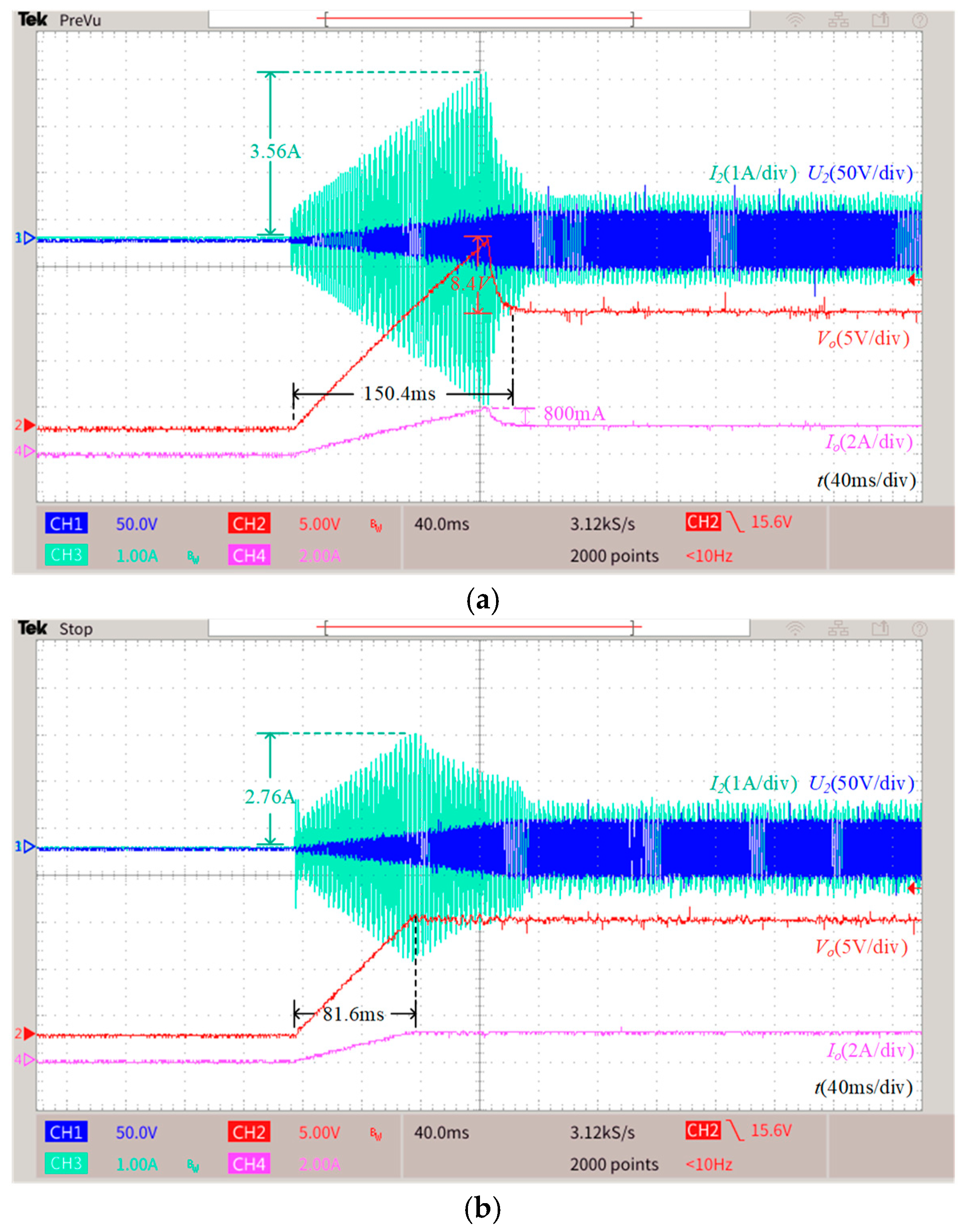
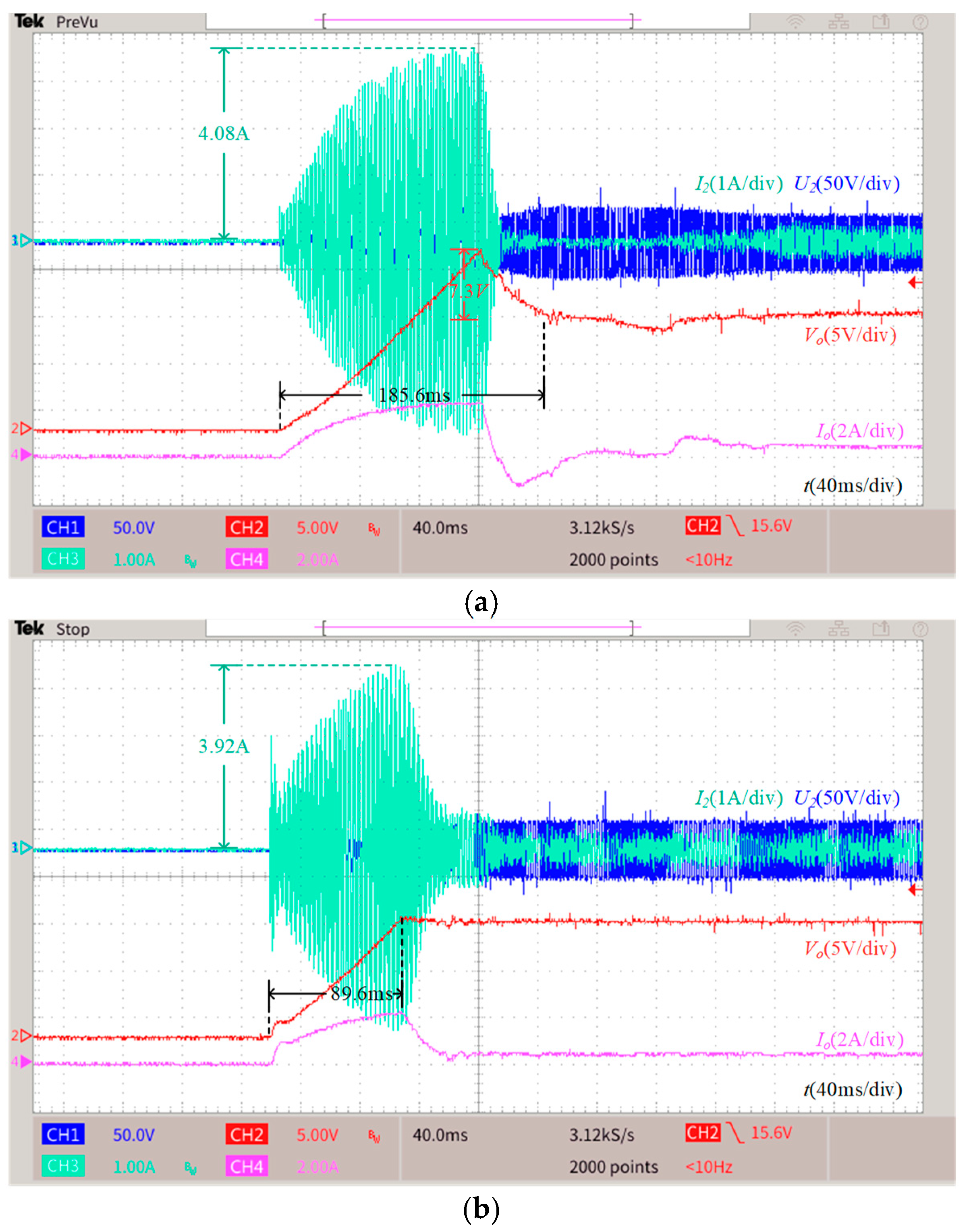
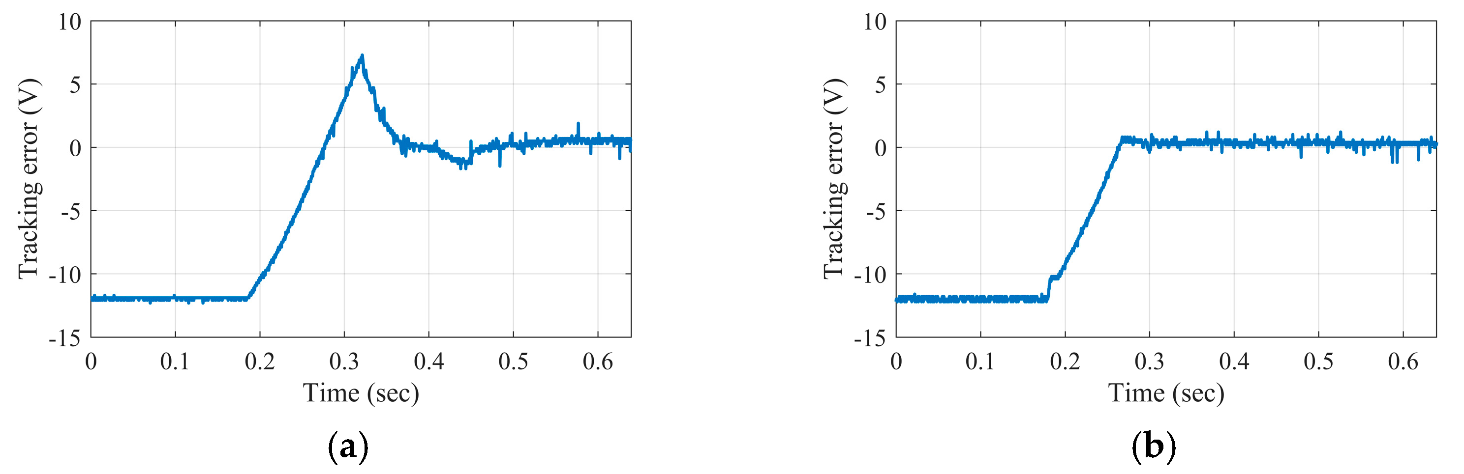
5.2. Case 1: The Start-Up Response

In Case 1, the reference voltage is a constant, namely, $V_d=12 \mathrm{V}$. The experimental results in Case 1 for two control schemes with resistance load and motor load are shown in Figure 4, Figure 5, Figure 6 and Figure 7, respectively. It can be observed clearly that, with resistance load, the proposed FTSM-ELM control achieves significantly superior response performance with settling time (ST) being approximate 81.6 ms, while that of PI control is 150.4 ms. Besides, one can easily notice that a large overshoot 8.4 V appears in PI control, which will inevitably increase the voltage stress in load side. This drawback has been ideally solved by the proposed control scheme. Particularly, a large current overshoot can be seen in the secondary side of the WPT system for the PI control with approximate 3.56 A, while that of the proposed control is only 2.76 A. This feature will reduce the risk of damage to the circuit which ensures the stability of the whole closed-loop system, especially for applications with high power WPT system. From the steady-error point of view, in the period from 350 ms to 640 ms, the proposed control obtains a much smaller root mean square error (RMSE) compared with PI control, with their RMSE values being 0.4240 V and 0.5899 V, respectively. Similar results can be seen with motor load, where the ST of FTSM-ELM control and PI control are 89.6 ms and 185.6 ms, respectively. The RMSE values of FTSM-ELM control and PI control are 0.3960 V and 0.5466 V between 380 ms and 640 ms of steady state. Noticeably, according to the electrical property of the DC motor, with the constant input voltage, the current of the DC motor will decrease when the speed rises. Therefore, there is a current drop with DC motor load exhibited in Figure 6. Since voltage regulation is the primary control target of the proposed control strategy, further analysis of current is omitted here. One might refer to [47] for more details about the electrical property of the DC motor. Besides, it is known that the efficiency varies with different loads [44]. For our application, taking the resistance load 10 Ω, for instance, the overall efficiency is approximately 68.97%. Since the maximum efficiency tracking is not the research task of this paper, the efficiency has not been analyzed in our paper. One can still refer to [44] for more details of maximum power and efficiency tracking issues.

Remark 1.

Notice that the upper-bound settling time$T_f$is independent of the initial values of the system states, but determined by the designed control gains${\alpha }_1$,${\alpha }_2$,$c_1$,$c_2$,$k_1$,$k_2$,$n_1$,$n_2$according to (58). In our application, if we take the component$T_e$and substitute the parameters${\alpha }_1$,${\alpha }_2$,$c_1$,$c_2$, the theoretical convergence time can be obtained as$T_f>T_e=275$ ms. The actual convergence time in our experiment are 81.6 ms and 89.6 ms for resistance and motor load, respectively, which is much smaller than the estimated value of$T_f$. This verifies that the proposed control is capable of achieving a fast dynamic response. It should also be noted that the primary task of theoretical analysis is to illustrate the stability, accuracy and robustness of the proposed control and offer a guide for the controller implementations. And in practical application, the measurement noise in the control loop and sensor is inevitable, which means that the theoretically estimated convergence time is not always exact in the real-time control system.

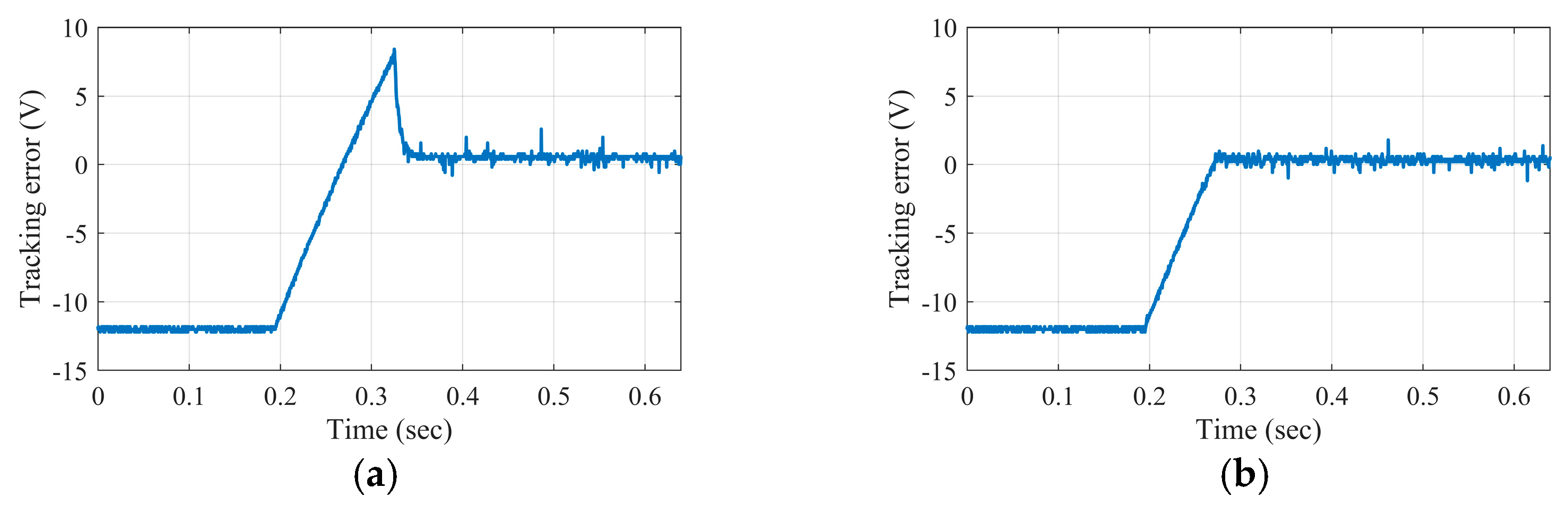
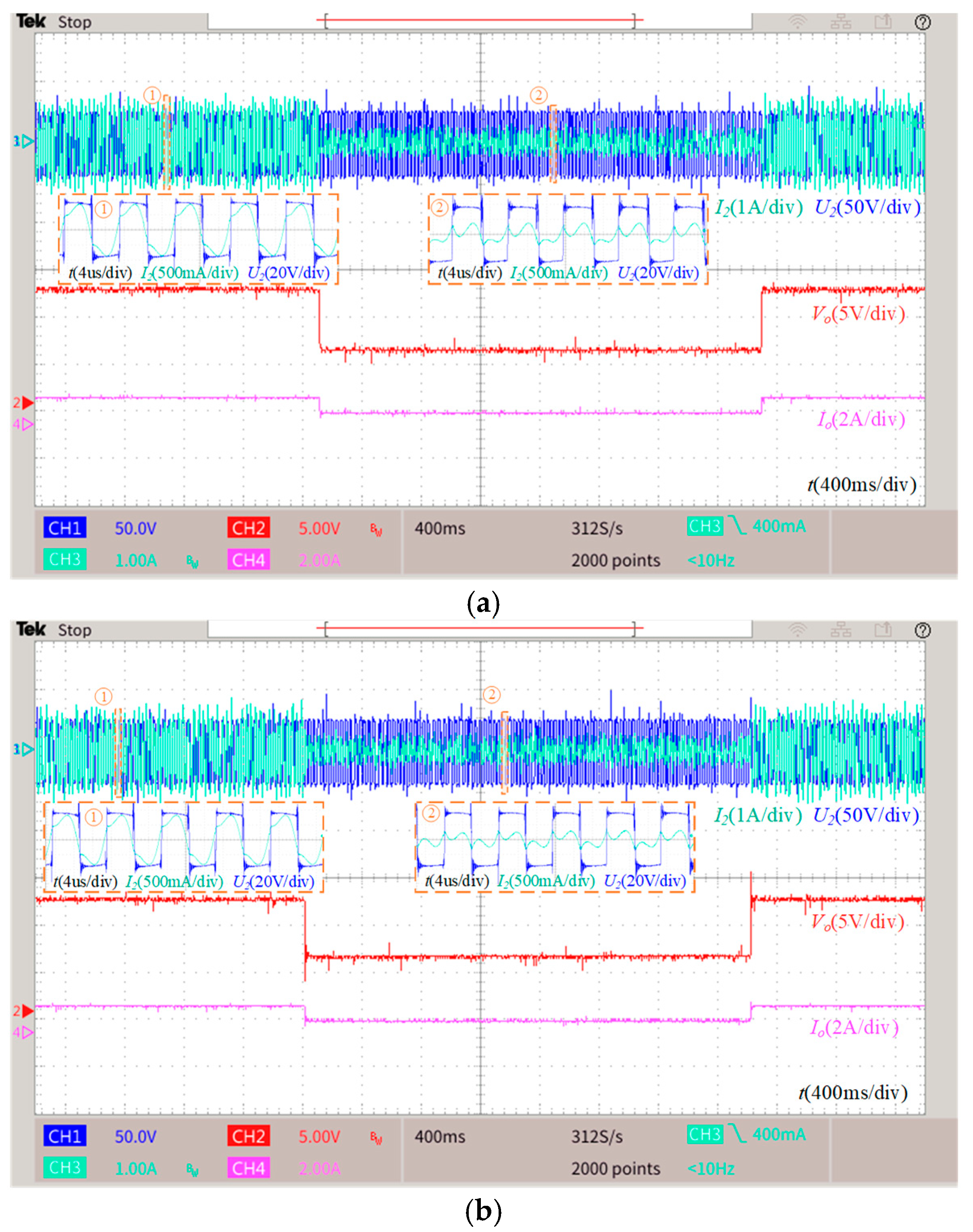
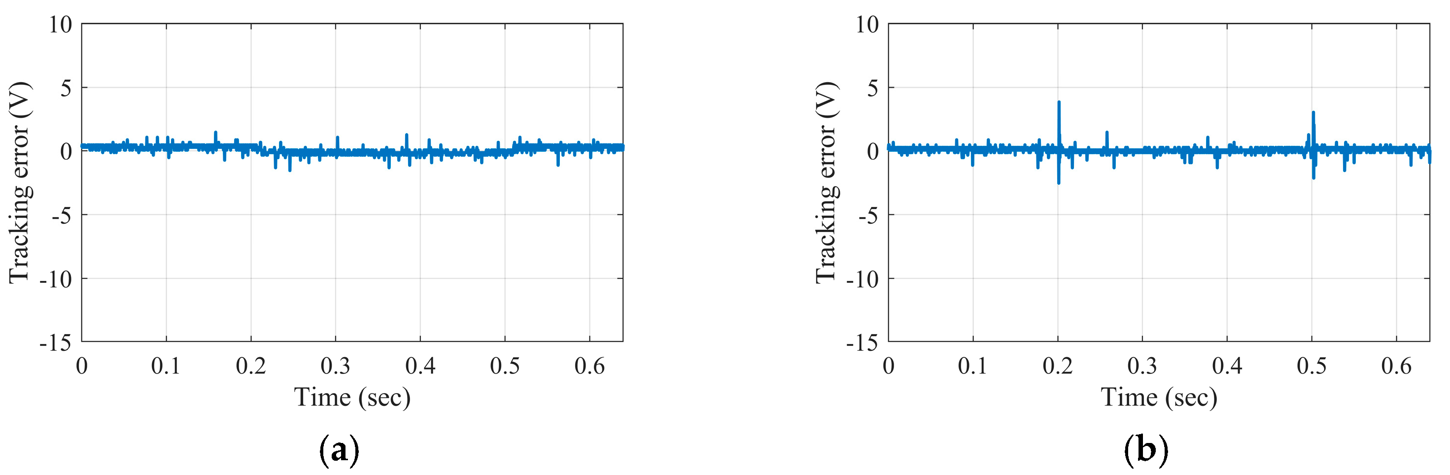
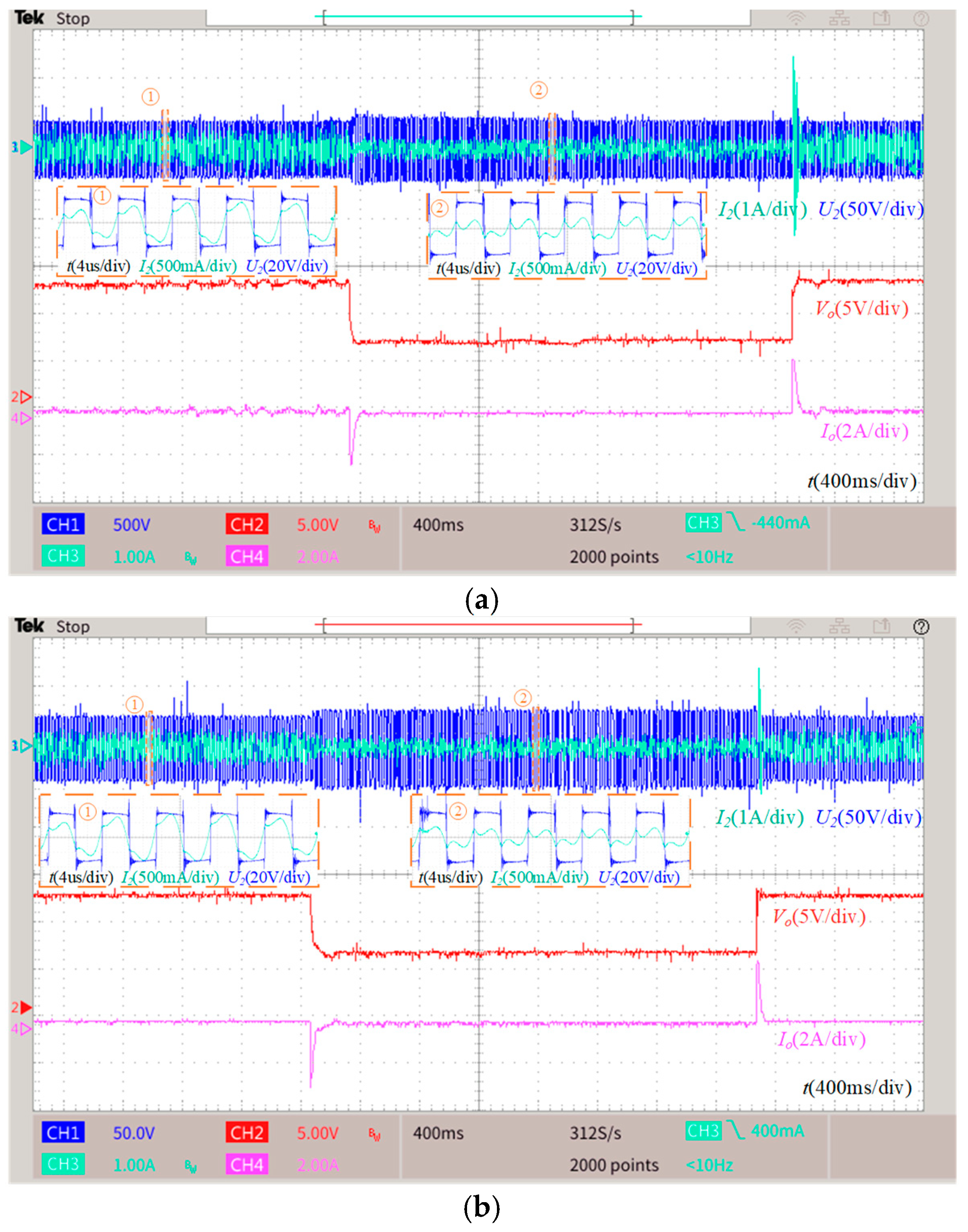
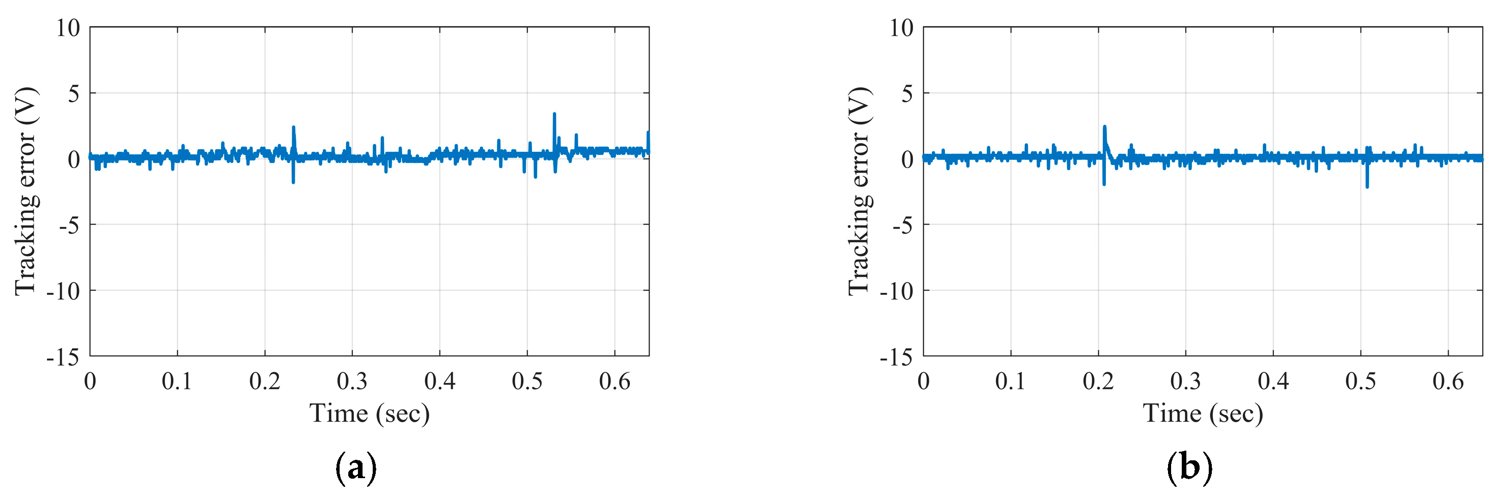
5.3. Case 2: The Set-Point Tracking Performance

In Case 2, the reference voltage is decreased from 12 V to 6 V, then restored back to 12 V. The experiment results in Case 2 for two control schemes with resistance and motor load are shown in Figure 8, Figure 9, Figure 10 and Figure 11, respectively. It is shown vividly that the FTSM-ELM control exhibits better set-point tracking performance with RMSE values of 0.2508 V and 0.2554 V with resistance and DC motor loads, respectively. Comparatively, the RMSE values for PI control are 0.2904 V and 0.4052 V, respectively. The improvement is approximately 13.65% and 36.96% with resistance and DC motor load, respectively. Besides, one might notice from Figure 9 that the proposed control exhibits a relatively large overshoot compared with the PI control when the working condition changes. The reason is that the primary target of the proposed control is to guarantee fast, accurate, and robust voltage tracking performance. Therefore, for achieving a better steady state performance, the control signal will be more aggressive than PI control, which brings a relatively large overshoot in comparison with PI control. However, the overshoot is still within a tolerant range for the WPT applications, and one might also consider the trade-off between overshoot and steady-state performance when determining the parameters of the controller. Furthermore, the secondary voltage and current are shown in the zoomed view of Figure 8 and Figure 10 with resistance and DC motor loads, respectively. It should be noted that the secondary current distorts due to the nonlinearity introduced by buck converter and DC motor load, although the system works in resonance condition. The reasons for the superiority of the FTSM-ELM control can be illustrated in the following facts: (1) The linear structure of PI cannot fully compensate for the nonlinear dynamics in WPT-buck system. Therefore, a large control signal is required to deal with the variations of operation conditions. (2) For the proposed control scheme, due to the introduction of a fast nonlinear sliding manifold, the system error states enjoy a finite time convergence property where the convergence time is independent of the initial values of states. (3) Compared with traditional SMC implementations, an ELM uncertainty upper-bound estimator is further incorporated into the proposed closed-loop WPT-buck control system. As such, the variations of the closed-loop system can be learned in real-time and compensated. In addition, the proposed control innovatively achieves a fixed time convergence for the output weights of ELM to their optimal final values, which aims to ensure the global stability of the closed-loop system in the Lyapunov sense. (4) A URED is applied to obtain the derivative of the output voltage, which successfully eliminates the effects of mismatched disturbance $d_1$ at the same time. From the experiment results, it can be verified that the proposed control scheme can maintain a fast transient response and precise voltage tracking performance for buck converter in an uncertain WPT system.

To better evaluate the robustness of the proposed control strategy, a misalignment rejection test has also been considered in this paper. We chose the reference voltage as 12 V, and misalignment varied between 0% and 40% with a 5% interval. The RMSE value of the evaluation results is shown in

Table 3. Performance evaluation under different alignments of two coils.

Misalignment (%)	0	5	10	15	20	25	30	35	40
RMSE (V)	0.2904	0.3545	0.3855	0.3220	0.3335	0.3840	0.3059	0.3320	0.2485

. One can easily note that the closed-loop stability is almost invariant to the misalignment, and the RMSE values slightly vary from 0.2485 V to 0.3855 V. This also verifies the robustness of the proposed control strategy.

6. Conclusions

In this paper, an ELM-based robust sliding mode feedback control scheme was designed to regulate the voltage of the buck converter for a WPT system in fixed time with parametric variations and unknown external disturbances. The proposed control strategy consists of an FTSM feedback control and ELM-based uncertainty bound estimator. The FTSM feedback control utilizes a singularity-free fast nonlinear sliding dynamic structure, which ensures a fixed time convergence property. A control-oriented ELM estimator was then designed to adaptively learn the bound of the uncertainty. As such, the information of the upper-bound in WPT-buck system is no longer required for FTSM controller. The stability of the whole closed-loop system was proved based on Lyapunov theory. The superior voltage tracking performance in terms of transient, steady-state property was verified with a real-time WPT-buck system.

References

1. Covic, G.A.; Boys, J.T. Inductive Power Transfer. Proc. IEEE 2013, 101, 1276–1289. [Google Scholar] [CrossRef]
2. Han, W.; Chau, K.T.; Zhang, Z. Flexible Induction Heating Using Magnetic Resonant Coupling. IEEE Trans. Ind. Electron. 2017, 64, 1982–1992. [Google Scholar] [CrossRef]
3. Han, W.; Chau, K.T.; Jiang, C.; Liu, W.; Lam, W.H. High-Order Compensated Wireless Power Transfer for Dimmable Metal Halide Lamps. IEEE Trans. Power Electron. 2020, 35, 6269–6279. [Google Scholar] [CrossRef]
4. Ahmad, A.; Alam, M.S.; Chabaan, R. A Comprehensive Review of Wireless Charging Technologies for Electric Vehicles. IEEE Trans. Transp. Electrif. 2018, 4, 38–63. [Google Scholar] [CrossRef]
5. Li, S.; Mi, C.C. Wireless Power Transfer for Electric Vehicle Applications. IEEE J. Emerg. Sel. Top. Power Electron. 2015, 3, 4–17. [Google Scholar] [CrossRef]
6. Han, W.; Chau, K.T.; Liu, W.; Wang, H.; Hua, Z. Wireless Power and Drive Transfer Using Orthogonal Bipolar Couplers and Separately Excited Modulation. IEEE Trans. Ind. Electron. 2022, 69, 3492–3502. [Google Scholar] [CrossRef]
7. Han, W.; Chau, K.T.; Hua, Z.; Hongliang, P. Compact Wireless Motor Drive Using Orthogonal Bipolar Coils for Coordinated Operation of Robotic Arms. IEEE Trans. Magn. 2022, 58, 8200608. [Google Scholar] [CrossRef]
8. Han, W.; Chau, K.T.; Hua, Z.; Hongliang, P. An Integrated Wireless Motor System Using Laminated Magnetic Coupler and Commutative-Resonant Control. IEEE Trans. Ind. Electron. 2022, 69, 4342–4352. [Google Scholar] [CrossRef]
9. Jiang, J.; Song, K.; Li, Z.; Zhu, C.; Zhang, Q. System Modeling and Switching Control Strategy of Wireless Power Transfer System. IEEE J. Emerg. Sel. Top. Power Electron. 2018, 6, 1295–1305. [Google Scholar] [CrossRef]
10. Yang, Y.; Zhong, W.; Kiratipongvoot, S.; Tan, S.-C.; Hui, S.Y.R. Dynamic Improvement of Series–Series Compensated Wireless Power Transfer Systems Using Discrete Sliding Mode Control. IEEE Trans. Power Electron. 2018, 33, 6351–6360. [Google Scholar] [CrossRef]
11. Gheisarnejad, M.; Farsizadeh, H.; Tavana, M.-R.; Khooban, M.H. A Novel Deep Learning Controller for DC–DC Buck–Boost Converters in Wireless Power Transfer Feeding CPLs. IEEE Trans. Ind. Electron. 2021, 68, 6379–6384. [Google Scholar] [CrossRef]
12. Liu, W.; Kim, J.-M.; Wang, C.; Im, W.-S.; Liu, L.; Xu, H. Power Converters Based Advanced Experimental Platform for Integrated Study of Power and Controls. IEEE Trans. Ind. Inform. 2018, 14, 4940–4952. [Google Scholar] [CrossRef]
13. Xu, Q.; Yan, Y.; Zhang, C.; Dragicevic, T.; Blaabjerg, F. An Offset-Free Composite Model Predictive Control Strategy for DC/DC Buck Converter Feeding Constant Power Loads. IEEE Trans. Power Electron. 2019, 35, 5331–5342. [Google Scholar] [CrossRef]
14. Olalla, C.; Queinnec, I.; Leyva, R.; El Aroudi, A. Robust Optimal Control of Bilinear DC–DC Converters. Control Eng. Pract. 2011, 19, 688–699. [Google Scholar] [CrossRef]
15. Boukerdja, M.; Chouder, A.; Hassaine, L.; Bouamama, B.O.; Issa, W.; Louassaa, K.H. Based Control of a DC/DC Buck Converter Feeding a Constant Power Load in Uncertain DC Microgrid System. ISA Trans. 2020, 105, 278–295. [Google Scholar] [CrossRef] [PubMed]
16. Hafiz, F.; Swain, A.; Mendes, E.M.; Aguirre, L.A. Multiobjective Evolutionary Approach to Grey-Box Identification of Buck Converter. IEEE Trans. Circuits Syst. I Regul. Pap. 2020, 67, 2016–2028. [Google Scholar] [CrossRef] [Green Version]
17. Bouchama, Z.; Khatir, A.; Benaggoune, S.; Harmas, M.N. Design and Experimental Validation of an Intelligent Controller for DC–DC Buck Converters. J. Frankl. Inst. 2020, 357, 10353–10366. [Google Scholar] [CrossRef]
18. Edwards, C.; Spurgeon, S. Sliding Mode Control: Theory and Applications; CRC Press: Boca Raton, FL, USA, 1998. [Google Scholar]
19. Hu, Y.; Wang, H.; He, S.; Zheng, J.; Ping, Z.; Shao, K.; Cao, Z.; Man, Z. Adaptive Tracking Control of an Electronic Throttle Valve Based on Recursive Terminal Sliding Mode. IEEE Trans. Veh. Technol. 2021, 70, 251–262. [Google Scholar] [CrossRef]
20. Hu, Y.; Wang, H. Robust Tracking Control for Vehicle Electronic Throttle Using Adaptive Dynamic Sliding Mode and Extended State Observer. Mech. Syst. Signal Process. 2020, 135, 106375. [Google Scholar] [CrossRef]
21. Tan, S.-C.; Lai, Y.-M.; Tse, C.-K. Sliding Mode Control of Switching Power Converters: Techniques and Implementation; CRC Press: Boca Raton, FL, USA, 2018. [Google Scholar]
22. Oucheriah, S.; Guo, L. PWM-Based Adaptive Sliding-Mode Control for Boost DC–DC Converters. IEEE Trans. Ind. Electron. 2012, 60, 3291–3294. [Google Scholar] [CrossRef]
23. Zhao, Y.; Qiao, W.; Ha, D. A Sliding-Mode Duty-Ratio Controller for DC/DC Buck Converters With Constant Power Loads. IEEE Trans. Ind. Appl. 2014, 50, 1448–1458. [Google Scholar] [CrossRef] [Green Version]
24. Komurcugil, H. Adaptive Terminal Sliding-Mode Control Strategy for DC–DC Buck Converters. ISA Trans. 2012, 51, 673–681. [Google Scholar] [CrossRef]
25. Komurcugil, H. Non-Singular Terminal Sliding-Mode Control of DC–DC Buck Converters. Control Eng. Pract. 2013, 21, 321–332. [Google Scholar] [CrossRef]
26. Wang, J.; Li, S.; Yang, J.; Wu, B.; Li, Q. Finite-Time Disturbance Observer Based Non-Singular Terminal Sliding-Mode Control for Pulse Width Modulation Based DC–DC Buck Converters with Mismatched Load Disturbances. IET Power Electron. 2016, 9, 1995–2002. [Google Scholar] [CrossRef]
27. Repecho, V.; Masclans, N.; Biel, D. A Comparative Study of Terminal and Conventional Sliding-Mode Startup Peak Current Controls for a Synchronous Buck Converter. IEEE J. Emerg. Sel. Top. Power Electron. 2021, 9, 197–205. [Google Scholar] [CrossRef]
28. Polyakov, A. Nonlinear Feedback Design for Fixed-Time Stabilization of Linear Control Systems. IEEE Trans. Automat. Contr. 2012, 57, 2106–2110. [Google Scholar] [CrossRef] [Green Version]
29. Zuo, Z. Non-singular Fixed-time Terminal Sliding Mode Control of Non-linear Systems. IET Control Theory Appl. 2015, 9, 545–552. [Google Scholar] [CrossRef]
30. Li, H.; Cai, Y. On SFTSM Control with Fixed-Time Convergence. IET Control Theory Appl. 2017, 11, 766–773. [Google Scholar] [CrossRef]
31. Mahdavi, J.; Nasiri, M.R.; Agah, A.; Emadi, A. Application of Neural Networks and State-Space Averaging to DC/DC PWM Converters in Sliding-Mode Operation. IEEE/ASME Trans. Mechatron. 2005, 10, 60–67. [Google Scholar] [CrossRef]
32. Rubaai, A.; Ofoli, A.R.; Burge, L.; Garuba, M. Hardware Implementation of an Adaptive Network-Based Fuzzy Controller for DC–DC Converters. IEEE Trans. Ind. Appl. 2005, 41, 1557–1565. [Google Scholar] [CrossRef]
33. Wai, R.-J.; Shih, L.-C. Adaptive Fuzzy-Neural-Network Design for Voltage Tracking Control of a DC–DC Boost Converter. IEEE Trans. Power Electron. 2012, 27, 2104–2115. [Google Scholar] [CrossRef]
34. Heydari, A. Optimal Switching of DC–DC Power Converters Using Approximate Dynamic Programming. IEEE Trans. Neural Netw. Learn. Syst. 2018, 29, 586–596. [Google Scholar] [CrossRef]
35. Hajihosseini, M.; Andalibi, M.; Gheisarnejad, M.; Farsizadeh, H.; Khooban, M.-H. DC/DC Power Converter Control-Based Deep Machine Learning Techniques: Real-Time Implementation. IEEE Trans. Power Electron. 2020, 35, 9971–9977. [Google Scholar] [CrossRef]
36. Dong, W.; Li, S.; Fu, X.; Li, Z.; Fairbank, M.; Gao, Y. Control of a Buck DC/DC Converter Using Approximate Dynamic Programming and Artificial Neural Networks. IEEE Trans. Circuits Syst. I Regul. Pap. 2021, 68, 1760–1768. [Google Scholar] [CrossRef]
37. Wang, J.; Luo, W.; Liu, J.; Wu, L. Adaptive Type-2 FNN-Based Dynamic Sliding Mode Control of DC–DC Boost Converters. IEEE Trans. Syst. Man Cybern. Syst. 2021, 51, 2246–2257. [Google Scholar] [CrossRef]
38. Rojas-Dueñas, G.; Riba, J.-R.; Moreno-Eguilaz, M. A Deep Learning-Based Modeling of a 270 V to 28 V DC–DC Converter Used in More Electric Aircrafts. IEEE Trans. Power Electron. 2022, 37, 509–518. [Google Scholar] [CrossRef]
39. Huang, G.-B.; Zhu, Q.-Y.; Siew, C.-K. Extreme Learning Machine: Theory and Applications. Neurocomputing 2006, 70, 489–501. [Google Scholar] [CrossRef]
40. Han, F.; Huang, D.-S. Improved Extreme Learning Machine for Function Approximation by Encoding a Priori Information. Neurocomputing 2006, 69, 2369–2373. [Google Scholar] [CrossRef]
41. Hu, Y.; Wang, H.; Cao, Z.; Zheng, J.; Ping, Z.; Chen, L.; Jin, X. Extreme-Learning-Machine-Based FNTSM Control Strategy for Electronic Throttle. Neural Comput. Applic. 2020, 14507–14518. [Google Scholar] [CrossRef]
42. Hu, Y.; Wang, H.; Yazdani, A.; Man, Z. Adaptive Full Order Sliding Mode Control for Electronic Throttle Valve System with Fixed Time Convergence Using Extreme Learning Machine. Neural Comput. Applic. 2021, 1–13. [Google Scholar] [CrossRef]
43. Zhang, J.; Wang, H.; Ma, M.; Yu, M.; Yazdani, A.; Chen, L. Active Front Steering-Based Electronic Stability Control for Steer-by-Wire Vehicles via Terminal Sliding Mode and Extreme Learning Machine. IEEE Trans. Veh. Technol. 2020, 69, 14713–14726. [Google Scholar] [CrossRef]
44. Dai, X.; Li, X.; Li, Y.; Hu, A.P. Impedance-Matching Range Extension Method for Maximum Power Transfer Tracking in IPT System. IEEE Trans. Power Electron. 2018, 33, 4419–4428. [Google Scholar] [CrossRef]
45. Zuo, Z.; Tie, L. Distributed Robust Finite-Time Nonlinear Consensus Protocols for Multi-Agent Systems. Int. J. Syst. Sci. 2016, 47, 1366–1375. [Google Scholar] [CrossRef]
46. Cruz-Zavala, E.; Moreno, J.A.; Fridman, L.M. Uniform Robust Exact Differentiator. IEEE Trans. Autom. Control 2011, 56, 2727–2733. [Google Scholar] [CrossRef]
47. Sang-Hoon, K. Electric Motor Control; Elsevier: Amsterdam, The Netherlands, 2017; ISBN 978-0-12-812138-2. [Google Scholar]
Figure 1. Structure of series–series compensated WPT system.
Energies 16 01016 g001
Figure 2. Control diagram of the proposed control scheme.
Energies 16 01016 g002
Figure 3. Real-time wireless transfer system.
Energies 16 01016 g003
Figure 4. Tracking performance in Case 1 with resistance load, (a) PI control, and (b) FTSM-ELM control.
Energies 16 01016 g004
Figure 5. Output voltage tracking error in Case 1 with resistance load, (a) PI control, and (b) FTSM-ELM control.
Energies 16 01016 g005
Figure 6. Tracking performance in Case 1 with DC motor load, (a) PI control, (b) FTSM-ELM control.
Energies 16 01016 g006
Figure 7. Output voltage tracking error in Case 1 with DC motor load, (a) PI control, (b) FTSM-ELM control.
Energies 16 01016 g007
Figure 8. Tracking performance in Case 2 with resistance load, (a) PI control, and (b) FTSM-ELM control.
Energies 16 01016 g008
Figure 9. Output voltage tracking error in Case 2 with resistance load, (a) PI control, and (b) FTSM-ELM control.
Energies 16 01016 g009
Figure 10. Tracking performance in Case 2 with DC motor load, (a) PI control, and (b) FTSM-ELM control.
Energies 16 01016 g010
Figure 11. Output voltage tracking error in Case 2 with DC motor load, (a) PI control, and (b) FTSM-ELM control.
Energies 16 01016 g011