Abstract
The central components influencing future grid stability in the future are inverters and their controllers. This paper delves into the pivotal role of inverters and their controllers in shaping the future stability of grids. Focusing on grid-supporting inverters, the study utilizes a microgrid test setup to explore their impact on overall grid stability. Employing impedance-based stability analysis with the Nyquist criterion, the paper introduces variations in internal inverter parameters and external grid parameters using pole-zero map considerations. The inverter’s control structure, resembling standard generators with droop control, facilitates the application of grid operators’ knowledge to inverter control. Mathematical insights into stability principles are provided, highlighting the influence of poles related to the phase-locked loop and the strategic placement of additional poles for enhanced stability. Furthermore, the paper evaluates the effects of rotating inertia, revealing that a 50% increase in system inertia can stabilize unstable microgrid behavior, enabling grid-supporting inverters to actively contribute to grid reliability.
1. Introduction
Driven by the pressing need for sustainability and resilience, the energy landscape has undergone a remarkable transformation in its more than 100-year-long history in just the recent few years. More and more, distributed generation (DG) is being installed, changing the core infrastructure of the power grid [1,2]. Converters and their controllers are at the heart of DG, as they provide access to the grid for renewable resources such as solar and wind. However, the power electrical components comprising an inverter also characterize the electrical behavior of the inverter, which is quite different from that of electrical machines. Here most prominently, three different types of inverters are utilized: grid-following inverter, grid-supporting inverter and grid-forming inverter. Essentially, grid-following inverters rely on a stable grid with voltage and frequency specifications. Based on set points, they only generate power by “following” existing grid conditions. A grid-forming inverter has the ability to “form” its own stable voltage and frequency, similar to a normal power plant, when sufficient energy on the DC side is available [3]. Grid-supporting inverters are a subtype of grid-following inverters that use several different control schemes to react to changes in frequency or voltage via their f/P and V/Q loops. In theory, this means that by coupling grid-forming and grid-supporting inverters, all components for working conditions of the power grid are available. The grid-forming inverter offers a stable voltage source, and the grid-supporting inverter stabilizes and responds to changes in load or generation [4].
Yet regarding the grid, this implies a decreasing number of rotating machines within the grid infrastructure and subsequently less available inertia. As a result, it substantially alters the grid strength, hence modifying the behavior of generated active and reactive power, responses to frequency shifts and voltage changes. Of particular interest is the transition period during and after a fault, as well as the methods for checking stability beforehand. If the fundamental drivers for guaranteed stability are identified, the power grid can become more flexible, adaptable and responsive. When studying smaller grid scenarios in detail, findings can be implemented into the large-scale grid operation as well.
Other research has already realized this idea [5,6] and shown that the behavior of so-called microgrids (MG) can be transferred to the general grid [7]. With an MG approach, low grid strength and a low inertia constant are a given, as they are small-scale, self-contained electrical networks, able to operate in a grid-connected mode and in islanded grid operation [6]. During grid-connected mode, the MG is synchronized to a public grid with substantial grid strength, leveraging operational support and security of supply. In islanded grid operation, the MG is alone in generating stable grid conditions to power all the loads in the MG. As this structure is more flexible to small changes, the control strategies of all components play the most important role and dictate the voltage and frequency inside the MG. By using control algorithms as the deciding component for stability, they can be directly integrated with an assessment of concurrent small signal stability, yielding clear, unambiguous and reliable results [8]. In particular, small signal stability is of paramount importance, as transmission system operators are alerted to electromechanical oscillations in order to take preventive or corrective action [9].
There are several approaches mentioned in the scientific community. The linearized model of the system resulting in a state matrix with eigenvalues is probably the most used mathematical method [10]. However, it is prone to uncertainties, results in computational effort often not solvable in real time and cannot respond to the flexibility and variety of a micro grid [11,12]. Other researchers have proposed a systematic approach based on decision trees, where voltage security and transient stability are evaluated [11,13]. It is one of the most used machine learning techniques applied in the power system, but requires the corresponding infrastructure and user knowledge, which tends to make this approach expensive. From a control perspective, impedance-based considerations have been widely adopted in recent years [14,15]. With the ability to predict dynamic behavior in short time frames and easier adoption due to the determinant-based generalized Nyquist criterion, it is an effective stability tool. Yet, some drawbacks can be found with incorrect stability prediction results when using pure inductance models. Such differences in results have also been observed when transmission lines are modeled using only RL parameters and not PI-equivalent circuits [16].
Regarding the control structure of grid-supporting inverters, different droop controllers [17,18] can be used to react to frequency or voltage changes This structure is intended to explain inverters to give an understanding similar to that of rotation generators. Here, many advantages and disadvantages such as a trade-off between voltage regulation and load sharing [19] when using parallel DGs as well as a slowdown of the dynamic response due to required low pass filters for stabilization for active and reactive power [20] and introduced harmonics from non-linear loads [21] are discussed. For most challenges, other research papers introduce solutions, which in most cases are communication-based but are costly in praxis [22,23]. However, most grid operators are not interested in the fine nuances of used controllers but want to be able to draw a conclusion about whether the integration of a DG will cause difficulty for stable operation conditions or not.
Contributions of this paper:
- Fundamental view based on small grid setup with accessible influence parameters:
This paper uses an islanded MG with a voltage-dependent load, a grid-supporting inverter and a generator as the example grid setup for the stability analysis. All cables are modeled with capacitance values to counteract inaccuracies in stability predictions. This provides clear dependencies between control parameters and grid parameters, showing the extent of each influence transparently.
- Further understanding of grid-supporting inverters:
Through small-signal analysis and variation of several parameters of the grid infrastructure, the understanding of the grid-supporting inverter coupled with the already existing grid infrastructure should be enhanced. The grid-supporting inverter is modeled by an outer and an inner loop. The outer loop consists of a proportional integral (PI) controller for frequency regulation in the grid in the f/P loop, similar to control schemes of rotational generators, and a droop control in the V/Q loop as well as low pass filters on the measured frequency and voltage of the phase-locked loop (PLL). In the inner loop, a PI control and a decoupling component are implemented.
- Simple derivation of control algorithms for grid operators:
With the understanding of the effect parameters have on a small scale, grid operators can regulate the grid accordingly and integrate renewable energies in a stable manner.
The rest of the paper is organized as follows: Section 2 will discuss the design, the used parameters and the general behavior of the model. In Section 3, the whole process is repeated in a small-signal domain before the validation and stability are further described in Section 4, followed by the discussion in Section 5.
2. Modeling in a Time Domain
The general grid model is based on the considerations in [16], but the existing connection to the public grid has been replaced by a generator. As a result, the inverter and the load are located in an island network. The overall grid model consists of the following equipment in the arrangement shown below in Figure 1.
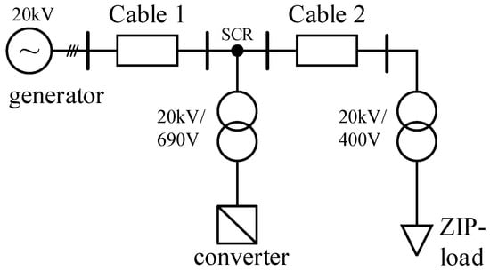
Figure 1.
Test grid system: Island grid situation with grid-supporting inverter.
In general, the medium-voltage network with a line-to-line voltage of 20 kV was maintained. As a grid-supporting inverter is used as a control structure for the inverter in this grid situation, the generator only has to provide a stable phase voltage and phase angle for the inverter’s PLL to control the inverter correctly. This eliminates the need for a complicated equivalent circuit for the generator, allowing the inverter to show its strength in its grid-supporting capabilities. In the time domain simulation, the generator is modeled with transfer functions in the Laplace domain further described in Section 2.1. The generator inertia itself is changed in the model by varying the inertia constant H.
The length of the cable between the generator and the rest of the grid (cable 1) is set to 6 km, and the cable between the inverter and load (cable 2) is fixed to 1 km. As equivalent circuits for the cables, PI models were used with standard parameters of polyethylene cables for medium-voltage grids with a cross section of 120 mm2.
Since the load and the inverter work at line-to-line voltages of 400 V and 690 V, respectively, two transformers with the Dyn vector group are implemented. The usual values for the transformers were utilized.
For the grid-supporting inverter, a rated power of 1 MVA is set at a line-to-line voltage level of 690 V. Based on [16], the structure of the grid-supporting inverter implements droop equations to describe the relationship between f/P and V/Q. However, since a generator is used instead of a grid connection with very high short-circuit power, the droop equation realizing the P/f control is replaced by a PI controller to regulate the error in the grid frequency depending on the power imbalance in the grid system. In Section 2.2, the exact description of the implemented structure is described.
As the equivalent circuit for the load, a polynomial load model is utilized. The general equations from [24] are transformed into a current dependent relationship and implemented using controlled current sources. See [16] for the mathematical process and block diagram. Table 1 describes the utilized parameters of the grid model.

Table 1.
Overview of grid parameters.
2.1. Modeling of Generator
The overall aim for the generator was to produce a stable output voltage. For the sake of clarity, no high-order model was used, but the generator was modeled with the main components that ensure correct operation. For this purpose, the power difference between the turbine power Pturb and the measured power Pgen is calculated as the generator control setpoint, and this difference is then applied to the transfer functions.
The generator model consists of the generator inertia transfer function, the generator system delay transfer function and a static value. From this, the generator frequency is calculated and sent to the three-phase generator, where the grid voltage Vgrid is generated.
The three transfer functions are as follows:
To facilitate comparison of generator inertia with other studies, the generator values are converted to p.u. values within the transfer functions. Here the base value Pbase for the turbine power was set to 1 MW. Figure 2 depicts the block diagram of the generator.
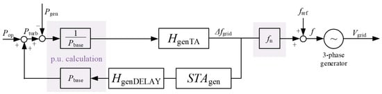
Figure 2.
Block diagram of generator model.
Based on the block diagram, the parameter results are in Table 2.
Table 2.
Generator parameters.
2.2. Modeling of Grid-Supporting Inverter
For the grid-supporting inverter, 1 MVA is used as nominal power with a line-to-line voltage of 690 V. In this model, the inverter is represented using an average model-based voltage source converter. The DC input, typically provided by photovoltaic panels or batteries, is emulated by a DC voltage source supplying twice the rated inverter voltage Vinv,rated for the grid-supporting inverter.
The following control structure is used to obtain the voltage reference signal, depicted in Figure 3: A PLL is used as a synchronization technique. For this, the voltage at the inverter terminals is measured and then transformed via dq transformation to gain the phase angle as well as the PLL frequency used as the reference value for the f/P loop. The same voltage is also transformed via alpha-beta transformation to calculate Vabs as the reference value for the V/Q relation, since alpha-beta transformation depicts better stability than dq transformation [25].
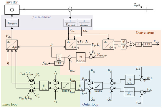
Figure 3.
Block diagram of inverter model.
While the droop equations describing the relationship between f/P and V/Q are the starting point of the control structure of the outer loop, the main goal of the f/P relation of the inverter control is to minimize the error between a reference frequency of 50 Hz and the grid frequency fgrid. Thus the droop equation of the f/P control loop is replaced by a standard PI control with the control values kp,f and ki,f. Another PI control with the control values kp,P and ki,P is implemented, calculating the reference components of the current from the active and reactive power instead of division by the voltage. With the reference currents, the inner loop control, namely the current control, is implemented. Here, another PI control with the control values kp,I and ki,I, similar to other research studies, as well as a decoupling component, is utilized.
Pm and Qm are calculated with the power relation in the alpha-beta domain, following this formula:
Variable as well as set values for the right functionality of the grid-supporting inverter are further described in Table 3. For the controller, fref,inv is converted into a p.u. value.
Table 3.
Grid-supporting inverter parameters.
2.3. Dynamic Investigation of Time Domain Model
To verify the right behavior of the grid model, power jumps are introduced at different times in the generated turbine power and the consumed power of the load. The setpoints P0 and Q0 of the grid-supporting inverter itself are set to zero active and reactive power to check the response of the inverter to the grid events. Stable values for PI control parameters of the grid-supporting inverter are chosen. Here, different techniques for the computation of the control parameters based on calculations of the closed loop transfer function or cut-off frequency with phase margin are used [26].
Test sequence:
- 0 s: Initialization with balanced power values of the grid system, stable after 5 s
- 5 s: Inverter starts
- 15 s: Power increase at load by 0.5 MVA
- 25 s: Power increase at the generator by 0.5 MVA
Description of behavior:
- 0 s: At the start of the simulation, the inverter is off, and the load and generator are initialized at 1 MVA. A small oscillation is observed at both the generator and the load. A positive sign indicates power input (here from the generator), and a negative sign indicates power consumption (here from the load).
- 5 s: The inverter is powered up, and there is a 2 s transient in the power and grid frequency curves. It can be noted that the frequency changes in the 100 mHz range.
- 15 s: At this point, the load increases its consumed power to 1.5 MW. Both the generator and the inverter respond to the power change, although the generator responds faster with a short power peak. This peak is derived from generator inertia, which actually reduces the rotational speed of the generator. Meanwhile, the inverter increases its active power, thus reducing the deficit in active power, and stabilizes the frequency. Since the frequency gradient becomes zero, the power peak of the generator originating from the inertia becomes zero as well. Due to the overshoot in inverter output power, the frequency rises up, and the generator active power counteracts with a reduction and thus drops below 1 MW. Finally, a steady state is reached with the inverter covering the extra load and the generator running with its original set point.Looking directly at the frequency, a maximum reduction of 50 mHz is visible. Due to the inverter’s PI control in the f/P loop, the frequency is not only stabilized but also restored to 50 Hz.
- 25 s: After the system has fully stabilized, the operating point of the generator is now increased to 1.5 MW. The inverter reacts immediately by reducing its output to almost zero. In terms of frequency, this power redistribution has caused a temporary grid frequency increase of 10 mHz.
The test sequence was tried out on the control of the converter in two different ways. First, only the f/P loop was turned on, resulting in the red and black curves in Figure 4. In the second experiment, the V/Q loop was also active, resulting in the black curves in Figure 4. Interestingly, the steady-state behavior of the control is not changed; however, during the switching on of the inverter, the subsequent transient behavior changes significantly. Overshoots and small oscillations can be detected. The so-called coupling between these two control loops is clearly evident, as already described in other research.
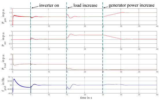
Figure 4.
Power and frequency curves. For the red and blue lines, only the f/P loop was active. For the black lines, the V/Q loop was also active.
3. Modeling in Small-Signal Domain
To gain a better understanding of the influence of control parameters, small-signal methods are the most commonly used analytical methods for evaluation. Since the process is defined for a linear time-invariant system, the model of the system must be based on this consideration. In small-signal modeling, the smallest change around the operating point already indicates an influence on stability. Since network operators want to predict whether a stable grid operation can be maintained, small-signal modeling is the right tool to use. Thus, the whole model is transferred by using the analytical approach and calculating frequency-based transfer functions. The model is developed for the relationship between frequency and active power, which gives the following general correlation:
Based on (3), each part of the grid model is calculated and in the last section put together to obtain the final formula for the small-signal model (SSM).
In (3), ΔP represents the sum of the change of generated and utilized active power of the load, along with the active power jumps that the generator and load performed during the test sequence. Δf describes the change in frequency of the voltage signal that is used for phase angle generation inside the PLL of the grid-supporting inverter and ZIP load.
3.1. Modeling of Generator
To calculate the relationship between frequency and active power of the generator, the block diagram from Figure 2 is used as a basis. From it, the closed loop transfer function is first obtained.
Next, due to the shift in generated turbine power at 25 s, Pturb consists of a constant part and a variable part, , which is now introduced to (4).
By constituting and expanding (5), the transfer function before small-signal modeling is achieved.
For small-signal modeling, all components consisting of constants are set to zero. In this case, this applies to , which leads to the final expression for the frequency expressed as a deviation from the reference frequency for the generator:
Expressed in a block diagram, this results in Figure 5.
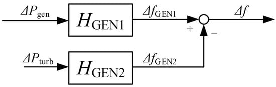
Figure 5.
Block diagram of the SSM of the generator.
3.2. Modeling of Grid-Supporting Inverter
In this paper, the effects of the outer loop of the grid-supported converter are discussed in detail. To achieve this, the small-signal model is developed up to the transition to the inner loop. Normally, outer control loops are developed with lower bandwidth than the inner control loop, resulting in lower cut-off frequencies of low-pass filters as well as slower PI control parameters.
To present the model as a whole, it would be necessary to include the inner loop in the equations [27]. However, as the inner loop usually comprises only a very fast PI controller and a decoupling component, it can be equated to a delay and a constant, which have no major effect on the general behavior of the inverter. In the context of this paper, the current control is accordingly integrated with a delay in the form of 1/s during the calculation.
As a synchronization scheme as well as phase detection, a synchronous reference frame PLL is utilized. This leads to a nonlinear and time-variant model and complicates small-signal modeling. Up to this point, two impedance models, namely one based on the principle of harmonic balance formulated in alpha-beta frame and the other based on the rotating dq frame, have been developed. This paper utilizes the rotating dq frame, comprised of two separate dq frames. By aligning them with the actual grid phase, linearizing the equations and further applying the generalized Nyquist criterion (GNC) to them, the dynamics of the PLL are accounted for. Here, the GNC replaces the standard Nyquist criterion to accommodate a multiple-input and multiple-output system [28].
As a start for the small-signal model of the grid-supporting inverter, the PLL and dq transformation are first performed on the voltage signal. This means that first a Clark and then a Park transformation are applied on the three-phase voltage, reducing it to a two-phase signal.
As input for the PLL, both the d-component and the q-component can be used. In this paper, the focus is on the q-component, which is then compared to Vqref,inv inside the PI controller. However, usage of the q-component introduces a frequency coupling effect in the phase domain, which leads to an asymmetric dq-frame model and makes a decoupling component necessary [27].
From the block diagram, the equations for SSM can be determined, with the PI controller having the following structure: , V = 1 and , corresponding to a first-order Pade function [29].
Expressed in a block diagram, the PLL structure is described in Figure 6.
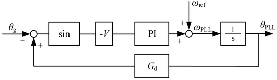
Figure 6.
Block diagram of PLL.
Applying the structure from Figure 6, the following equation for the PLL can be established.
Using linearization methods, the constant components are again set to zero, and the sinusoidal relation turns to 1, simplifying the equation. Further considering the relationship between the phase angle θ and the frequency f with , the equation can be converted to the frequency relation.
The frequency fg is determined by the dq transformation of the voltage component and corresponds consequently to the changing frequency Δf. This relationship can be expressed as
Next, the PI control of the f/P loop is described with the relationship
Two low-pass filters (LPFs) are used in the block diagram of the grid-supporting inverter, namely on the frequency of the PLL fPLL and on the voltage Vabs after alpha-beta transformation.
In s-domain, the LPF is described with the second-order transfer function of (13).
Applying the LPF on the according signals, the frequency of the PLL and the voltage signal for the V/Q loop, the system variables are further refined.
Since all necessary sections have been depicted, the f/P loop equation can be established based on Figure 3.
The saturations of the time domain model were disregarded since small-signal modeling presupposes that there is only a minor deviation from the normal state and that stable behavior can be deduced from this. As such, the signals should not surpass the saturation limits.
Using SSM considerations and inserting (13) and (14), the active power of the inverter is
Expressed in a block diagram, this results in Figure 7.
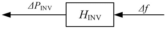
Figure 7.
Block diagram of inverter.
3.3. Modeling of ZIP Load
Regarding the general equation of the ZIP load based on [24], it is depicted that a non-linear behavior occurs. For small-signal modeling, this requires the linearization of the equations of the ZIP load. However, prior to linearizing, the general equation is expanded to account for the low-pass filter.
In addition, a shift in utilized active power usage occurs at 15 s, introducing a constant part and a variable part .
Thus, all components of the equation are included, and the equation can be linearized. For this purpose, the quantities on which there is a dependency are first defined, and then the equation is differentiated according to these quantities.
Quantities with dependencies: ΔPzipload, ΔPzip, Δf.
For easier indication, for all starting parameters, the index “,0” is included. Accordingly, the differentiated equation becomes
In a small-signal domain, the constant value Pzip0 is omitted, and the final equation for the f/P relationship at the ZIP load can be defined.
Expressed in a block diagram, this results in Figure 8.
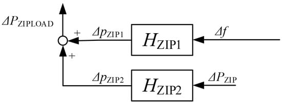
Figure 8.
Block diagram of ZIP load.
3.4. Overall Model in Small-Signal Domain
As a final step, all f/P relations can be summed up and integrated into one equation and one block diagram for better understanding.
First, the equations for the generator are shown in (23).
Next, the equation for the inverter is displayed in (24).
Lastly, the equation for the ZIP load is presented in (25).
Finally, all the equations can be summarized in (26).
Presented in a block diagram, this results in Figure 9.
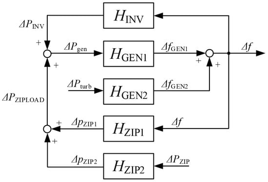
Figure 9.
Block diagram of the complete system.
According to (26), the frequency change depends on two factors: one component influenced by the change in active power consumed by the ZIP load ΔPzip and another component influenced by the change in active power generated by the generator ΔPturb. The inverter is only considered as an influence on the frequency characteristic in the equations and is not a distinct term due to the absence of any specific changes within it. The grid-supporting inverter merely responds to the voltage and frequency of the grid and changes the characteristic by altering its internal behavior, but it does not induce any shift in the grid operation itself. If a grid-forming inverter was used in place of a grid-supporting inverter, the equation would have to include another term describing the influence of the inverter itself. This aligns with the considerations and curves presented in Figure 4.
4. Investigation of the Analytical Model
With the completed analytical model in a small-signal domain, the stability investigation can commence. In particular, the characteristics and influence of the PLL loop is of interest, as different research [15,28,30] describes negative effects in stability due to the PLL and its interaction with the grid impedance. However, as a demonstration of the correct functionality of the analytical equation, the SSM is initially compared to the time-domain model. Subsequently, a study examining the change in pole placement when several parameters are varied is conducted. Building on this knowledge, a three-dimensional volume is created to demonstrate the coupling effects between the two control parameters on stability.
4.1. Validation of the Analytical Model
To test the correct operation of the analytical model, the transfer functions of Section 3.3 are also constructed in Simulink and compared with the time-domain model. A step of −0.2 p.u. was applied at 0.5 s to the nominal power of the generator and the resulting change in ΔPgen observed. In theory, the measured value for the power should therefore change from 1 MW to 0.8 MW.
Figure 10 depicts the time-domain model’s behavior in the blue curve and the small-signal model’s behavior in the red curve. It can be noted that both curves overlap and show the same behavior throughout the step. Both measured powers have accordingly the same time constants and characteristic during the small oscillation when the step is introduced. The overall value also significantly drops from 1 MW to 0.8 MW as intended. This validation demonstrates that the analytical model can be effectively used as an analytical representation of the time-domain simulation, and the stability investigation can proceed.
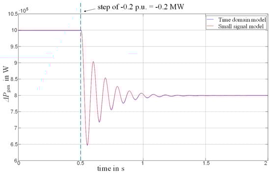
Figure 10.
Step response of the complete system.
4.2. Stability Investigation
As per the final equation of the small-signal model, (26), it is possible to consider the behavior resulting from the change of the generated generator power and from the consumed power of the load separately. For stability analysis, various methods can be used, but the general Nyquist criterion (GNC) is typically preferred. The reason is, as mentioned above in Section 3.2, the transformation of the synchronous reference frame PLL to a stationary reference frame, which changes the characteristic of the system from a single-input and single-output system to a multiple-input and multiple-output system. This means that the standard Nyquist criterion is no longer sufficient for stability analysis, and the GNC is necessary for an accurate assessment of the system.
In this section, first, the stability of the system depending on the grid-supporting inverter with different values for the PI controller of the f/P loop, which represents the frequency tuning component, is varied, and secondly, the inertia of the generator is varied.
4.2.1. Stability Depending on the Variation of the PI Controller
If the general Nyquist criterion (GNC) is used as a stability criterion and represented by the real and imaginary components of the transfer function, the stability depends on the sum of the characteristic loci encircling the critical point (−1 + j0) in a counterclockwise direction. In other words, the occurrence of poles on the right half plane (RHP) indicates unstable performance of the entire system. To determine whether such behavior occurs, different visualization techniques can be utilized. In this paper, a pole-zero plot describes the behavior of the poles during the variation of the components. By assigning each set of poles a distinct color and arranging the values in ascending order, the behavior can be observed very clearly. Commencing with the color pink denoting the lowest values, the results transition progressively towards the color yellow as the values increase.
For Figure 11, kp,f was varied between 200 and 1000, ki,f was varied between 500 and 100,000 and the generator inertia H was set to 2.
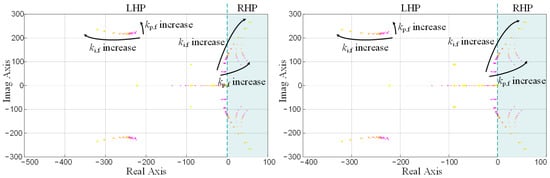
Figure 11.
Pole zero plot of small-signal model, PI controller varied. (Left) Component dependent on generator change. (Right) Component dependent on load change.
Upon initial inspection, it becomes apparent that the system exhibits not only a singular pair of poles but encompasses multiple poles that closely resemble each other in both transfer functions. This is explained by the shared mathematical relationship; the system is a 35th-order function for the component that depends on the load shift and a 24th-order function for the component that depends on the generator power change.
Upon further examination of the type of poles in the system, different types can be described:
- Poles with only real components (σ + j0):When located on the left half plane (LHP), these poles depict an exponentially decaying component in the time domain. Here, the location of the pole determines the rate of decay, with poles located further away from the origin, leading to faster decay rates. Therefore, poles far from the origin are components offering the transfer function quick stabilization to a settled value. If a real pole was to appear on the right half of the plane (RHP), it would correspond to an exponentially increasing component and render the system unstable.
- Poles with an imaginary component, which appear as complex conjugated poles (σ + j ω):Complex conjugated poles located in the LHP lead to a decaying sinusoidal component in the time domain. Again, the rate of decay is determined by the location of the real part of the pole σ, while the frequency of the sinusoidal oscillation is determined by ω. Vice versa, complex conjugate poles in the RHP result in an increasing sinusoidal component in the time domain, leading to an oscillation that continually increases, making the system unstable.
- Poles at the origin (0 + j0):These poles result in a constant that is determined by the initial values. Here, the set values are P0, Q0, Vref and fref of the inverter.
In general, with selected stable values, the system consists accordingly of different exponentially decaying components and decaying sinusoidal components. When compared to Figure 10, where a small step signal was applied to the stable system, this behavior can be observed. Further, [16] also confirms that with an increase of the proportional and integral part of the PI controller of the f/P loop with the controller values kp,f and ki,f, unstable behavior occurs.
If further viewed on a two-dimensional plot with a stability index, distinct boundaries can be observed between the stable and unstable regions. The analytical model’s equation was used to vary the control parameters and identify the poles for each system. Any pole in the RHP was recorded as an unstable state, while absence of a pole in the RHP was noted as a stable state. In Figure 12, the dark blue represents the stable values of the controller values, and the yellow area represents the unstable values. The x-axis describes the control parameter kp,f, while the y-axis displays ki,f. Again, when compared with the results from [16], the regions in the plots of stability index are very similar. This means that whether a public grid connection or a generator with separately adjustable inertia is utilized, higher PI controller values lead to system instability.
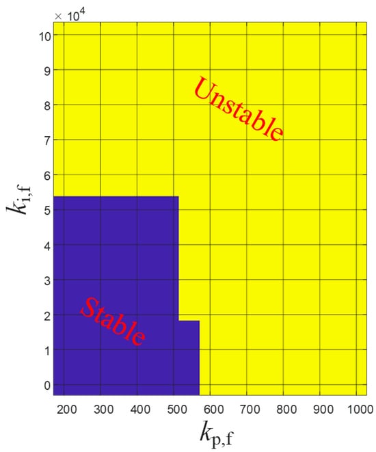
Figure 12.
Stability index plots.
The transfer functions of both parts of (26) were compared, revealing negligible disparities. Consequently, for enhanced clarity, only one plot is presented. This finding substantiates the hypothesis that alterations in a specific component influence the entire system, attributing it to the shared mathematical relationships.
4.2.2. Stability Depending on the Variation of the Generator Inertia
In this investigation of stability, the focus was on the rate of pole transition from stable to unstable behavior according to GNC. For this reason, unstable values of kp,f and ki,f were selected for investigation to determine whether unstable behavior can be transformed into stable behavior simply by increasing generator inertia. Since the dynamic influence of the grid-supporting inverter should diminish with a large amount of inertia in the system, this notion can be feasible. In general, it can be assumed that the stability of the entire system improves with higher values of inertia.
For Figure 13, H was varied between 1 and 20 in increments of 1, while the PI controller values were set to kp,f = 1000 and ki,f = 800.
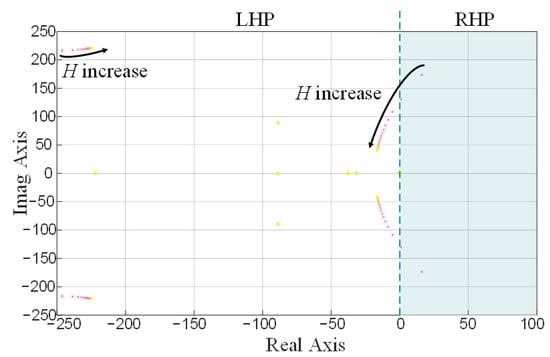
Figure 13.
Pole-zero plot of small-signal model, generator inertia varied.
The system includes various types of poles that correspond to the types of poles shown in Figure 11.
- Poles with only real components (σ + j0)
- Poles with an imaginary component, which appear as complex conjugated poles (σ + j ω)
- Poles at the origin (0 + j0)
As expected, high inertia values lead to stable system behavior. It is apparent that the poles rapidly migrate to the left-hand plane and the system remains stable for values of H greater than or equal to 3. Thus, the initial suggestion that the power grid can only consist of grid-supporting and grid-following inverters is only possible if at least significant inertia in relation to the grid impedance is present in the system.
4.2.3. Visualization in a 3D Plot
To gain better understanding of the dependences of kp,f, ki,f with regard to H, the stability index was set up as a function of all three parameters. If an unstable behavior was detected on the RHP, a value of 1 was assigned in the stability matrix. If no unstable behavior was found, a value of 0 was entered in the stability matrix.
Figure 14 describes the behavior, where the area in red represents the unstable area of the system. For the plot kp,f ranging from 200 to 1200, ki,f varied between 500 and 10,000, and H was in the range of 1 to 10.
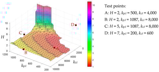
Figure 14.
3D plot of stability matrix as a function of kp,f, ki,f and H.
In Figure 14, the surface between the stable and unstable areas is plotted. All values above the surface are stable, and all values below are unstable. As can be observed, at higher values of H, the region of unstable control parameters decreases gradually. The difference in H required to shift from the stable to the unstable area is often minimal. In many cases, increasing the inertia constant from 2 to 3 is enough to convert an unstable system to a stable one. These findings are valuable for grid operators, as in those cases, increasing half of the rotating inertia in the grid enables inverters to support grid operation. Additionally, the plot reveals that kp,f significantly impacts stability more than ki,f. This is reasonable since a signal can be influenced much more efficiently with the proportional component than with the integral component. A detailed comparison of the two control parameters further corroborates: If kp,f exceeds a certain value, regardless of how high the generator inertia constant is set, the entire system will remain unstable. In short, setting kp,f completely wrong will not allow the generator inertia to restore system stability. It can be concluded that the system will remain unstable if the generator inertia is less than 1. Increasing the inertia constant also extends the range of possible values for kp,f and ki,f.
4.2.4. Time Domain Validation
As a final step, a number of points are selected from Figure 13 and compared to the time-domain simulation. By selecting a point within the stable region based on the stability index, stable behavior should be exhibited in the time domain and vice versa with an unstable point.
Figure 14 displays the selected test points A, B, C and D, while Figure 15 presents the corresponding results of the time domain simulation.
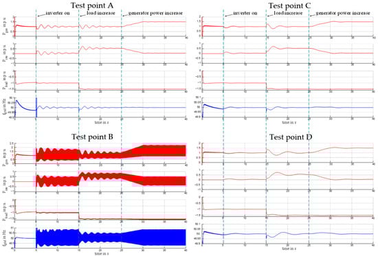
Figure 15.
Time domain analysis of test points.
According to Figure 14, test points A and B are expected to demonstrate stable behavior, while points C and D are expected to display unstable behavior in the time domain.
Figure 15 corresponds closely with the findings from the stability indexing analysis in Figure 14. Notably, test points A and B also display unstable curves concerning effective powers and frequency in the time domain simulation. This study establishes that the unstable behavior has various outcomes. While test point A produces slow oscillation with low amplitude lasting for over 10 s, at most 0.25 p.u. larger than the nominal state, test point B yields rapid oscillation with high amplitude, at most 1 p.u. larger than in the nominal state. Test points C and D generate stable curves that quickly stabilize. The switching times remain unchanged from Section 2.3.
5. Discussion
Understanding the behavior of grid-supporting inverters is essential for grid operators. Stability is a direct outcome of the interaction between the existing grid impedance and the control mechanism of the inverter. For this reason, an MG setup was utilized to address potential instabilities from the triggering parameter.
Findings are summarized as followed:
- The assumption that both the grid and inverter could impact microgrid stability was validated. Changes in grid parameters and inverter control parameters were identified as potential destabilizing factors.
- Initially, a grid-supporting inverter was mathematically derived using small-signal modeling and the corresponding transfer function. The importance of applying the generalized Nyquist criterion to multi-input and multi-output systems was emphasized, revealing the significant role of pole type in subsequent behavior.
- Stability is notably influenced by the PLL, expressing poles with imaginary parts, typically as complex conjugated pole pairs. This study explores additional types of poles that positively affect the converter’s behavior based on their location on the LHP, following the generalized Nyquist criterion.
- The system’s stability is notably influenced by the value of kp,f, as indicated by the analytical study. Exceeding 518 in this grid system renders the system unstable, even with increased generator inertia. High ki,f values affect the oscillation behavior of the output signal, with simulations indicating 5000 as a limit, beyond which slow, decreasing oscillations occur. A significant discrepancy is observed when comparing these values with control values of rotating generators, being hundreds of times larger. This underscores the need for grid operators to expand their knowledge to effectively control a grid heavily influenced by inverters.
- The evaluation of rotating inertia showed that increasing it can convert unstable microgrid behavior into stability by shifting poles. A noteworthy finding is that an increase in inertia (0.5 to 1 p.u.) is often sufficient for stability, enabling active participation of the inverter in grid operation. However, when scaled to the entire European grid, this proportion becomes impractical, requiring a significant contribution from rotating generators at some point.
Finally, the paper suggests the following first draft of a step-by-step guide for grid operators before connecting a renewable source:
- Evaluation of grid impedance and visualization in a pole zero map
- Evaluation of inverter impedance and visualization in a pole zero map
- Comparison of inverter impedance poles with grid impedance poles. In case poles of the inverter system alone are already on the RHP, compensation mechanisms must be applied, or poles must be shifted with the control parameters. Should the combination of poles result in poles on the RHP, the inverter control parameters should be changed.
Author Contributions
Conceptualization, C.L.; methodology, C.L.; software, C.L.; validation, C.L.; formal analysis, C.L. and Z.Z.; investigation, C.L.; writing—original draft preparation, C.L.; writing—review and editing, C.L., Z.Z., H.R. and R.S.; visualization, C.L.; supervision, H.R. and R.S.; project administration, C.L. All authors have read and agreed to the published version of the manuscript.
Funding
Supported by the Graz University of Technology Open Access Publishing Fund.
Data Availability Statement
Data are contained within the article.
Acknowledgments
Graz University of Technology Open Access Publishing Fund.
Conflicts of Interest
The authors declare no conflict of interest.
References
- Sahoo, A.K.; Mahmud, K.; Crittenden, M.; Ravishankar, J.; Padmanaban, S.; Blaabjerg, F. Communication-Less Primary and Secondary Control in Inverter-Interfaced AC Microgrid: An Overview. IEEE J. Emerg. Sel. Top. Power Electron. 2021, 9, 5164–5182. [Google Scholar] [CrossRef]
- Gui, Y.; Nainar, K.; Bendtsen, J.D.; Diewald, N.; Iov, F.; Yang, Y.; Blaabjerg, F.; Xue, Y.; Liu, J.; Hong, T.; et al. Voltage Support with PV Inverters in Low-Voltage Distribution Networks: An Overview. IEEE J. Emerg. Sel. Topics Power Electron. 2023, 1. [Google Scholar] [CrossRef]
- Rocabert, J.; Luna, A.; Blaabjerg, F.; Rodríguez, P. Control of Power Converters in AC Microgrids. IEEE Trans. Power Electron. 2012, 27, 4734–4749. [Google Scholar] [CrossRef]
- Zhang, Z.; Lehmal, C.; Hackl, P.; Schuerhuber, R. Transient Stability Analysis and Post-Fault Restart Strategy for Current-Limited Grid-Forming Converter. Energies 2022, 15, 3552. [Google Scholar] [CrossRef]
- Lin, Q.; Uno, H.; Ogawa, K.; Kanekiyo, Y.; Shijo, T.; Arai, J.; Matsuda, T.; Yamashita, D.; Otani, K. Field Demonstration of Parallel Operation of Virtual Synchronous Controlled Grid-Forming Inverters and a Diesel Synchronous Generator in a Microgrid. IEEE Access 2022, 10, 39095–39107. [Google Scholar] [CrossRef]
- Zhong, Q.-C.; Weiss, G. Synchronverters: Inverters that mimic synchronous generators. IEEE Trans. Ind. Electron. 2011, 58, 1259–1267. [Google Scholar] [CrossRef]
- Sandelic, M.; Peyghami, S.; Sangwongwanich, A.; Blaabjerg, F. Reliability aspects in microgrid design and planning: Status and power electronics-induced challenges. Renew. Sustain. Energy Rev. 2022, 159, 112127. [Google Scholar] [CrossRef]
- Zhang, Z.; Schuerhuber, R.; Fickert, L.; Friedl, K. Study of stability after low voltage ride-through caused by phase-locked loop of grid-side converter. Int. J. Electr. Power Energy Syst. 2021, 129, 106765. [Google Scholar] [CrossRef]
- Zanjani, M.G.M.; Mazlumi, K.; Kamwa, I. Combined analysis of distribution-level PMU data with transmission-level PMU for early detection of long-term voltage instability. IET Gener. Transm. Distrib. 2019, 13, 3634–3641. [Google Scholar] [CrossRef]
- Kundur, P.; Paserba, J.; Ajjarapu, V.; Andersson, G.; Bose, A.; Canizares, C.; Hatziargyriou, N.; Hill, D.; Stankovic, A.; Taylor, C.; et al. Definition and Classification of Power System Stability IEEE/CIGRE Joint Task Force on Stability Terms and Definitions. IEEE Trans. Power Syst. 2004, 19, 1387–1401. [Google Scholar] [CrossRef]
- da Cunha, G.L.; Fernandes, R.A.; Fernandes, T.C.C. Small-signal stability analysis in smart grids: An approach based on distributed decision trees. Electr. Power Syst. Res. 2022, 203, 107651. [Google Scholar] [CrossRef]
- Zhang, J.; Chung, C.Y.; Wang, Z.; Zheng, X. Instantaneous Electromechanical Dynamics Monitoring in Smart Transmission Grid. IEEE Trans. Ind. Inform. 2016, 12, 844–852. [Google Scholar] [CrossRef]
- Liu, C.; Sun, K.; Rather, Z.H.; Chen, Z.; Bak, C.L.; Thogersen, P.; Lund, P. A Systematic Approach for Dynamic Security Assessment and the Corresponding Preventive Control Scheme Based on Decision Trees. IEEE Trans. Power Syst. 2014, 29, 717–730. [Google Scholar] [CrossRef]
- Qiao, L.; Xue, Y.; Kong, L.; Wang, F. Nodal Admittance Matrix Based Area Partition Method for Small-Signal Stability Analysis of Large-Scale Power Electronics Based Power Systems. In Proceedings of the 2021 IEEE Applied Power Electronics Conference and Exposition (APEC), Phoenix, AZ, USA, 14–17 June 2021. [Google Scholar]
- Qiao, L.; Xue, Y.; Kong, L.; Wang, F. A Potential Issue of Using the MIMO Nyquist Criterion in Impedance-Based Stability Analysis. IEEE Open J. Power Electron. 2022, 3, 899–904. [Google Scholar] [CrossRef]
- Lehmal, C.; Zhang, Z.; Renner, H.; Schürhuber, R. Requirements for grid supporting inverter in relation with frequency and voltage support. In Proceedings of the CIRED 2023: 27th International Conference & Exhibition on Electricity Distribution, Rome, Italy, 12–15 June 2023; Available online: https://www.cired2023.org/ (accessed on 7 December 2023).
- Simpson-Porco, J.W.; Dörfler, F.; Bullo, F. Synchronization and power sharing for droop-controlled inverters in islanded microgrids. Automatica 2013, 49, 2603–2611. [Google Scholar] [CrossRef]
- Zhong, Q.-C. Robust Droop Controller for Accurate Proportional Load Sharing Among Inverters Operated in Parallel. IEEE Trans. Ind. Electron. 2013, 60, 1281–1290. [Google Scholar] [CrossRef]
- Yang, N.; Paire, D.; Gao, F.; Miraoui, A.; Liu, W. Compensation of droop control using common load condition in DC microgrids to improve voltage regulation and load sharing. Int. J. Electr. Power Energy Syst. 2015, 64, 752–760. [Google Scholar] [CrossRef]
- Guerrero, J.; GarciadeVicuna, L.; Matas, J.; Castilla, M.; Miret, J. A Wireless Controller to Enhance Dynamic Performance of Parallel Inverters in Distributed Generation Systems. IEEE Trans. Power Electron. 2004, 19, 1205–1213. [Google Scholar] [CrossRef]
- Alsafran, A. Literature Review of Power Sharing Control Strategies in Islanded AC Microgrids with Nonlinear Loads. In Proceedings of the 2018 IEEE PES Innovative Smart Grid Technologies Conference Europe (ISGT-Europe), Sarajevo, Bosnia and Herzegovina, 21–25 October 2018. [Google Scholar]
- Arbab-Zavar, B.; Palacios-Garcia, E.J.; Vasquez, J.C.; Guerrero, J.M. Smart Inverters for Microgrid Applications: A Review. Energies 2019, 12, 840. [Google Scholar] [CrossRef]
- Nutkani, I.U.; Loh, P.C.; Wang, P.; Blaabjerg, F. Autonomous Droop Scheme With Reduced Generation Cost. IEEE Trans. Ind. Electron. 2014, 61, 6803–6811. [Google Scholar] [CrossRef]
- Kundur, P. Power System Stability and Control; McGraw-Hill: New York, NY, USA, 1998. [Google Scholar]
- Ahmad, S.; Mekhilef, S.; Mokhlis, H. An improved power control strategy for grid-connected hybrid microgrid without park transformation and phase-locked loop system. Int. Trans. Electr. Energy Syst. 2021, 31, e12922. [Google Scholar] [CrossRef]
- Joseph, S.B.; Dada, E.G.; Abidemi, A.; Oyewola, D.O.; Khammas, B.M. Metaheuristic algorithms for PID controller parameters tuning: Review, approaches and open problems. Heliyon 2022, 8, e09399. [Google Scholar] [CrossRef] [PubMed]
- Wang, X.; Harnefors, L.; Blaabjerg, F. Unified Impedance Model of Grid-Connected Voltage-Source Converters. IEEE Trans. Power Electron. 2018, 33, 1775–1787. [Google Scholar] [CrossRef]
- Gu, Y.; Zhu, R.; Qi, X.; Wu, W.; Aini, H.; Chang, X. Small-Signal Impedance-based Stability Analysis of Self-Synchronizing Grid-Following Converters. In Proceedings of the 2022 IEEE International Power Electronics and Application Conference and Exposition (PEAC), Guangzhou, China, 4–7 November 2022. [Google Scholar]
- Bequette, B.W. Process Control: Modeling Design and Simulation; Prentice-Hall of India Private Limited: New Delhi, India, 2006. [Google Scholar]
- Wen, B.; Boroyevich, D.; Mattavelli, P.; Shen, Z.; Burgos, R. Influence of phase-locked loop on dq frame impedance of three-phase voltage source converters and the impact on system stability. In Proceedings of the 2013 Twenty-Eighth Annual IEEE Applied Power Electronics Conference and Exposition (APEC), Long Beach, CA, USA, 17–21 March 2013; pp. 897–904. [Google Scholar] [CrossRef]
Disclaimer/Publisher’s Note: The statements, opinions and data contained in all publications are solely those of the individual author(s) and contributor(s) and not of MDPI and/or the editor(s). MDPI and/or the editor(s) disclaim responsibility for any injury to people or property resulting from any ideas, methods, instructions or products referred to in the content. |
© 2023 by the authors. Licensee MDPI, Basel, Switzerland. This article is an open access article distributed under the terms and conditions of the Creative Commons Attribution (CC BY) license (https://creativecommons.org/licenses/by/4.0/).