Optimizing the Controlling Parameters of a Biomass Boiler Based on Big Data

Abstract

This paper presents a comprehensive method for optimizing the controlling parameters of a biomass boiler. The historical data are preprocessed and classified into different conditions with the k-means clustering algorithm. The first-order derivative (FOD) method is used to compensate for the lag of controlling parameters, the backpropagation (BP) neural network is used to map the controlling parameters with the boiler efficiency and unit load, and the ant colony optimization (ACO) algorithm is used to search the opening of air dampers. The results of the FOD-BP-ACO model show an improvement in the boiler efficiency compared to the predicted values of FOD-BP and the data compared to the historical true values were observed. The results suggest that this FOD-BP-ACO method can also be used to search and optimize other controlling parameters.

1. Introduction

As a renewable energy, biomass energy is drawing a lot of attention around the world. The installed biomass power energy capacity has exceeded 120 GW (as shown in Figure 1) [1].

Figure 1. The total installed capacity of global biomass power generation from 2012 to 2021 [1].

To improve the efficiency of the plant, the big data analysis method was attempting to optimize the operation of the boiler. Li et al. [2] proposed an artificial neural network (ANN) and showed better regression accuracy and generalization ability with faster learning speed. Krzywanski et al. [3,4] built a feedforward ANN to predict SO₂ emissions. Gao et al. [5] proposed a method based on improved particle swarm (HPSO) and support vector machine (SVM) algorithms for the prediction of the NOx concentration in flue gas. Li et al. [6] used the Lasso algorithm of machine learning to conduct a correlation analysis of boiler control parameters and operating state parameters, and extracted highly correlated control parameters and operating state parameters. A nonlinear combined deep confidence network (NCDBN) was used to predict the exhaust gas’s boiler efficiency and NOx content.

L. D. Blackburn [7] proposed a constrained dynamic optimization using a recurrent neural network model combined with a meta-heuristic optimizer. An improvement was achieved for the simulated coal-fired boiler compared to the non-optimal situation. Yao et al. [8] proposed an ANN model to improve the unit heat rate by optimizing the boiler load, boiler excess oxygen (O₂), fly ash unburned carbon, and descaling flow rate for coal-fired boilers.

Wei Tian and Yu Cao proposed an innovative study where they optimized the backpropagation (BP) neural network based on the firefly algorithm (FA). They also introduced the sparrow search algorithm (SSA), altering the search mechanism of BP to address the issue of local optima affecting traditional BP [9].

However, the above studies do not consider the large inertia of boiler parameters. Delays in predicting parameters may hinder the ability to take timely corrective actions and lead to suboptimal performance.

Hence, this study considers the effect of delay parameter compensation, and an FOD-BP-ACO model is proposed. The individual steps for the optimization of control parameters are summarized as follows:

Step I: Data cleaning with the PauTa criterion and classification with the k-means method.

Step II: Parameter selection with the average impact value (AIV) method.

Step III: Compensating the lag of controlling parameters with the first-order derivative (FOD) method.

Step IV: Modeling with backpropagation (BP) neural networks and random forest.

Step V: Optimizing the opening of the air damper through the ant colony algorithm.

The biomass direct-fired 130 t/h (9.2 MPa and 540 °C) boiler structure diagram is showed in Figure 2 and all the used data are collected from this power plant.

Figure 2. Simplified diagram of the biomass boiler.

2. Materials and Methods

2.1. Data Processing and Analysis

Boiler operational data frequently exhibit anomalies due to various sources of interference, such as noise, sensor malfunctions, abnormal operational conditions, system instability, and other factors. It is necessary to assess the reliability of the measurement data [10].

(1) Data cleaning

The threshold of 3$\sigma$-based PauTa [11] criterion is used as the outlier detection method. The standard deviation is calculated with Equation (1):

$$\sigma =\sqrt{\frac{{\sum }_{k=1}^n{\left(X\left(k\right)-\overline{X}\right)}^2}{n}}$$

(1)

where $n$ is the number of observations, $\overline{X}$ is the mean of the observations, and $\sigma$ is the standard deviation.

The residual error is calculated with Equation (2):

$$\begin{array}{c}{R}_n\left(k\right)=\left|X\left(k\right)-\stackrel{=}{X}\right|\end{array}$$

(2)

where $R_n$ is the residual, and $\stackrel{=}{X}$ is the estimated value of the observation.

When the residual error surpasses 3$\sigma$, it is categorized as a gross error and the data are screened out; otherwise, it is deemed a random error and the data are kept. Thus, the dataset is refined, reducing its size from 22,900 to 22,477 groups.

(2) Data classification

The operational status of the biomass boiler tends to vary with unit load. It is difficult for a single model to accurately predict parameters for all operational scenarios. Therefore, the k-means algorithm is employed to classify the pre-cleaning data and carried out as follows [12,13,14]:

(1) Normalized raw data;

(2) Initialize k center points;

(3) Data partitioning.

Calculate the distance between each sample $x_i$ in the dataset $D=\left\{x_1, x_2, \dots , x_m\right\}$ and k center points ${\mu }_j$:

$$d_{ij}={‖x_i-{\mu }_j‖}_2^2$$

(3)

Divide each data sample $x_i$ into clusters $u_j$ corresponding to the shortest distance $d_{ij}$ from the center point.

(4) Update center point

Recalculate the center points of samples $C_j\left(j=1,2,\dots ,k\right)$ within each cluster:

$$\sum \begin{array}{c}{u}_i=\frac{1}{\left|C_j\right|}{\displaystyle \sum _{x\in C_j}}x\end{array}$$

(4)

Repeat Steps (3) and (4) until the iteration ends or the partitioning results remain unchanged for each iteration.

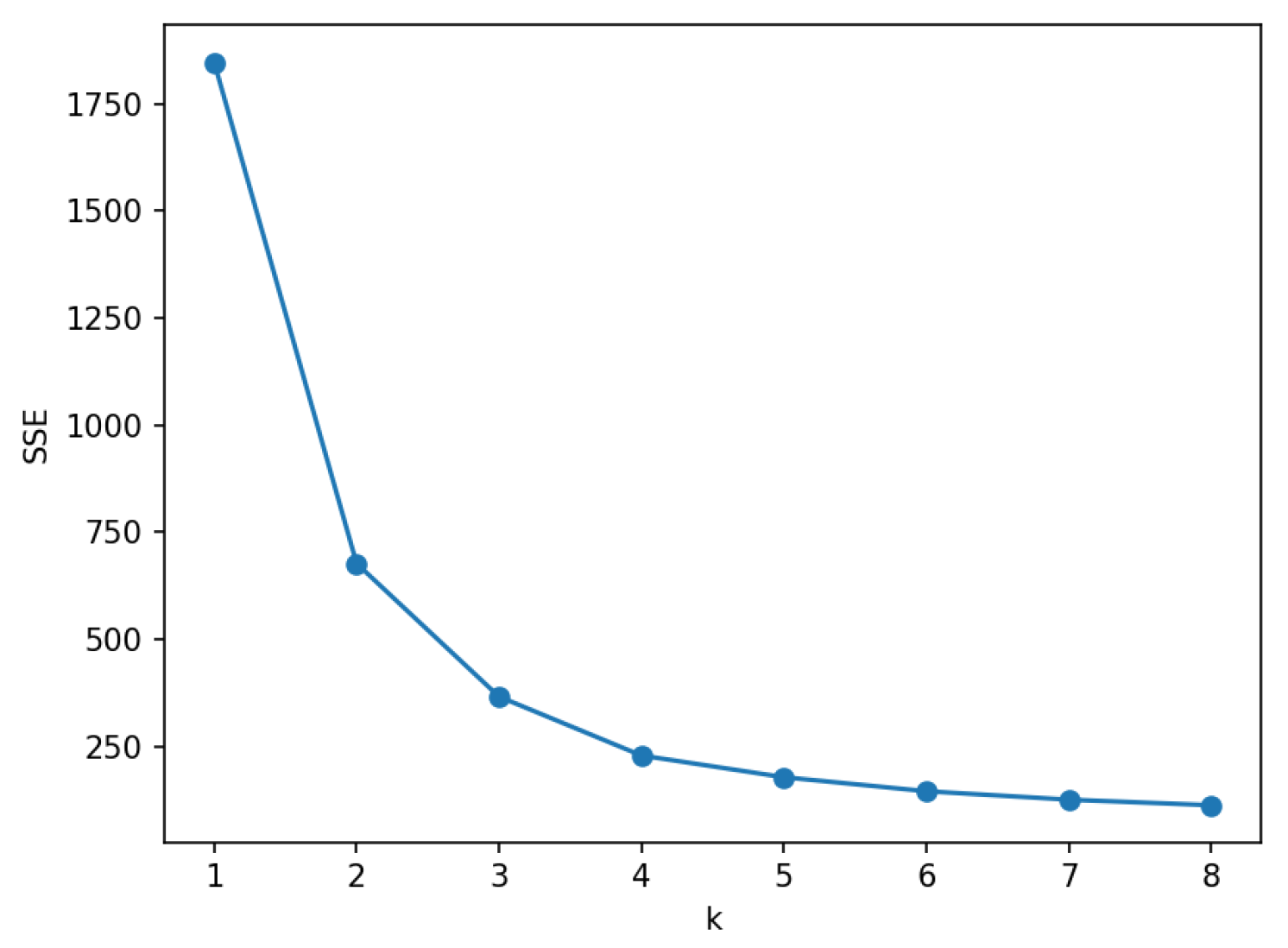
The choice of the k value in k-means significantly impacts condition classification accuracy. The elbow method helps determine the optimal k value as follows:

(a) Calculate the sum of squared errors (SSE) value:

Assume there are $\left\{n_1, n_2,\dots , n_k\right\}$ data samples in k clusters. The SSE is the sum of squared distances from each data point to its cluster center, calculated using Equation (5):

$$SSE=\sum _{j=1}^k\sum _{i=1}^n{‖x_{ij}-u_j‖}_2^2$$

(5)

(b) Plot SSE values against different k values.

(c) The SSE vs. k graph typically resembles an elbow, and the k value at the “elbow point” indicates the optimal cluster count for classification.

Three parameters (steam drum pressure, feedwater flow rate, and unit load) which are strongly correlated with the boiler operational state are used as sample co-ordinates for k-means classification. As shown in Figure 3, the k value corresponding to the elbow point is 2. Then, the experimental dataset is partitioned into two categories (condition 1 and condition 2), delineated by the boundaries of steam drum pressure, feedwater flow rate, and unit load. The parameter ranges for each type of operating condition, along with the quantity of data encompassed within each operational group, are itemized in Table 1, respectively.

Figure 3. SEE values at different k values.

Table 1. Parameter ranges of various operating conditions after classification.

Classification	Drum Pressure (MPa)	Feed Water Flow (t/h)	Unit Load (MW)	Data Volume
Condition 1	5.79–9.67	56.52–118.16	14.91–26.20	4634
Condition 2	8.22–10.18	83.88–152.94	24.16–32.25	16,917

2.2. Parameter Extraction

To improve model accuracy and reduce modeling time, tens of thousands of measurement points in the distributed control system (DCS) are screened. The average influence value method based on the BP neural network is used to screen the characteristic parameters of two output parameters, respectively:

(1)

Construct samples

Convert the initialization dataset into an independent variable matrix $\mathrm{X}={\left\{{\mathrm{X}}_1, {\mathrm{X}}_2, \dots , {\mathrm{X}}_{\mathrm{m}}\right\}}^{\mathrm{T}}$ with l rows and m columns and a dependent variable matrix $\mathrm{Y}={\left\{{\mathrm{Y}}_1, {\mathrm{Y}}_2, \dots , {\mathrm{Y}}_{\mathrm{m}}\right\}}^{\mathrm{T}}$ with m rows and 1 column, where l represents the number of data samples and m is the number of feature parameters.

(2)

Normalization processing

Normalized input parameters:

$$\begin{array}{c}\mathrm{x}\left(\mathrm{i},\mathrm{j}\right)=\frac{\mathrm{X}\left(\mathrm{i},\mathrm{j}\right)-{\mathrm{X}}_{\mathrm{m}\mathrm{i}\mathrm{n}}\left(\mathrm{i},\mathrm{j}\right)}{{\mathrm{X}}_{\mathrm{m}\mathrm{a}\mathrm{x}}\left(\mathrm{i},\mathrm{j}\right)-{\mathrm{X}}_{\mathrm{m}\mathrm{i}\mathrm{n}}\left(\mathrm{i},\mathrm{j}\right)}\end{array}$$

(6)

Normalized output parameters:

$$\begin{array}{c}\mathrm{y}\left(\mathrm{i}\right)=\frac{\mathrm{Y}\left(\mathrm{i}\right)-{\mathrm{Y}}_{\mathrm{m}\mathrm{i}\mathrm{n}}}{{\mathrm{Y}}_{\mathrm{m}\mathrm{a}\mathrm{x}}-{\mathrm{Y}}_{\mathrm{m}\mathrm{i}\mathrm{n}}}\end{array}$$

(7)

(3)

Establish a model

Using the normalized data from the previous step as input and output parameters, combined with the BP neural network algorithm, establish a prediction model for the target parameters.

(4)

Average impact value (AIV) analysis

Enlarge and shrink each column of the input parameter matrix to 1.1 and 0.9 times the original data to obtain the scaling matrices, as shown in Equations (8) and (9):

$$\begin{array}{c}{\mathrm{x}}_{\mathrm{j}}^1=\left[\begin{array}{c}{\mathrm{x}}_{11},{\mathrm{x}}_{12},\dots ,1.1{\mathrm{x}}_{1\mathrm{j}},\dots ,{\mathrm{x}}_{1\mathrm{n}}\\ {\mathrm{x}}_{21},{\mathrm{x}}_{22},\dots ,1.1{\mathrm{x}}_{2\mathrm{j}},\dots ,{\mathrm{x}}_{2\mathrm{n}}\\ ⋮\\ {\mathrm{x}}_{\mathrm{m}1},{\mathrm{x}}_{\mathrm{m}2},\dots ,1.1{\mathrm{x}}_{\mathrm{mj}},\dots ,{\mathrm{x}}_{\mathrm{mn}}\end{array}\right]\end{array}$$

(8)

$$\begin{array}{c}{\mathrm{x}}_{\mathrm{j}}^2=\left[\begin{array}{c}{\mathrm{x}}_{11},{\mathrm{x}}_{12},\dots ,0.9{\mathrm{x}}_{1\mathrm{j}},\dots ,{\mathrm{x}}_{1\mathrm{n}}\\ {\mathrm{x}}_{21},{\mathrm{x}}_{22},\dots ,0.9{\mathrm{x}}_{2\mathrm{j}},\dots ,{\mathrm{x}}_{2\mathrm{n}}\\ ⋮\\ {\mathrm{x}}_{\mathrm{m}1},{\mathrm{x}}_{\mathrm{m}2},\dots ,0.9{\mathrm{x}}_{\mathrm{mj}},\dots ,{\mathrm{x}}_{\mathrm{mn}}\end{array}\right]\end{array}$$

(9)

Place the scaled matrices $x_j^1$ and $x_j^2$ into the BP neural network model established in step (3) for prediction, and obtain the prediction results $y_j^1$ and $y_j^2$. The difference between two squares of $y_j^1$ and $y_j^2$ is calculated to obtain the influence value IV of the corresponding characteristic variable on the output parameter.

$$\begin{array}{c}\mathrm{I}{\mathrm{V}}_{\mathrm{j}}={\left(y_j^1\right)}^2-{\left(y_j^2\right)}^2\end{array}$$

(10)

(5)

Calculate the average of each IV value to obtain the AIV:

$$\begin{array}{c}\mathrm{A}\mathrm{I}{\mathrm{V}}_{\mathrm{j}}=\frac{1}{\mathrm{m}}{\displaystyle \sum _{i=1}^m}\mathrm{I}{\mathrm{V}}_{\mathrm{i}\mathrm{j}}\end{array}$$

(11)

(6)

Calculate contribution rate:

$${\mathsf{\eta }}_{\mathrm{j}}=\frac{\left|{\mathrm{A}\mathrm{I}\mathrm{V}}_{\mathrm{j}}\right|}{{\sum }_{\mathrm{i}=1}^{\mathrm{m}}\left|{\mathrm{A}\mathrm{I}\mathrm{V}}_{\mathrm{i}}\right|}$$

(12)

If the cumulative contribution rate of the set of feature variables reaches 80%, it is considered that there is a significant connection between the set of feature parameters and the output parameters, which are used as input parameters for the optimizing model.

2.3. Algorithm Optimization

In this study, the backpropagation neural network [9,15,16] with an input layer, a single hidden layer, and an output layer is selected as the core algorithm. The activation function for the hidden layer is set to sigmoid. At the same time, the random forest algorithm [17,18] is employed for comparison.

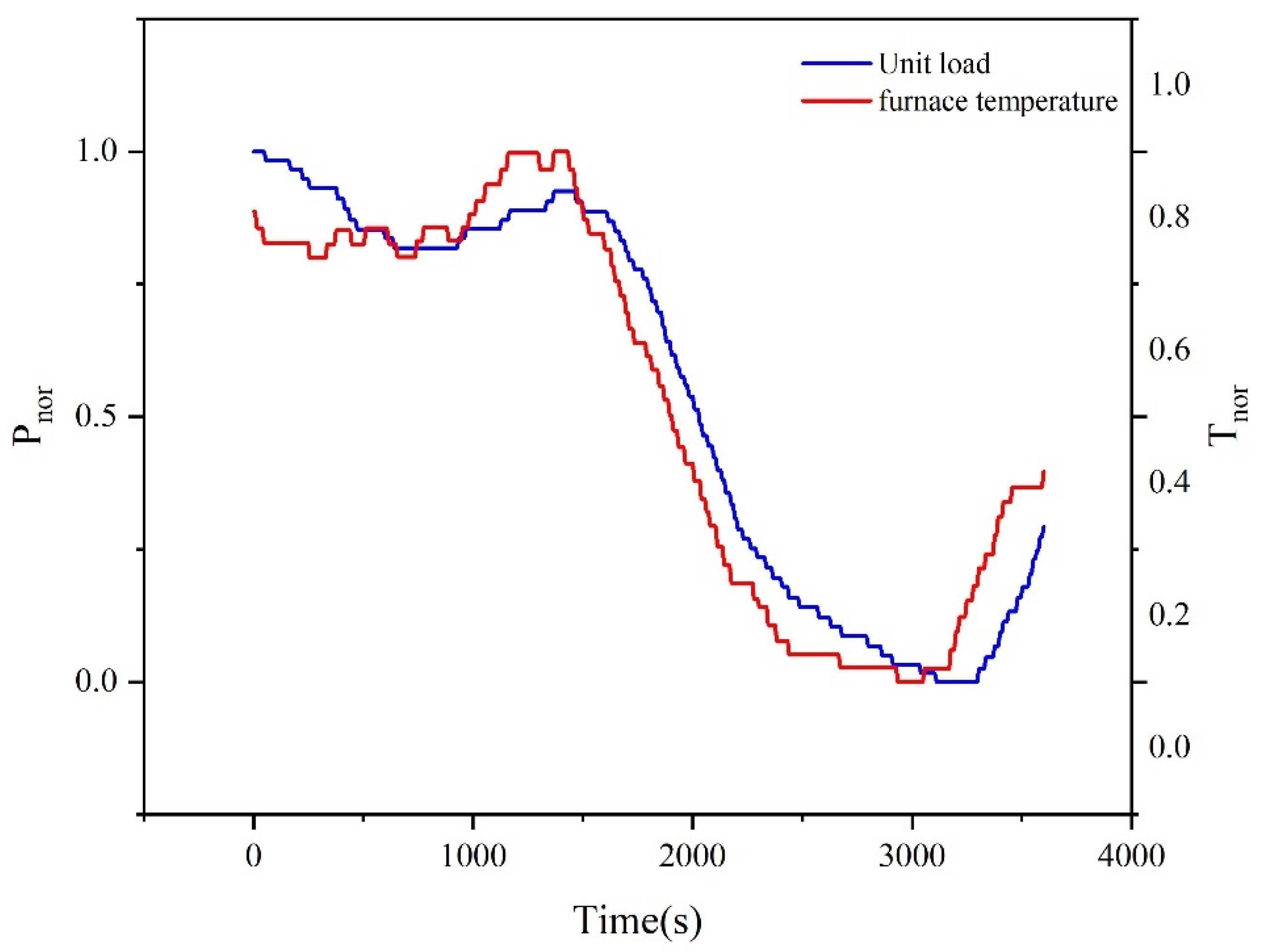
In practical applications, using only the BP algorithm poses challenges due to the asynchronous changes between input parameters, influenced by the control system and the inertia of combustion within the furnace, and the corresponding output parameters. The sampling process, indexed at the same time point, may compromise the model’s accuracy, especially when dealing with terminal output parameters like unit load in DCS systems, directly impacting the predictive model’s precision. Therefore, this study innovatively combines first-order derivative (FOD) with the BP algorithm. Additionally, a search mechanism based on ant colony optimization (ACO) is incorporated [19,20,21], enabling the FOD-BP-ACO model to effectively enhance boiler thermal efficiency.

Assume that the probability of ant k (k = 1, 2, …, m) transitioning from location i to location j at a certain moment is $p_{ij}^k$. The calculation formula is as follows:

$$p_{ij}^k=\left\{\begin{array}{c}\frac{{\tau }_{ij}^{\alpha } · {\eta }_{ij}^{\beta }}{{\sum }_{j-J_k\left(i\right)}{\tau }_{ij}^{\alpha } · {\eta }_{ij}^{\beta }},jϵ J_k\left(i\right)\\ 0, otherwise\end{array}\right.$$

(13)

In the equation, ${\tau }_{ij}^{\alpha }$ represents the amount of pheromone between location i and location j on the path at a certain moment, ${\eta }_{ij}^{\beta }$ represents the expected level of ant transitioning from i to j, $J_k\left(i\right)$ is the set of accessible locations for the ant in the next step, $\alpha$ is the importance factor of pheromone, and $\beta$ is the importance factor of heuristics. The operation of ant colony optimization is shown in Figure 4.

Figure 4. The operation of ant colony optimization.

When m ants complete one iteration of path traversal, typically, the ACO model is used to update the pheromone. The following formula can be used to update the pheromone concentration:

$${\tau }_{ij}\left(t+1\right)=\left(1-\rho \right)\cdot {\tau }_{ij}\left(t\right)+\mathsf{\Delta }{\tau }_{ij}\left(t\right)$$

(14)

In this formula, $\rho$ is the evaporation rate (a value between 0 and 1), and $\mathsf{\Delta }{\tau }_{ij}$ represents the amount of pheromone deposited by the ants on the path from i to j during the iteration.

This study does not aim to solve a path problem. Therefore, the two equations mentioned above will be rewritten to solve the maximization of a specified function:

$$\begin{array}{c}{p}_i=\frac{\underset{s\in \left[1,m\right]}{max}{\tau }_s\left(t\right)-{\tau }_i\left(t\right)}{\underset{s\in \left[1,m\right]}{max}{\tau }_s\left(t\right)}\end{array}$$

(15)

In this formula, ${\tau }_i\left(0\right)=F\left(X\right)$,${\tau }_0$ represents the initialization of pheromone values for the data. $F\left(X\right)$ represents the specified objective function and the optimization problem is transformed into a maximization problem; the formula for updating the pheromone concentration can be modified as follows:

$$\begin{array}{c}{\tau }_i\left(t+1\right)=\left(1-\rho \right){\tau }_i\left(t\right)+Q\times F\left(X\right)\end{array}$$

(16)

$Q$ represents the total pheromone concentration released by the ants after completing one iteration or cycle. As $F\left(X\right)$ increases, it indicates a higher value of the objective function, which, in turn, leads to a larger overall pheromone concentration at the location where the ants are located.

The introduction of the ACO algorithm significantly enhances the local search capability of the BP algorithm. Additionally, to improve the precision of the predictive model, this study proposes the optimization of BP through the introduction of FOD. The FOD is used to estimate the delay time of a particular parameter relative to another output parameter within a given system or process, and the specific process is as follows:

Firstly, calculate the Pearson correlation coefficient of the unit load characteristic parameters with Equation (17):

$$\mathrm{r}=\frac{{\sum }_{\mathrm{i}=1}^{\mathrm{n}}\left({\mathrm{X}}_{\mathrm{I}}-\overline{\mathrm{X}}\right)\left({\mathrm{Y}}_{\mathrm{i}}-\overline{\mathrm{Y}}\right)}{\sqrt{{\sum }_{\mathrm{i}=1}^{\mathrm{n}}{\left({\mathrm{X}}_{\mathrm{I}}-\overline{\mathrm{X}}\right)}^2}\sqrt{{\sum }_{\mathrm{i}=1}^{\mathrm{n}}{\left({\mathrm{Y}}_{\mathrm{i}}-\overline{\mathrm{Y}}\right)}^2}}$$

(17)

Next, conduct a lag analysis by selecting representative parameters with a correlation coefficient greater than 0.5 relative to the unit load from the input parameters. Subsequently, the interpolation function is fitted to the scattered data points over a complete period, the FOD of the fitted function is performed, and the estimation of the parameter relative to the output parameter is obtained by comparing the time difference between adjacent extreme points delay.

Assuming there are n hysteresis-compensated operating state parameters, for $i=\left\{1,2\dots n\right\}$, define the latency $t_{di}$ as shown in the following Equation (18):

$$\left\{\begin{array}{c}\begin{array}{c}{\mathrm{P}}^{\prime }\left({\mathrm{t}}_{\mathrm{p}}\right)=0\\ {\mathrm{P}}^{\prime }\left({\mathrm{t}}_{\mathrm{p}}-{\mathrm{t}}_{\mathrm{s}}\right){\mathrm{P}}^{\prime }\left({\mathrm{t}}_{\mathrm{p}}+{\mathrm{t}}_{\mathrm{s}}\right)<0\end{array}\\ \begin{array}{c}{\mathrm{B}}_{\mathrm{i}}^{\prime }\left({\mathrm{t}}_{\mathrm{b}}\right)=0\\ {\mathrm{B}}_{\mathrm{i}}^{\prime }\left({\mathrm{t}}_{\mathrm{b}\mathrm{i}}-{\mathrm{t}}_{\mathrm{s}}\right){\mathrm{B}}_{\mathrm{i}}^{\prime }\left({\mathrm{t}}_{\mathrm{b}\mathrm{i}}+{\mathrm{t}}_{\mathrm{s}}\right)<0\end{array}\\ \begin{array}{c}0<{\mathrm{t}}_{\mathrm{b}\mathrm{i}}-{\mathrm{t}}_{\mathrm{p}}<{\mathrm{t}}_{\mathrm{d}\mathrm{m}\mathrm{a}\mathrm{x}}\\ {\mathrm{t}}_{\mathrm{d}\mathrm{i}}={\mathrm{t}}_{\mathrm{b}}-{\mathrm{t}}_{\mathrm{p}}\end{array}\end{array}\right.$$

(18)

where $P$ is for unit load, $B_i$ is the ith hysteresis-compensated operating state parameter, $t_p$ is for the unit load interpolation function corresponding to the extreme value point, $t_b$ represents the ith running parameter interpolating the extremum point corresponding to the time, $t_s$ represents DCS sampling interval, $t_{di}$ represents the latency for running parameter $B_i$, and ${ t}_{dmax}$ is for maximum lag time of biomass boiler unit load.

The FOD-BP algorithm corrects the weights and thresholds of hidden layer nodes by propagating the error values generated after forward propagation back to the hidden layer, distributing them across the nodes. This process is iteratively repeated until the iteration reaches the minimum error value and concludes.

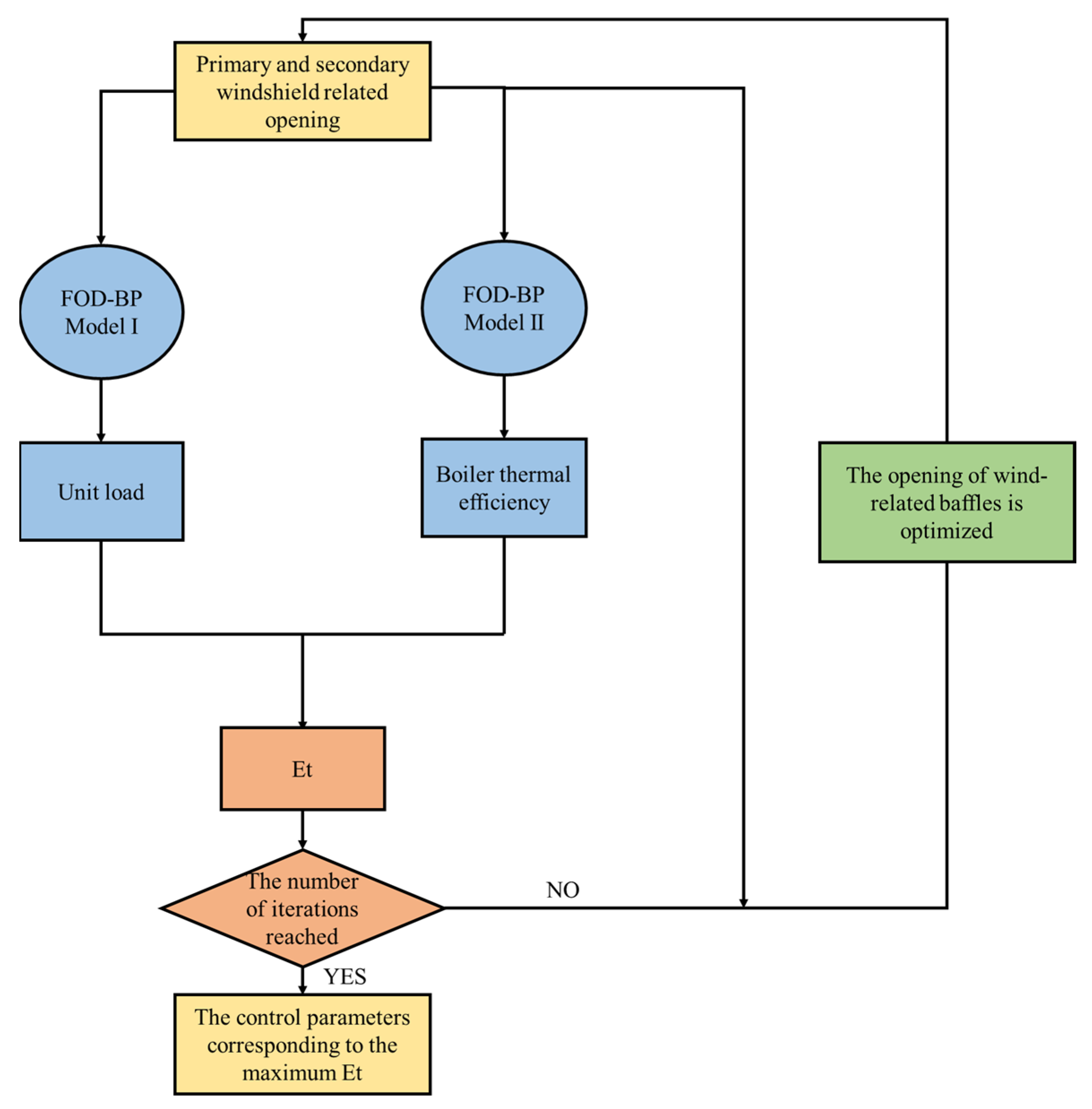
The FOD-BP model is a hybrid neural network based on the traditional BP algorithm. To enhance the local search capability of the BP algorithm, the ACO algorithm is introduced into the network’s weight-updating mechanism. The FOD algorithm adjusts the delay time difference to provide accurate input parameters for the BP algorithm, improving the model accuracy. By combining the FOD and ACO algorithms, it effectively obtains more accurate input parameters, thereby enhancing the precision of the BP model and maximizing thermal efficiency through control parameter adjustments.

3. Results and Discussion

3.1. FOD Compensation Result

As shown in Figure 5, there exists a certain linear correlation between the unit load and furnace temperature. Moreover, it is observable that, when the time changes, the load changes exhibit a noticeable lag compared to the furnace temperature curve. Therefore, we introduce the first derivative method to improve the model accuracy.

Figure 5. Unit load–furnace temperature variation.

Thus, parameters whose Pearson correlation coefficients are greater than 0.50 with the unit load are selected as compensation parameters in Table 2.

Table 2. Hysteresis analysis parameters.

Parameter Name	Unit	Correlation Coefficient
Feed water flow	t/h	0.95
Feed water pump pressure	MPa	0.94
Drum pressure	MPa	0.94
Furnace temperature	°C	0.52

The average lag time for each compensation parameter is shown in Table 3. The compensation effect is verified using data from unit load operating condition 2, 70% of the data are randomly selected as the training set, 30% of the data are used as the test set, and the model prediction results before and after compensation are shown in Figure 6. The mean relative error (MRE) is reduced by 15.64% after hysteresis compensation compared to before hysteresis (as shown in Table 4). This indicates that FOD compensation can improve forecasting accuracy to a certain extent.

Table 3. Lag time for compensation parameter.

Parameter Name	Compensation Time (s)
Feed water flow	8 s
Feed pump outlet pressure	40 s
Drum pressure	40 s
Furnace temperature	56 s

Figure 6. Compensation effect: (a) compensation before unit load forecast results; and (b) unit load forecast results after compensation.

Table 4. Performance evaluation parameters of boiler thermal efficiency prediction model before and after compensation.

Type of Data	MAE (MW)	MRE (%)	RMSE (MW)	R2
Before compensation	0.1992	0.69	0.2322	0.9788
After compensation	0.1683	0.58	0.2195	0.9811

Note: mean absolute error—MAE.

3.2. Unit Load and Boiler Efficiency Prediction

Predictive models for the unit load and boiler thermal efficiency under two different operating conditions were established using the random forest algorithm and the BP neural network algorithm, and a comparison of the predictive results between the two algorithms was conducted.

3.2.1. Random Forest Model

We used grid-search–cross-validation-optimized hyperparameters for unit load forecasting using a dataset of operating condition 2, with R² as the evaluation index. Similar tuning was applied to other datasets, yielding optimal points as detailed in Table 5.

Table 5. Optimization results of random forest hyperparameters.

Parameter Name	Unit Load		Boiler Thermal Efficiency
	Condition 1	Condition 2	Condition 1	Condition 2
T	80	70	80	70
Max depth	8	8	6	7

It can be observed from Table 6 that, apart from the unit load condition 1, the relative errors of the random forest predictive models for all operating conditions are below 1%, with R² values exceeding 0.95. Among them, the single model with the highest accuracy is the boiler thermal efficiency predictive model 1, which has an average MRE of only 0.02%.

Table 6. Evaluation metrics for random forest prediction models.

Evaluation Index	Unit Load		Boiler Thermal Efficiency
	Condition 1	Condition 2	Condition 1	Condition 2
MAE	0.2422	0.2076	0.0208	0.0690
MRE (%)	1.10	0.72	0.02	0.08
RMSE	0.3653	0.2929	0.0452	0.1061
R2	0.9854	0.9664	0.9997	0.9980

3.2.2. BP Neural Network

BP neural network models were developed using the PyCharm Community edition 2023.2. The model parameters settings are presented in Table 7.

Table 7. Parameter settings for the BP neural network prediction model.

Parameter	Number
Maximum iteration steps	1000
Learning rate	0.001
Batch size	16

Taking the unit load as an example, the number of input layer nodes was 38, and the range of hidden layer nodes given according to different empirical formulae is l < 60, with comprehensive consideration, and 11 numbers in the range of 5–55 were taken at intervals of 5. Similarly, the hidden layer node selection was carried out for the thermal efficiency of the boiler, and the BP neural network prediction model was established by using the data after the division of operating conditions, and the root mean square error (RMSE) corresponding to the number of nodes is shown in Table 8.

Table 8. The number of hidden layer nodes of operating condition 1 predictive model corresponds to the RMSE.

The Number of Hidden Layer Nodes	Unit Load RMSE	The Number of Hidden Layer Nodes	Boiler Thermal Efficiency RMSE
5	0.3837	5	0.0651
10	0.3413	8	0.0760
15	0.3202	10	0.1127
20	0.2870	13	0.0416
25	0.2720	15	0.0385
30	0.2714	18	0.1171
35	0.2648	20	0.0382
40	0.2486	25	0.0255
45	0.2655	30	0.0195
50	0.2568	35	0.0223
55	0.2858	40	0.0163

The number of nodes corresponding to the lowest RMSE of the above two types of operating conditions is shown in Table 9.

Table 9. The optimal number of hidden layer nodes in a BP neural network.

Evaluation Index	Unit Load		Boiler Thermal Efficiency
	Condition 1	Condition 2	Condition 1	Condition 1
The number of hidden layer nodes	40	45	40	23

The results of BP neural network predictions are shown in Figure 7.

Figure 7. Results of BP neural network: (a) prediction results of thermal efficiency of boilers under condition 1; (b) prediction results of thermal efficiency of boilers under condition 2; (c) prediction results of unit load under condition 1; and (d) prediction results of unit load under condition 2.

From Table 10, it can be seen that the mean relative error of the BP neural network predictive model under all operating conditions is within 1.5%, and the value of R² is above 0.94, among which the single model with the highest accuracy is the boiler thermal efficiency prediction model under operating conditions 1, and its mean relative error is only 0.04%. In summary, the BP neural network prediction model can accurately predict the boiler thermal efficiency and unit load under all operating conditions.

Table 10. Evaluation metrics for BP neural network prediction models.

Evaluation Index	Unit Load		Boiler Thermal Efficiency
	Condition 1	Condition 2	Condition 1	Condition 2
MAE	0.1882	0.1671	0.0118	0.0169
MRE (%)	0.88	0.58	0.01	0.02
RMSE	0.2486	0.2157	0.0163	0.0222
R2	0.9932	0.9818	0.9995	0.9991

A detailed comparison is as follows:

(1)

Unit load: For condition 1, the MRE of the random forest predictive model is 1.10%, while the MRE of the BP neural network predictive model is 0.88%. This represents a decrease of approximately 25% in the MRE compared to the random forest predictive results. For condition 2, the random forest predictive model has an MRE of 0.72%, while the BP neural network predictive model has an MRE of 0.58%. In this case, the MRE of the BP neural network predictive model is approximately 24.1% lower than that of the random forest.

(2)

Thermal efficiency: For condition 1, the MRE value of the BP neural network predictive model decreased by approximately 100% compared to the random forest predictive results. For condition 2, the decrease was approximately 300%.

The BP neural network algorithm maintains an MRE of within 1.5% in all predictive models, indicating an overall superior predictive performance compared to random forest. Taking into account both modeling accuracy and stability, the next section will proceed with the optimization of control parameters using the model established by the BP neural network algorithm.

3.3. Optimization of Boiler Efficiency Using Ant Colony Algorithm

One-hour datasets were randomly selected for each type of operating condition and the ant colony algorithm was used to search for the corresponding damper positions that maximize boiler efficiency. The hyperparameters of the ant colony algorithm are shown in Table 11, and the variation range of the independent variable (high-side, center, and low-side boiler grate air damper positions, as well as front and rear furnace wall secondary air damper positions) of the objective function was specified to be 0.9–1.1 times of the original value and the opening of the baffle was not higher than 100%. The FOD-BP neural network models obtained were selected for the forward prediction model. The changes of the high-side, center-side, and low-side exhaust air damper opening, the secondary air damper opening of the front wall and the rear wall of the furnace, and boiler efficiency, before and after optimization, are shown in Table 11. The FOD-BP forecast value is the value obtained from the initial input parameters, and the FOD-BP-ACO forecast value is the value obtained from the input parameters after optimization.

Table 11. Hyperparameter configuration for BP ant colony algorithm.

Parameter	Number
Iterations	100
Ant population	100
Information evaporation coefficient	0.8
Cumulative information release	1

The results show that the thermal efficiency of the boiler increases by 0.002–0.04% compared with the pre-optimization value. However, it is worth noting that, in certain instances, such as at 2160 s, even with optimization, the thermal efficiency remains below the actual values, albeit with a 0.02% improvement. This is primarily due to the initial predictive model having some degree of error, resulting in significant deviations between the predicted and actual values, even after optimization. Out of the 902 datasets analyzed, 95% of them demonstrated an improvement in boiler thermal efficiency by 0.01–0.06% relative to the actual values when the unit load variation did not exceed 0.5 MW. The performance data for different parameter types is summarized in Table 12.

Table 12. Performance data for different parameter types.

Time(s)	Parameter Type	Front Wall Secondary Air Damper Opening (%)	Rear Wall Secondary Air Damper Opening (%)	High-Side Boiler Grate Air Damper Opening (%)	Center Boiler Grate Air Damper Opening (%)	Low-side Boiler Grate Air Damper Opening (%)	Unit Load (MW)	Efficiency (%)	E* − E (True)	E (FOD-BP-ACO) − E (FOD-BP)
240	True value	100.00	100.00	54.91	25.98	26.34	31.860	86.602
	FOD-BP	100.00	100.00	54.91	25.98	26.34	31.928	86.625	0.022
	FOD-BP-ACO	97.30	92.25	56.43	24.92	25.41	31.955	86.638	0.036	0.013
480	True value	40.87	40.32	35.47	36.29	36.29	31.880	86.601
	FOD-BP	40.87	40.32	35.47	36.29	36.29	31.626	86.600	-0.001
	FOD-BP-ACO	42.47	41.91	34.31	34.91	33.90	31.674	86.614	0.012	0.013
720	True value	50.09	63.71	45.63	31.11	26.01	31.310	86.604
	FOD-BP	50.09	63.71	45.63	31.11	26.01	31.590	86.634	0.030
	FOD-BP-ACO	48.29	69.45	43.45	29.63	24.48	31.581	86.641	0.037	0.007
960	True value	72.31	76.40	54.95	26.43	26.31	30.750	86.606
	FOD-BP	72.31	76.40	54.95	26.43	26.31	30.908	86.641	0.035
	FOD-BP-ACO	67.89	82.51	53.59	24.89	24.81	30.901	86.647	0.041	0.006
1200	True value	76.43	76.53	54.82	26.37	26.37	30.470	86.678
	FOD-BP	76.43	76.53	54.82	26.37	26.37	30.590	86.709	0.031
	FOD-BP-ACO	70.81	82.11	53.95	25.04	24.80	30.589	86.715	0.037	0.006
1440	True value	76.34	76.74	54.85	27.59	26.31	30.480	86.679
	FOD-BP	76.34	76.74	54.85	27.59	26.31	30.378	86.706	0.028
	FOD-BP-ACO	73.76	83.78	54.15	26.30	25.97	30.339	86.711	0.033	0.005
1680	True value	76.83	76.37	54.95	26.01	26.37	31.610	86.678
	FOD-BP	76.83	76.37	54.95	26.01	26.37	31.414	86.711	0.034
	FOD-BP-ACO	78.33	81.39	55.73	24.65	24.97	31.415	86.716	0.038	0.005
1920	True value	100.00	99.91	55.25	26.28	25.98	30.670	86.606
	FOD-BP	100.00	99.91	55.25	26.28	25.98	30.399	86.625	0.019
	FOD-BP-ACO	93.20	91.11	56.87	24.87	25.60	30.526	86.639	0.034	0.014
2160	True value	98.26	98.84	52.47	36.36	36.36	30.37	86.605
	FOD-BP	98.26	98.84	52.47	36.36	36.36	30.418	86.568	−0.037
	FOD-BP-ACO	100.00	89.70	54.01	33.83	34.85	30.459	86.592	−0.012	0.024
2400	True value	59.92	71.31	32.39	32.97	26.40	29.200	86.607
	FOD-BP	59.92	71.31	32.39	32.97	26.40	28.983	86.617	0.010
	FOD-BP-ACO	55.79	64.99	33.16	31.35	25.01	29.107	86.629	0.022	0.012
2640	True value	88.58	100.00	54.88	26.65	26.31	30.060	86.534
	FOD-BP	88.58	100.00	54.88	26.65	26.31	30.107	86.558	0.024
	FOD-BP-ACO	82.27	94.39	54.45	25.19	25.06	30.166	86.569	0.035	0.011
2880	True value	100.00	100.00	54.88	27.50	25.98	30.930	86.534
	FOD-BP	100.00	100.00	54.88	27.50	25.98	30.896	86.550	0.016
	FOD-BP-ACO	92.67	94.45	57.76	26.83	25.66	31.006	86.564	0.031	0.014
3120	True value	100.00	100.00	54.98	27.47	25.98	31.200	86.534
	FOD-BP	100.00	100.00	54.98	27.47	25.98	31.262	86.551	0.017
	FOD-BP-ACO	94.29	92.57	56.85	26.39	25.88	31.360	86.566	0.032	0.015

Note that E* represents the efficiency of this column.

4. Conclusions

In this paper, a prediction model based on FOD-BP-ACO is proposed to optimize the controlling parameter of the biomass boiler. The main conclusions are summarized below:

The k-means clustering method is introduced to categorize data into two distinct operational states based on boundary parameters (steam drum pressure, feedwater flow rate, and unit load). When the delay parameter compensation is used, the average relative error of the model is reduced by 25.78%, which indicates that the delay compensation can effectively improve the accuracy of the prediction. The ant colony algorithm is proposed to optimize the air damper opening and show that the thermal efficiency of the boiler increases by 0.002–0.04% (relative to the predicted value) and 95% of the data demonstrated an improvement in boiler thermal efficiency by 0.01–0.06% relative to the actual values. This improvement is limited, because the model was based on the data of optimized operation condition and fixed biomass fuel. When the type of biomass fuel varies in a large range, FOD-BP-ACO might show a good potential for boiler efficiency improvement and providing a new reference for establishing the intelligent control system of biomass boilers.

References

1. International Renewable Energy Agency. Renewable Capacity Statistics 2023. Available online: https://www.irena.org/Publications/2023/Mar/Renewable-capacity-statistics-2023 (accessed on 26 March 2023).
2. Li, G.; Niu, P.; Wang, H.; Liu, Y. Least Square Fast Learning Network for modeling the combustion efficiency of a 300WM coal-fired boiler. Neural Netw. 2014, 51, 57–66. [Google Scholar] [CrossRef] [PubMed]
3. Krzywanski, J.; Czakiert, T.; Blaszczuk, A.; Rajczyk, R.; Muskala, W.; Nowak, W. A generalized model of SO2 emissions from large- and small-scale CFB boilers by artificial neural network approach: Part 1. The mathematical model of SO2 emissions in air-firing, oxygen-enriched and oxycombustion CFB conditions. Fuel Process. Technol. 2015, 137, 66–74. [Google Scholar] [CrossRef]
4. Krzywanski, J.; Czakiert, T.; Blaszczuk, A.; Rajczyk, R.; Muskala, W.; Nowak, W. A generalized model of SO2 emissions from large- and small-scale CFB boilers by artificial neural network approach Part 2. SO2 emissions from large- and pilot-scale CFB boilers in O2/N2, O2/CO2 and O2/RFG combustion atmospheres. Fuel Process. Technol. 2015, 139, 73–85. [Google Scholar] [CrossRef]
5. Gao, X.; Fu, Z.; Zhang, L.; Liu, B. Research on the Application of Big Data Technology in the Development of Coal-Fired Power Plants. J. Shenyang Inst. Eng. 2018, 14, 16–22. [Google Scholar]
6. Li, Y.Y. Research on the Prediction and Control System of Nitrogen Oxides Emissions from Power Plant Boilers. Ph.D. Dissertation, Northeast Electric Power University, Jilin, China, 2020. [Google Scholar]
7. Blackburn, L.D.; Tuttle, J.F.; Andersson, K.; Hedengren, J.D.; Powell, K.M. Dynamic machine learning-based optimization algorithm to improve boiler efficiency. J. Process Control. 2022, 120, 129–149. [Google Scholar] [CrossRef]
8. Yao, Z.; Romero, C.; Baltrusaitis, J. Combustion optimization of a coal-fired power plant boiler using artificial intelligence neural networks. Fuel 2023, 344, 128145. [Google Scholar] [CrossRef]
9. Tian, W.; Cao, Y. Evaluation model and algorithm optimization of intelligent manufacturing system on the basis of BP neural network. Intell. Syst. Appl. 2023, 20, 200293. [Google Scholar] [CrossRef]
10. Maharana, K.; Mondal, S.; Nemade, B. A review: Data pre-processing and data augmentation techniques. Glob. Transit. Proc. 2022, 3, 91–99. [Google Scholar] [CrossRef]
11. Xia, J.; Zhang, J.; Wang, Y.; Han, L.; Yan, H. WC-KNNG-PC: Watershed clustering based on k-nearest-neighbor graph and Pauta Criterion. Pattern Recognit. 2022, 121, 108177. [Google Scholar] [CrossRef]
12. Ay, M.; Özbakır, L.; Kulluk, S.; Gülmez, B.; Öztürk, G.; Özer, S. FC-Kmeans: Fixed-centered K-means algorithm. Expert Syst. Appl. 2023, 211, 118656. [Google Scholar] [CrossRef]
13. Selim, S.Z.; Ismail, M.A. K-means-type algorithms: A generalized convergence theorem and characterization of local optimality. IEEE Trans. Pattern Anal. Mach. Intell. 1984, 6, 81–87. [Google Scholar] [CrossRef] [PubMed]
14. Liu, B.; Fu, Z.; Wang, P.; Liu, L.; Gao, M.; Liu, J. Big-Data-Mining-Based Improved K-Means Algorithm for Energy Use Analysis of Coal-Fired Power Plant Units: A Case Study. Entropy 2018, 20, 702. [Google Scholar] [CrossRef] [PubMed]
15. Wang, J.; Zou, B.; Liu, M.; Li, Y.; Ding, H.; Xue, K. Milling force prediction model based on transfer learning neural network. J. Intell. Manuf. 2020, 32, 947–956. [Google Scholar] [CrossRef]
16. Huang, X.; Li, Q.; Tai, Y.; Chen, Z.; Zhang, J.; Shi, J.; Cao, B.; Liu, W. Hybrid deep neural model for hourly solar irradiance forecasting. Renew. Energy 2021, 171, 1041–1060. [Google Scholar] [CrossRef]
17. Gall, J.; Lempitsky, V. Class-specific Hough forests for object detection. In Proceedings of the 2009 IEEE Conference on Computer Vision and Pattern Recognition, Miami, FL, USA, 20–25 June 2009. [Google Scholar]
18. Breiman, L. Random Forests. Mach. Learn. 2001, 45, 5–32. [Google Scholar] [CrossRef]
19. Cui, J.; Guo, X.; Zhan, Y.; Pang, R. An inverse analysis method to identify maximum overfire temperature based on an improved ant colony algorithm. J. Build. Eng. 2022, 59, 105104. [Google Scholar] [CrossRef]
20. Dorigo, M.; Gambardella, L.M. Ant Colony System: A cooperative learning approach to the traveling salesman problem. IEEE Trans. Evol. Comput. 1997, 1, 53–66. [Google Scholar] [CrossRef]
21. Mirjalili, S.; Mirjalili, S.S.; Lewis, A. Grey Wolf Optimizer. Adv. Eng. Softw. 2014, 69, 46–61. [Google Scholar] [CrossRef]
Disclaimer/Publisher’s Note: The statements, opinions and data contained in all publications are solely those of the individual author(s) and contributor(s) and not of MDPI and/or the editor(s). MDPI and/or the editor(s) disclaim responsibility for any injury to people or property resulting from any ideas, methods, instructions or products referred to in the content.
Article Metrics
Citations
Article Access Statistics
Multiple requests from the same IP address are counted as one view.