Optimum Design of a Reusable Spacecraft Launch System Using Electromagnetic Energy: An Artificial Intelligence GSO Algorithm

Abstract

Due to its advantages of high acceleration, reusability, environmental protection, safety, energy conservation, and efficiency, electromagnetic energy has been considered as an inevitable choice for future space launch technology. This paper proposes a novel three-level orbital launch approach based on a combination of a traditional two-level orbital launch method and an electromagnetic boost (EMB), in which the traditional two-level orbital launch consists of a turbine-based combined cycle (TBCC) and a reusable rocket (RR). Firstly, a mathematical model of a multi-stage coil electromagnetic boost system is established to develop the proposed three-level EMB-TBCC-RR orbital launch approach, achieving a horizontal take-off–horizontal landing (HTHL) reusable launch. In order to optimize the fuel quality of the energy system, an artificial intelligence algorithm parameters-sensitivity-based adaptive quantum-inspired glowworm swarm optimization (AQGSO)is proposed to improve the performance of the electromagnetic boosting system. Simulation results show that the proposed AQGSO improves the global optimization precision and convergence speed. By using the proposed EMB-TBCC-RR orbital launch system and the optimization approach, the required fuel weight was reduced by about 13 tons for the same launch mission, and the energy efficiency and reusability of the spacecraft was greatly improved. The spacecraft can be launched with more cargo capacity and increased payload. The proposed novel three-level orbital launch approach can help engineers to design and optimize the orbital launch system in the field of electromagnetic energy conversion and management.

1. Introduction

Various approaches to space launching have experienced rapid development over the last few decades [1,2]. Nevertheless, traditional disposable chemical energy rockets are still commonly used in space launch missions. Thus, the development of energy-efficient space launch approaches remains a research hotspot in the field of aviation and aerospace. Currently, several disadvantages of traditional chemical energy rocket technology are yet to be overcome: (1) chemical energy rocket technology has approached its theoretical mass limit for launch missions, but several marginal effects can be improved [3]; (2) air pollution is associated with the combustion process; (3) the ratio of the payload to the total take-off weight of a launch vehicle is very low in chemical energy rockets, i.e., a few percent for low earth orbit (LEO), and as low as one percent for geosynchronous orbit (GTO). This means that the launch cost is very expensive in regards to a conventional chemical energy launch mission. The unit kg payload delivery cost of Falcon 9 can be reduced from approximately 20000 USD to 800 USD through reusable design [4]. (from USD 4000 to USD 20,000 per kilo) [4].

Therefore, the energy-efficient launch approach has become a research hotspot, with the goal of improving energy efficiency and thus reducing the launch cost. Many advanced launch technologies have been researched [5,6,7,8,9,10,11,12,13], such as the multidisciplinary design approach [5], the use of a space elevator [6], reusable launch vehicles [7,8], and an electromagnetic boost launch system [9,10,11]. Using these technologies, reusable vehicles and electromagnetic boost launch system are proven to have high feasibility and efficiency.

Currently, the technology regarding a reusable launch consists of employing the aspirated two-stage to orbit (TSTO) approach, which uses oxygen in the atmosphere as the fuel in order to reduce the take-off weight and technical risks, as well as to ensure the ease of implementation, thus improving the launch economy and efficiency. As a durable reusable carrier, the space shuttle is partially re-used for the launch mission, i.e., the rocket-launched aircraft X-37B and the X43A powered by a scramjet engine. It is worth mentioning that the success of reusable launch technology from SpaceX indicates that reusable launch technology will continue to develop rapidly. Moreover, Russia, Europe, India, Japan, and China have paid increasing attention to the development of reusable launch technology, as can be seen in the Russian Clipper, the European Space Agency FLTP plan, the Britain Skylon, etc.

Different from the conventional mechanical or chemical launch mode, electromagnetic space launch systems (EMSLs) use electromagnetic propulsion to achieve acceleration at high- or ultra-high-speeds. They exhibit great advantages over chemical energy launched rockets, i.e., EMSLs can launch rockets with a larger useful load and a higher acceleration, reusability, energy conservation, efficiency, environmental protection, and safety. EMSLs have been developed with applications for various space launch modes from ground-based launches [10], airborne launches [11], the electromagnetic acceleration of superconductors [12], and the augmentation of a permanent magnet linear synchronous motor [13]. In 2018, McNab evaluated a two-stage-to-low-Earth-orbit projectile for space launches. The initial velocity is provided by EMSLs [13]. An optimized design of an EM coil gun system is created for a GEO launch task, in which the energy costs of the electromagnetic launching system are minimized [14]. Multi-pole field electromagnetic launching is a novel electromagnetic launching technology. It improves the performance of some techniques of traditional inductive electromagnetic emission technology. This type electromagnetic launching technology is suitable for high quality, large caliber projectiles with a high-speed launch potential [15]. This advanced approach EMSLs can be considered as an inevitable method for future launch technology.

This paper proposes a novel three-level orbital launch approach based on a combination of a reusable two-level orbital launch method and an electromagnetic boost (EMB) system in which the reusable two-level orbital launch consists of a turbine-based combined cycle (TBCC) and a reusable rocket (RR). The proposed approach uses electromagnetic boosting to achieve a horizontal take-off–horizontal landing (HTHL) reusable launch.

Electromagnetic effects are impacted by many factors, such as magnet material, magnet shape, configuration, quantity, spacing, number of coils, coil size, length, etc. [16]. Therefore, the electromagnetic effect is nonlinearly strong and multivariable. The optimization design for the electromagnetic effects is very complicated [17]. When studying the energy harvester based on the electromagnetic effect, the literature [18] develops an electromagnetic energy harvesting device based on a sprung eccentric rotor, and the optimization and characterized analysis of the electromagnetic system are presented. In Ref. [19], an electromagnetic thermal-fluid kinetic model is proposed for microwave-assisted production, and the simulated model included the effects of electromagnetic propagation. From the previous electromagnetic energy applications, the electromagnetic energy can be reasonably considered as an inevitable method for future space launch technology due to its advantages including high acceleration, reusability, environmental protection, safety, energy savings, and efficiency.

The scheduled launch mission can be completed using less fuel through the use of electromagnetic acceleration. This paper establishes a mass estimation model for the proposed three-stage launch system. The model takes the parameters of the electromagnetic launch system as input, and the take-off weight of the reusable vehicle is considered as output. To minimize the take-off weight of a reusable vehicle, we use an optimization algorithm to optimize the design scheme of the proposed three-stage-to-orbit launch approach for the purpose of reducing the vehicle’s launch weight.

Over the last few years, a number of new swarm intelligence algorithms have been proposed. A very interesting new population-based swarm intelligence algorithm that simulates the movement of the glowworms in a swarm based on the distance between them and on a luminescent quantity called luciferin is called the glowworm swarm optimization(GSO) algorithm, presented by Krishnanand and Ghose [20,21].The algorithm shares a few features with some better known swarm intelligence-based optimization algorithms, such as colony optimization and particle swarm optimization, but with several significant differences. The performance of the GSO regarding various benchmark multimodal functions, which have multiple local optima, is analyzed, and the results prove that the GSO outperforms PSO [22,23].

Therefore, this paper firstly uses the standard GSO (SGSO) algorithm to optimize the electromagnetic boost portions of the three-stage-to-orbit system. But due to the inherent defects of the GSO algorithm, the optimization effect of the three-stage-to-orbit system is not satisfactory. Therefore, a novel adaptive quantum GSO (AQGSO) algorithm is designed by integrating quantum computing, genetic mutation, and sensitivity analysis. The superiority of the AQGSO algorithm is verified by comparison of the optimization results with those of the other two algorithms, and the optimal design scheme is obtained. This paper is organized as follows: the schematic of this paper is introduced in Section 2. The overall concept of the proposed electromagnetic boost HTHL launch approach is presented in Section 3. Section 4 analyses the parameter sensitivity of the electromagnetic boost portion of the three-stage-to-orbit launch approach. Section 5 presents the adaptive quantum GSO algorithm. Section 6 carries out the launch system energy optimization using different optimization algorithms and analyzes the design results.

2. The Motivation for the Proposed Launch Approach

As shown in this Figure 1, the motivation for the proposed launch approach and algorithm comes from the following perspectives:

• In order to avoid the drawbacks of traditional rocket boosting and improve the energy efficiency and reusability, an EMB system and a TBCC-RR HTHL reusable launch method are combined to achieve the proposed novel three-level orbital launch approach (marked with a brown dotted box in Figure 1). Since the reusable two-stage TBCC-RR launch approach still consumes a large amount of energy, the EMB launch approach can significantly reduce the required fuel quality and launch cost. Based on Reference [10], for every 1 kg of fuel saved, the costs will be reduced by around USD 19,000. Moreover, the proposed three-level launch approach offers the advantages of reusability, environmental protection, and safety.

In this paper, the take-off mass estimation model of the three-stage reusable flight into orbit is first established. The input of the model comprises the parameters of the electromagnetic booster system, and the output is the take-off weight of the aircraft. In order to find the design parameters of the electromagnetic boost system that minimize the take-off weight of the aircraft, a GSO algorithm is used to design the parameters of the proposed EM boost system, as shown in “A” part of Figure 1 (marked with black arrows). During the identification, the GSO algorithm includes four steps: luciferin updating, move selection, position updating, and radial-range updating. From the optimization results, the GSO algorithm is shown to exhibit low local search accuracy and it easily falls into local the extremum. Thus, the performance of the EM boost system is poor, and the mass reduction of the launch vehicle is limited.

2.

For improving the global search ability and avoiding becoming trapped into the local extremum, many improved or modified GSO algorithms have been developed [24,25,26]. Among these improved methods, a combination of the quantum computing principles and the swarm intelligence algorithms, such as quantum-inspired genetic algorithms [27], quantum evolutionary algorithm [28], quantum-inspired particle algorithm [29,30], and the quantum-inspired immune clonal algorithm [31,32,33],has drawn significant attention, since these methods can ensure a good tradeoff between the capacities for search space exploration and exploitation, thus maintaining an optimal diversity and size of the population throughout the search process [27,28,29,30,31,32,33]. In this paper, a quantum coding is applied into the traditional GSO algorithm to achieve glowworm encoding and parallel computing in order to enhance the spatial coverage efficiency of the individual glowworm population. As shown in part “B” of Figure 1 (marked with blue arrows), by introducing mutation operations, the GSO algorithm shows a good ability to jump out of the local extremum points, and a fast convergence speed can be observed. However, it is found that the searching step size setting is unreasonable and constant, which causes oscillation around the local or global extremum points. Thus, the performance of EM boost system is still limited.

3.

In order to provide a reasonable guideline for searching step size setting during the optimization process, a parameters sensitivity analysis is performed for the proposed nonlinear electromagnetic boost system. This sensitivity analysis provides insights into the influence of different parameters, including capacitor value, capacitor voltage, resistance of the drive coil, resistance of the armature, and the number of stages, on the electromagnetic boost system performance. In addition, based on the results of the quantitative analysis, a gradient-based adaptive step size adjustment strategy is developed. The workflow of the proposed adaptive quantum-inspired GSO (AQGSO) algorithm is shown in part “C” of Figure 1 (marked with purple arrows). From the optimization results, the algorithm convergence speed is further improved, and its robustness is ensured. Thus, a global optimization result can be obtained for the best mass reduction.

3. Modeling of the Proposed Three-Stage Orbital Launch System

3.1. Overall Launch Process

The proposed three-stage orbital launch system is made up of two major parts: (1) the electromagnetic boosting system (EMB), and (2) the reusable two-stage orbital launch system. At the first stage of the launch, the EMB system accelerates the space vehicle to a preset velocity. Once the acceleration process has been completed, the vehicle engine is ignited. After the vehicle reaches the separation flight node, the vehicle will be separated into two parts in the second stage of the launch—a turbine based combined cycle- (TBCC)based vehicle and a reusable rocket- (RR) based vehicle—and the TBCC vehicle will return to the ground for TBCC vehicle recovery. At the third stage, The RR vehicle will send the payload into the orbit, and then the RR vehicle will return to the ground for the RR vehicle recovery. The overall reusable launch process is shown in Figure 2. The proposed EMB-TBCC-RR system is capable of reducing the cost of space transportation in two significant ways, i.e., the increased acceleration of the EMB and the reuse of the space vehicle.

3.2. TBCC-RR Two-Stage-to-Orbit System Take-Off Weight Estimation Model

The traditional space-to-ground rocket-based transport systems cannot be reused, and they must carry the oxidant with a low specific impulse. In addition, their total take-off weight is very large, and their hardware costs rise linearly with the number of launches. Thus, it is difficult to adapt to the increasing demand for round-trip transportation. The turbine-based combined air-breathing two-stage in-orbit reusable space-to-ground shuttle system can make full use of the oxygen, reducing its take-off mass. Its technical risk is lower, and the system is easier to implement. When the component completes its work, it will be separated from the system at the appropriate moment and returned to the ground. Therefore, it can significantly reduce the consumption of propellant, reducing costs.

The air-breathing engine of the TBCC-RR has a small thrust-to-weight ratio and is not suitable for climbing. Therefore, the air-breathing mode track in the mission profile is flat, and acceleration is the main task. The work of increasing the altitude and finally ascending to orbit is mainly performed by a rocket-powered two-stage aircraft.

The TBCC-RR earth to orbit mission profile can generally be divided into several nodes, based on the series and modalities of the engine, denoted as a series of flight nodes $(V_i,H_i)(i=1,2,\dots ,N)$ [34], where $V_1,H_1$ represent initial take-off velocity and altitude. Usually, $V_1=0,H_1=0$. $V_N,H_N$ represent the required orbital speed and altitude for the orbital mission, as shown in Figure 3.

$V_i$ and $H_i$ represent the required speed and altitude at the i-th design flight node during flight along the mission profile.

Define the $i$ flight mode means vehicle flight from the $i$ node to $i+1$ node, the weight of the node $i$ spacecraft is $m_i$, the weight ratio of the mode $i$ is ${\mu }_i=m_i/m_{i+1}$.

The TBCC-RR Two Stage to orbit mass estimation model was built in [34]. The total weight ratio of the first stage ${\mu }_b$ and the second stage ${\mu }_o$ can be written as Equation (1) and Equation (2), respectively.

$$\frac{m_{bp}+m_{bs}+m_{op}+m_{os}+m_l}{m_{bs}+m_{op}+m_{os}+m_l}={\mu }_b={\displaystyle \prod _{i=1}^{s-1}{\mu }_i}$$

(1)

$$\frac{m_{op}+m_{os}+m_l}{m_{os}+m_l}={\mu }_o={\displaystyle \prod _{i=s}^{N-1}{\mu }_i}$$

(2)

with

$${\mu }_i=\left\{\begin{array}{ll}\exp (\frac{(V_{i+1}^2-V_i^2)/2+g(H_{i+1}-H_i)}{\eta q(1-D/T)})\hfill & \mathrm{for} \mathrm{suction} \mathrm{engine}\hfill \\ \exp (\frac{V_{i+1}^{}-V_i^{}+2g(H_{i+1}-H_i)/(V_{i+1}^{}+V_i^{})}{g{I}_{sp}})\hfill & \mathrm{for} \mathrm{rocket} \mathrm{engine}\hfill \end{array}\right.$$

where $m_{bp}$ and $m_{bs}$ are, respectively, the propellant weight and the structural weight in the first stage, and $m_{op}$ and $m_{os}$ are, respectively, the propellant weight and the structural weight in the second stage. For a given payload weight $m_l$, the total take-off weight $m_{to}$ of the spacecraft can be calculated by Equation (3):

$$m_{to}=m_{bp}+m_{bs}+m_{op}+m_{os}+m_l=\frac{(1-{\sigma }_b)(1-{\sigma }_o){\mu }_b{\mu }_o}{(1-{\sigma }_b{\mu }_b)(1-{\sigma }_o{\mu }_o)}$$

(3)

where $\frac{m_{bs}}{m_{bs}+m_{bp}}={\sigma }_b$, $\frac{m_{os}}{m_{op}+m_{os}}={\sigma }_o$.

From the previous Equations (1)–(3), the total take-off weight $m_{to}$ of the spacecraft is determined by its payload weight $m_l$ and the mission profile nodes $(V_i,H_i)(i=1,2,\dots ,N)$. For the initial launch state $V_1=0,H_1=0$, the accelerometer is used to increase the initial speed $V_1$, and thus, the total taking-off weight $m_{to}$ can be reduced.

In this paper, the space mission with a payload of 8 tons and a height of 200 km is presented as follows:

(1)

$V_1,H_1$ represent the initial take-off velocity and altitude. Usually, $V_1=0,H_1=0$. $V_N,H_N$ represent the required orbital speed and altitude for the orbital mission;

(2)

At the mission profile point $V_2,H_2$, the primary engine is switched from turbojet mode to sub ramjet mode at an altitude of 15 km and a Ma of around 2.5;

(3)

At the mission profile point $V_3,H_3$, the transition is switched from sub combustion ramjet mode to super combustion ramjet mode, at an altitude of 22.5 km and around 6 Ma, the aircraft switches to scramjet mode and then flies along the 95.8 kPa is kinetic pressure line [35];

(4)

The first and second stage separation points are set on the isokinetic pressure line as $V_4=10 \mathrm{Ma},H_4=29.1 \mathrm{km}$. The first stage aircraft glides and lands after separation;

(5)

The second stage aircraft is propelled into orbit by liquid hydrogen/liquid oxygen rockets: $V_5=7.79 \mathrm{km}/s,H_5=200 \mathrm{km}$.

Based on the two-stage to orbit (TSTO) mass estimation model, the basic parameters of the TBCC-RR two-stage orbiting system are selected [34], as shown in

Table 1. Basic parameters of the TBCC-RR two-stage orbit entry system.

Parameters	Value	Parameters	Value
Payload (t)	8.0	Sub/scrambling mode $q$ ($\mathrm{J}/\mathrm{kg}$)	5 × 107
Track height (km)	200	Sub/scrambling mode $\eta$	0.4
Turbo mode $q$ ($\mathrm{J}/\mathrm{kg}$)	4.2 × 107	Sub/scrambling mode $\mathrm{T}/\mathrm{D}$	3.5
Turbo mode $\mathrm{T}/\mathrm{D}$	3	Second stage rocket $I_{sp}$ (${\mathrm{s}}^{-1}$)	450
Turbo mode $\eta$	0.4	${\sigma }_b$	0.614
${\sigma }_a$	0.238

. For the take-off weight and the weight of each stage of the system scheme shown in Figure 3, the estimated results are shown in

Table 2. The TBCC-RR two-stage orbit entry system mass estimation results.

Vehicle Structure	1st Stage Structure	1st Stage Fuel	2nd Stage Structure	2nd Stage Fuel	Load	Total
TSTO system mass (t)	148.52	93.37	23.27	74.73	8	347.95

. Since the initial state speed is 0, it can be seen from the estimation formula that if the initial speed can be increased, it will help reduce the take-off weight of the system.

3.3. EMB System Modeling

In regards to the EMB system, as a typical electromagnetic boost system, the coil-type electromagnetic boost system is particularly suitable for obtaining high quality, and thus, is applicable to the spacecraft propulsion task due to its advantages of a simple structure and high energy utilization.

The proposed electromagnetic boost (EMB) system is a multi-level boost system; it is mainly composed of a pulse power supply (capacitor bank), a switch, a drive coil, a transmission component (armature and load), and a synchronous trigger control circuit, as shown in Figure 4.

As shown in Figure 1 above, when the armature is in the optimal triggering position of the first stage drive coil, the synchronous triggering circuit and switch controlled capacitor bank feed the first stage drive coil. The pulse current passes through the drive coil to generate a strong magnetic field, which induces eddy currents within the armature. For the convenience of analysis, the current loops in the drive coil and armature are simplified as the current loops $C_1$ and $C_2$, as shown in Figure 4, respectively. $i_d$ is the pulse current in $C_1$, and $i_p$ is the induced eddy current in $C_2$. The $i_d$ and $i_p$ are reversed to generate repulsion. Although the drive coil is subjected to a downward repulsive force, it remains stationary due to fixation, and the armature is accelerated by an upward repulsive force. When the armature moves to the appropriate position for the discharge of the second stage drive coil, the second stage circuit feed control switch is closed, and the armature is then accelerated again. Thus, the armature is continuously accelerated by the n-stage drive coil.

The schematic diagram of the equivalent circuit model for coil-type EMB system is shown in Figure 5, assuming that the proposed EMB is sequentially triggered by n-level drive coils.

As shown in Figure 5, $C_i$, $u_c{}_i$, $L_d{}_i$, and $R_d{}_i$ are the capacitance, capacitor charging voltage, inductance, and resistance of the m-level drive coil for each stage $(i=1,2,\cdots ,n)$, respectively. $L_p$ is the self-inductance, $R_p$ is the resistance of the armature, and $M_{dip}$ is the mutual inductance between the armature and drive coil. K is the switch. From Figure 5, it can be seen that the following equations can be obtained, based on the Kirchhoff’s law:

$$\mathrm{First} \mathrm{stage}\hspace{1em}{R}_{d1}{i}_{d1}+L_{d1}\frac{d{i}_{d1}}{dt}-\frac{d(M_{d1,p}{i}_p)}{dt}=u_{c1}$$

(4)

$$\mathrm{Second} \mathrm{stage}\hspace{1em}{R}_{d2}{i}_{d2}+L_{d2}\frac{d{i}_{d2}}{dt}-\frac{d(M_{d2,p}{i}_p)}{dt}=u_{c2}$$

(5)

$$\mathrm{n}-\mathrm{th} \mathrm{stage}\hspace{1em}{R}_{dn}{i}_{dn}+L_{dn}\frac{d{i}_{dn}}{dt}-\frac{d(M_{dn,p}{i}_p)}{dt}=u_{cn}$$

(6)

$$\mathrm{Armature}\hspace{1em}{R}_p{i}_p+L_p\frac{d{i}_p}{dt}-{\displaystyle \sum _{i=1}^n\frac{d(M_{di,p}{i}_{di})}{dt}}=0$$

(7)

It is assumed that when the armature moves to the trigger point of the stage $i$ drive coil at time $t$, i.e., the coil of stage $i$ discharges at time $t$, the trigger switches of stage $i+1,i+2,\cdots ,n$ are in the off state. Thus, the current in these drive coils is zero, and the voltage across the capacitor maintains the initial voltage:

$$u_{ck}(t)=u_{ck}(0)-\frac{1}{C_k}{\displaystyle {\int }_0^t{i}_{dk}dt\hspace{1em}(k=1,2,\cdots ,i)}$$

(8)

$$i_{dk}=0\hspace{1em}(k=i+1,i+2,\cdots ,n)$$

(9)

Based on Equations (8) and (9), Equations (4)–(7) can be rewritten as:

$$\mathrm{First} \mathrm{stage}\hspace{1em}{R}_{d1}{i}_{d1}+L_{d1}\frac{d{i}_{d1}}{dt}-\frac{d(M_{d1,p}{i}_p)}{dt}=u_{c1}$$

(10)

$$j-\mathrm{th} \mathrm{stage}\hspace{1em}{R}_{dj}{i}_{dj}+L_{dj}\frac{d{i}_{dj}}{dt}-\frac{d(M_{dj,p}{i}_p)}{dt}=u_{cj}$$

(11)

$$n-\mathrm{th} \mathrm{stage}\hspace{1em}\hspace{1em}\hspace{1em}{i}_{dn}=0$$

(12)

$$\mathrm{Armature}\hspace{1em}{R}_p{i}_p+L_p\frac{d{i}_p}{dt}-{\displaystyle \sum _{i=1}^n\frac{d(M_{di,p}{i}_{di})}{dt}}=0$$

(13)

Thus, the dynamic behaviors of mutual inductance can be obtained as follows:

$$\frac{d(M_{di,p}{i}_p)}{dt}=\frac{d{M}_{di,p}}{dt}{i}_p+M_{di,p}\frac{d{i}_p}{dt}=\frac{d{M}_{di,p}}{dx}{i}_p{v}_p+M_{di,p}\frac{d{i}_p}{dt}$$

(14)

Equations (10)–(14) can be re-arranged in a matrix form:

$$[R][I]+[L][\dot{I}]-[M_I][\dot{I}]-v_p[\frac{d{M}_I}{dx}][I]=[U]$$

(15)

where

$$\begin{array}{c}[R]=\left[\begin{array}{cccccc}{R}_p& & & & & \\ & R_{d1}& & & & \\ & & \ddots & & & \\ & & & R_{di}& & \\ & & & & \ddots & \\ & & & & & R_{dn}\end{array}\right],[L]=\left[\begin{array}{cccccc}{L}_p& & & & & \\ & L_{d1}& & & & \\ & & \ddots & & & \\ & & & L_{di}& & \\ & & & & \ddots & \\ & & & & & L_{dn}\end{array}\right]\\ [I]=\left[\begin{array}{c}{I}_p\\ I_{d1}\\ ⋮\\ I_{di}\\ ⋮\\ I_{ds}\end{array}\right],[\dot{I}]=\left[\begin{array}{c}{\dot{I}}_p\\ {\dot{I}}_{d1}\\ ⋮\\ {\dot{I}}_{di}\\ ⋮\\ {\dot{I}}_{ds}\end{array}\right],[M_I]=\left[\begin{array}{cccccc}0& M_{d1,p}& \cdots & M_{di,p}& \cdots & M_{dn,p}\\ M_{d1,p}& & & & & \\ ⋮& & ⋮& & & \\ M_{di,p}& & & & & \\ ⋮& & & & ⋮& \\ M_{dn,p}& & & & & \end{array}\right]\\ [U]=\left[\begin{array}{c}{u}_{c1}\\ u_{c2}\\ ⋮\\ u_{ci}\\ ⋮\\ 0\end{array}\right],[\frac{d{M}_I}{dx}]=\left[\begin{array}{cccccc}0& \frac{d{M}_{d1,p}}{dx}& \cdots & \frac{d{M}_{di,p}}{dx}& \cdots & \frac{d{M}_{ds,p}}{dx}\\ \frac{d{M}_{d1,p}}{dx}& & & & & \\ ⋮& & ⋮& & & \\ \frac{d{M}_{di,p}}{dx}& & & & & \\ ⋮& & & & ⋮& \\ \frac{d{M}_{ds,p}}{dx}& & & & & \end{array}\right]\end{array}$$

The constant transformation of Equation (15) is

$$[\dot{I}]={([L]-[M_I])}^{-1}\left([U]+v_p[\frac{d{M}_I}{dx}][I]-[R][I]\right)$$

(16)

For the initial state, the velocity and current are zero; thus, the derivative of the current can be expressed as Equation (17) at time $t=0$:

$${[\dot{I}]}_0={({[L]}_0-{[M_I]}_0)}^{-1}{[U]}_0$$

(17)

The derivative of current at time $t=n$:

$${[\dot{I}]}_n={({[L]}_n-{[M_I]}_n)}^{-1}\left({[U]}_n+v_{p(n)}{[\frac{d{M}_I}{dx}]}_n{[I]}_n-[R]{[I]}_n\right)$$

(18)

where the component of ${[U]}_n$ is $u_{ci(n)}=u_{ci(n-1)}-\frac{\Delta t}{C_i}{I}_{di(n-1)}$; thus, the current ${[I]}_n$ at time $t=n$ has the following expression:

$${[I]}_n={[I]}_{n-1}+\Delta t{[\dot{I}]}_{n-1}$$

(19)

The axial electromagnetic force on the armature at time $t=n$ can be expressed as:

$$F_n={{\displaystyle \sum _{i=1}^n(\frac{d{M}_{di,p}}{dx})}}_n{I}_{di,n}{I}_{pi,n}$$

(20)

where ${(\frac{d{M}_{di,p}}{dx})}_n$ is the stage $i$ interaction gradient between the drive coil and armature at time $t=n$, $I_{di,n}$ is the drive coil current of stage $i$, and $I_{pi,n}$ is the armature momentary current of stage $i$. Thus, the armature motion can be expressed as:

$$a_n=\frac{-F_n}{m},v_n=a_{n-1}\Delta t+v_{n-1},x_n=x_{n-1}+v_{n-1}\Delta t$$

(21)

where $a_n$ is the armature acceleration, $v_n$ is the armature speed, and $x_n$ is the armature displacement.

From the structure in Figure 4, it can be noted that when the axial midpoint of the first stage drive coil is used as a reference point, the mutual inductance between the armature and the drive coil $M_{dip}$ can be considered as a function of the reference point translation. Thus, the mutual inductance function is defined as:

$$M_{d(i+1),p}(x)=M_{di,p}[x-(x_{d(i+1)}-x_{di})]$$

(22)

where $x_{d(i+1)}$ is the position of the $i-\mathrm{th}$ drive coil.

3.4. Take-Off Weight Estimation Model of a Reusable Vehicle Based on EMB-TBCC-RR

The take-off weight estimation model of a reusable vehicle based using EMB-TBCC-RR is shown in Figure 6. Based on the above partial models, the take-off weight estimation model of the reusable space vehicle is composed of four parts. Firstly, the electromagnetic boost system parameters $[U,C,R_d,R_P,n]$ and initial take-off weight of reusable vehicle $m_{\mathit{tointial}}$ are used as the input to calculate the accelerated spacecraft take-off velocity $V_1$, as shown in part A of Figure 6.

Part B of Figure 6 shows the second part, the launch mission profile design, including spacecraft state $V_1$ and $H_1=0$ (forming the initial point) and the other flight nodes. Then, part C of Figure 6 shows the third part, the TBCC-RR calculation model, which is used to obtaina new spacecraft take-off weight $m_{toNOW}$, based on the designed mission profile. In part D, the last part of the model, the calculated take-off weight $m_{toNOW}$ is compared with the take-off weight $m_{\mathit{tointial}}$ (used in the calculation of the first part A of the EMB system). If certain threshold $\left|m_{toNOW}-m_{tolast}\right|<\delta$ is satisfied, the calculation is completed, and the output is $m_{to}=m_{toNOW}$. Otherwise, set $m_{\mathit{tointial}}=m_{toNOW}$, and iterative calculations should be continued until the threshold condition is satisfied.

3.5. Model Implementation

In order to provide a clear model implementation, an example of a launch task is presented in which an 8 t load is sent into a 200 km orbit. The corresponding parameters of the proposed EMB-TBCC-RR system are listed in

Table 3. EMB-TBCC-RR launch system parameters.

EMB Parameters			TBCC-RR Parameters
Drive Coil	Coil material	Copper	Payload (t)	8.0
	Diameter (m)	4.5	Track height (km)	200
	Outside Diameter (m)	5.5	Stamp open height (km)	15
	Axial length (m)	2	Burning open Ma	6
	Number of turns	1000	Flame open height (km)	22.5
Armature Coil	Coil material	Copper	Turbo mode $q$ ($\mathrm{J}/\mathrm{kg}$)	4.2 × 107
	Diameter (m)	3.5	Turbo mode $\eta$	0.4
	Outside Diameter (m)	4.4	Turbo mode $\mathrm{T}/\mathrm{D}$	3
	Axial length (m)	2	Sub/scrambling mode $q$ ($\mathrm{J}/\mathrm{kg}$)	5 × 107
	Number of turns	1000	Sub/scrambling mode $\eta$	0.4
Track length		6 km	Sub/scrambling mode $\mathrm{T}/\mathrm{D}$	3.5
Series number		3000	Second stage rocket $I_{sp}$ (${\mathrm{s}}^{-1}$)	450
Weight of armature and vehicle (t)		350	${\sigma }_b$	0.614
Weight estimated threshold (t)		0.005	${\sigma }_a$	0.238

.

Based on the parameters in Table 1, the Maxwell finite element method is performed. Figure 7 shows the Maxwell model structure.

By using the Maxwell finite element method, the mutual inductance between two coils can be further obtained for the armature in different positions, as shown in Figure 8.

It can be seen from Figure 8 that the simulated mutual inductance values are discrete. In order to obtain continuous mutual inductance values and further fully analyze the mutual inductance, the least square fitting method is used to fit the discrete points. The fitting function result is also shown in Figure 8, and it can be seen that the maximum value of mutual inductance is observed at distance position 0.

Based on the electromagnetic boost model presented in Section 3.3, using the identified mutual inductance in Equation (22), the simulation results of the electromagnetic boost system are shown in Figure 9 and Figure 10, where Figure 9 is related to the single stage EMB system, and Figure 10 shows the multi-stage case. In Figure 9, the maximum thrust of the single stage 34,489 kN is observed at 0.3 s.

Figure 10 shows the simulated acceleration of a multi-stage electromagnetic launch, in which the vehicle can be accelerated to a speed of 160 m/s. During the acceleration phase, the acceleration rate shows a gradual decrease, since the acceleration time of each stage is reduced with the increasing vehicle speed. The electromagnetic boost system parameters are shown in

Table 4. Electromagnetic boost system parameter design.

Voltage (kV)	Capacitance (uF)	Drive Coils Number	Drive Coil Resistance (Ω)	Armature Resistance (Ω)
200	80	3000	0.0817	0.2

.

By using the proposed iterative calculation process (Figure 6), the take-off weight of the reusable two-level TBCC-RR and the proposed three-level EMB-TBCC-RR can be obtained, respectively. The calculation results are shown in

Table 5. Take-off weight comparison, with or without the electromagnetic boost.

Vehicle Structure	1st Stage Structure	1st Stage Fuel	2nd Stage Structure	2nd Stage Fuel	Load	Total
TSTO system mass (t)	148.52	93.37	23.27	74.73	8	347.95
Proposed system mass (t)	147.46	92.70	23.28	74.53	8	345.97

.

From Table 5, it can be observed that the mass reduction is mainly reflected in the fuel and structural mass of the first stage engine. After using electromagnetic boosting, the overall mass reduction is 1.92 t, where mass reduction of the first-class engine is 1.73 t (90% of the overall effect).

4. Take-Off Weight Optimization Problem for the EMB-TBCC-RR Reusable Vehicle

In order to minimize the take-off weight $\mathit{J}(\mathit{X})=\min ({\mathit{m}}_{\mathit{t}\mathit{O}})$, in the case of completing the orbital mission of a given mission profile, the parameters of the electromagnetic boost system $[U,C,R_d,R_P,n]$ include five dimensions design variables. The optimization constraints include: orbit load weight, orbit mission profile, and the design range of the electromagnetic system parameters. Thus, the optimization problem can be expressed as:

$$\begin{array}{l}J(X)=\min (m_{tO}),X=[U,C,R_d,R_P,n]\\ \mathrm{s}.t.1.\mathrm{load} \mathrm{weight};\\ 2.\mathrm{Orbit} \mathrm{mission} \mathrm{profile},\\ 3.\mathrm{Design} \mathrm{range} \mathrm{of} \mathrm{electromag\; netic} \mathrm{system} \mathrm{parameters}\end{array}$$

In addition, the electromagnetic mutual inductance curve in the electromagnetic boosting system and the weight ratio in the TBCC-RR mass estimation model have obvious nonlinear characteristics. Thus, the proposed EMB model has high-dimensional, nonlinear features, thus experiencing the multi-peak extremum function optimization problem. In order to obtain an optimal electromagnetic acceleration effect, to maximize fuel savings, and to improve carrying capacity, it is necessary to optimize the electromagnetic boosting acceleration system by using the swarm intelligent optimization algorithm with a strong global search ability for nonlinear optimization problems. In view of the limited optimization effect of the swarm intelligent optimization algorithm on high-dimensional optimization problems, it is necessary to analyze the sensitivity of the system parameters to guide the optimization of the system parameters.

The schematic diagram of take-off weight optimization based on the swarm intelligent algorithm is shown in Figure 11.

5. Parameter Sensitivity Analysis

In order to improve the performance of the electromagnetic boosting system design and to achieve further mass reduction of the HTHL reusable launch vehicle, the parameters of the electromagnetic boosting system should be carefully identified, including the (1) voltage applied to the capacitor; (2) capacitor; (3) resistance of the drive coil; (4) armature; and (5) number of the stages. These parameters have different influences on the output of the electromagnetic boosting system. Therefore, a comprehensive quantitative sensitivity study of these parameters can provide insights into the influence of different parameters on the electromagnetic boost system performance; thus, the proper variation range for each parameter can be selected. This quantitative sensitivity analysis can also be used to improve the optimization results.

5.1. Multi-Parametric Sensitivity Analyze (MPSA) Method

In this section, a multi-parametric sensitivity analysis (MPSA) has been performed in order to quantitatively analyze the effect of the sensitivity of different parameters on the performance of the electromagnetic boosting system. More detailed content related to the MPSA can be found in Ref. [36]. In this paper, the MPSA method consists of following five main steps:

• Choose the parameters to be analyzed;
• Set a deviation range for each of the parameters;
• Generate 500 independent uniform distribution numbers within the deviation range for each parameter;
• Take the 500 random numbers generated in step 3 as inputs, run the proposed electromagnetic boosting system model, then calculate the objective function value $\phi$ based on Equation (23):

  $$\phi ={\displaystyle \sum _{k=1}^{500}{(I_{typical}-I(k))}^2}/I_{typical}$$

  (23)

  where $I(k)$ is the system outputs for the 500 generated parameters, and $I_{typical}$ is the parameter typical value.

5.2. Selected Parameters and Numeric Ranges

In this paper, the selected parameters to be analyzed include: (1) the voltage applied to the capacitor $U$; (2) the capacitor value $C$; (3) the resistance of the drive coil $R_d$; (4) the resistance of the armature $R_p$; and (5) the number of the stage $N$. The numeric deviation of each parameter has been set to $\pm 5\%, \pm 10\%$, $\pm 15\%, \pm 20\%, \pm 25\%$ around their typical values, as shown in Table 4.

5.3. Sensitivity Results and Discussion

The sensitivity analysis results are shown in

Table 6. Different sensitivity analysis of various parameters.

Symbol	Parameter	Average Index Value	Sensitivity
$U$	Voltage	127.2907	Highly sensitive
$N$	Stage number	30.6288	Sensitive
$C$	Capacitor	0.0694	Insensitive
$R_d$	Drive coil resistance	0.2782	Insensitive
$R_p$	Armature resistance	0.1033	Insensitive

and Figure 12. It can be clearly seen from average index value that the output of the electromagnetic boosting system is highly sensitive to the voltage applied to the capacitor and is sensitive to the stage number. On the other hand, the capacitor, resistance of the drive coil, and armature show very small impacts on the system performance. These quantitative sensitivity analysis results can be used not only for parameter identification for a more accurate model, but also as a gradient-based adaptive step size adjustment strategy for more robust optimization results.

6. The Proposed Parameters for Sensitivity Based Adaptive Quantum-Inspired-Glowworm Swarm Optimization

6.1. Standard GSO (SGSO)

As a novel swarm intelligence optimization algorithm, the glowworm swarm optimization (GSO) algorithm was originally proposed by Krishnanand and Ghose [21,22]. In the GSO algorithm, the glowworms encode the fitness of their current locations and evaluate the luciferin values in order to broadcast them to their neighbors. The boundary of these broadcasting neighbors is determined by its sensor range. Each glowworm can be considered as a probabilistic statue, and its movement is from high values to low values of luciferin.

In GSO, the neighborhood is defined as a local-decision domain, with a variable neighborhood range $r_d^i$ bounded by a radial sensor range $r_s^{}$($0\le r_d^i\le r_s$). A glowworm i considers another glowworm j as its neighbor if j is within the neighborhood range of i and the luciferin level of j is higher than that of i. This decision domain enables different neighbor interactions and fusion. During the glowworm movement process, a population of n glowworms is randomly deployed in the search space with an equal quantity of luciferin. Each glowworm passes through three phases in each iteration step: 1. the luciferin-update phase; 2. the movement phase; and 3. the radial-range update phase.

6.1.1. Luciferin-Update Phase

The luciferin update depends on the function value at the glowworm position. During the luciferin-update phase, both the luciferin quantity (proportional to the fitness of its current location in the objective function domain) and the previous luciferin level of each glowworm are considered.

Each glowworm adds to its previous luciferin level, which is a luciferin quantity proportional to the fitness of its current location in the objective function domain. The luciferin update rule is given by:

$$I_i(t+1)=(1-\rho )I_i(t)+\gamma J(x_i(t+1))$$

(24)

where $I_i(t)$ represents the luciferin level associated with glowworm i at iteration t, $\rho$ is the luciferin decay constant ($0<\rho <1$), γ is the luciferin enhancement constant, and $J(x_i(t+1))$ represents the value of the objective function at glowworm i’s location $x_i(t+1)$ at iteration t + 1.

6.1.2. Movement Phase

In this phase, each glowworm moves from a higher luciferin value to a lower one, based on a probabilistic process. As glowworm i move towards its neighbor j, this movement can be described by the following probabilistic equation:

$$p_{ij}(t)=\frac{I_j(t)-I_i(t)}{{\displaystyle \sum _{k\in N_i(t)}(I_k(t)-I_i(t))}}$$

(25)

where $j\in N_i(t),N_i(t)=\left\{j:d_{ij}(t)<r_d^i;I_i(t)<I_j(t)\right\},$ is the neighbor, set glowworm i at iteration t. $d_{ij}(t)$ represents the Euclidean distance between glowworms i and j at iteration t, and $r_d^i$ represents the variable neighborhood range of glowworm i at iteration t.

If glowworm i selects and moves to glowworm $j\in N_i(t)$ with probability $p_{ij}(t)$, a new position of glowworm i is evaluated by:

$$X_i(t+1)=X_i(t)+s(\frac{X_j(t)-X_i(t)}{‖X_j(t)-X_i(t)‖})$$

(26)

where $X_i(t),X_j(t)\in R^m$ are the position of glowworms i and j at iteration t, in m-dimensional space, $\Vert \Vert$ is the Euclidean norm operator, and $s(>0)$ is the step size.

6.1.3. Radial-Range Update Phase

In GSO, each glowworm i has a neighborhood with a radial range. Define $r_d^i(0)$ as the initial neighborhood range of each glowworm, and during the movement process, the radial range of each glowworm is updated by Equation (27).

$$r_d^i(t+1)=\min \left\{r_s,\max \left\{r_d^i(t)+\beta (n_t-\left|N_i(t)\right|)\right\}\right\}$$

(27)

where parameter $\beta$ is a constant, and is used to control the number of neighbors.

The basic GSO can be summarized as the pseudo code in Algorithm 1.

Algorithm 1: Pseudo code of SGSO

$\mathrm{Objective} \mathrm{function} \mathrm{f}\left(\mathrm{X}\right),\mathrm{X}={(x_1,x_2,\cdots ,x_d)}^T$ $\mathrm{Define} \mathrm{the} \mathrm{parameters} \rho ,\gamma ,\beta {,\mathrm{r}}_{\mathrm{s}},n_t$ ${\mathrm{Generate} \mathrm{initial} \mathrm{population} \mathrm{of} \mathrm{glowworms} \mathrm{X}}_{\mathrm{i}}(i=1,2,\cdots ,n),$ $I_i(0)=f(X_i),r_d^i(0)=r_s$ $While(t<MaxGeneration)$ $\hspace{1em}\mathrm{For} i=1:n (\mathrm{all} \mathrm{N} \mathrm{glowworms})$ $\hspace{1em}\hspace{1em}\mathrm{Nit}=\left[\right],num=0$ $\hspace{1em}\hspace{1em}\mathrm{For} j=1:n (\mathrm{all} \mathrm{N} \mathrm{glowworms})$ $\hspace{1em}\hspace{1em}\hspace{1em}\mathrm{if}\left(\right({\mathrm{I}}_{\mathrm{i}}(t-1)<{\mathrm{I}}_{\mathrm{j}}{(\mathrm{t}-1)\left)\mathrm{and}\right(\mathrm{r}}_{\mathrm{ij}}<{\mathrm{r}}_{\mathrm{d}}^{\mathrm{i}}(\mathrm{t}-1)))$ $\hspace{1em}\hspace{1em}\hspace{1em}\hspace{1em}Nit(num+1)=j$ $\hspace{1em}\hspace{1em}\hspace{1em}end \mathrm{if}$ $\hspace{1em}\hspace{1em}end for \mathrm{j}$ $\hspace{1em}\hspace{1em}if(num>0)$ $\begin{array}{l}\hspace{1em}\hspace{1em}\hspace{1em} \mathrm{Perform} \mathrm{a} \mathrm{roulette} \mathrm{block} (\mathrm{apply} \mathrm{Equation} (25\left)\right)\mathrm{and} \mathrm{select} \mathrm{the} \mathrm{glowworm} \mathrm{P} \mathrm{that} \\ \hspace{1em}\hspace{1em}\hspace{1em} \mathrm{are} \mathrm{to} \mathrm{be} \mathrm{approached} \mathrm{within} \mathrm{the} \mathrm{decision} \mathrm{domain}.\end{array}$ $\begin{array}{l}\hspace{1em}\hspace{1em}\hspace{1em}Evaluate\mathrm{Glowworm} \mathrm{positon} (\mathrm{apply} \mathrm{Equation} (26\left)\right), \\ \hspace{1em}\hspace{1em}\hspace{1em} \mathrm{update} \mathrm{light} \mathrm{intensity} (\mathrm{apply} \mathrm{Equation} \left(24\right))\end{array}$ $\hspace{1em}\hspace{1em}\hspace{1em}\mathrm{update} \mathrm{decision} \mathrm{domain} (\mathrm{apply} \mathrm{decision} \mathrm{domainEquation} \left(27\right))$ $\hspace{1em}\hspace{1em}\mathrm{end} \mathrm{if}$ $\hspace{1em}end \mathrm{for} \mathrm{i}$ $\hspace{1em}\mathrm{Rank} \mathrm{the} \mathrm{glowworms} \mathrm{and} \mathrm{find} \mathrm{the} \mathrm{current} \mathrm{best}$ $end \mathrm{while}$ $\mathrm{Post} \mathrm{process} \mathrm{results} \mathrm{and} \mathrm{visualization}$

Although GSO has been widely applied to industrial optimization, dynamic path planning, and economic scheduling, several researchers have reported that the performance of traditional GSO is poor in high dimensional problems [25,26,27]. Specifically, there are two inherent defects of traditional GSO.

In the standard GSO algorithm, selection of the glowworm is performed using a certain probability, and the movement is conducted based only on the neighbor luciferin values of the glowworms. However, if the search space is very large or irregular, the neighbor sets of some glowworms maybe empty. As a result, these glowworms remain stationary. This raises the problem that when a glowworm i (local optimum) is far from the optimal value (global optimum), the surrounding glowworms with lower luciferin values gather around glowworm i. Thus, the glowworm i will lose the ability to move, and the GSO algorithm will show a low local search accuracy, easily falling into local extremum. In addition, in the traditional GSO algorithm, glowworm movement is achieved using a fixed step size. During the search process, if the search step size is large, the accuracy of the optimal value is reduced, and it is easy for the value to violently oscillate around the optimal value; if the search step size is small, the convergence speed becomes slower, and it will easily to fall into the local extremum due to weak mobility. In order to solve the above problem, a quantum GSO (QGSO) algorithm and a QGSO with an adaptive step are respectively presented in the following subsections.

6.2. Quantum GSO (QGSO) Algorithm

In order to improve the GSO algorithm in terms of convergence speed and global exploration ability, a novel quantum GSO algorithm (QGSO) is presented in this section. In quantum systems, the computational space can be significantly increased for a large or irregular search space; thus, exponential parallelism can be developed. Such parallelism can achieve exponentially faster quantum algorithms than a traditional search algorithm. In this paper, the quantum computing and traditional GSQ algorithm are combined in order to increase the search capabilities in terms of the exploration and exploitation of the search space.

In QGSO, the position of the glowworm is encoded based on the quantum bit (qubit). The position of the glowworm is updated with a quantum revolving door. The main steps of the proposed QGSO are as follows:

6.2.1. The Probability of the Quantum Bit Is Used to Encode the Current Position

$$X_i=\left|\begin{array}{c}\cos ({\theta }_{i1})\\ \sin ({\theta }_{i1})\end{array}\right|\left|\begin{array}{c}\cos ({\theta }_{i2})\\ \sin ({\theta }_{i2})\end{array}\right|\begin{array}{c}\cdots \\ \cdots \end{array}\left|\begin{array}{c}\cos ({\theta }_{in})\\ \sin ({\theta }_{in})\end{array}\right|$$

(28)

With ${\theta }_{ij}=2\pi \times radmn$, where $radmn$ is the random number between 0 and 1; m is the size of the population; and n is the spatial dimension of the optimization variables $i=1,2,\cdots ,m$, $j=1,2,\cdots ,n$. Each firefly position occupies two positions in the traversal space, i.e., the probability amplitude of the quantum state $\left|0\right.〉$ and $\left|1\right.〉$:

$$X_{ic}=(\cos ({\theta }_{i1}),\cos ({\theta }_{i2}),\cdots ,\cos ({\theta }_{in})),X_{i\mathrm{s}}=(\sin ({\theta }_{i1}),\sin ({\theta }_{i2}),\cdots ,\sin ({\theta }_{in}))$$

(29)

where $X_{ic}$ is cosine position, and $X_{is}$ is sine position.

6.2.2. Quantum Search

Each probability amplitude $j-th$ of the glowworm qubit corresponds to an optimization variable ${[{\alpha }_i^j,{\beta }_i^j]}^T$ in the solution space $X_i$:

$$X_{ic}^j=[b_i(1+{\alpha }_i^j)+a_i(1-{\alpha }_i^j)]/2,X_{is}^j=[b_i(1+{\beta }_i^j)+a_i(1-{\beta }_i^j)]/2$$

(30)

As shown in Equation (30), each glowworm position corresponds to two solutions of the optimization problem; the ergodicity of the algorithm can be improved and the global convergence speed is increased. The quantum computing provides a wide exploration of the search space due to the probabilistic nature of the qubit representation.

6.2.3. Position Update

Different from the traditional GSO algorithm, the quantum firefly position updating is performed by the rotation angle of the quantum revolving door:

$$\Delta {\theta }_{ij}=\Delta {\theta }_j\times f({\theta }_{kj}-{\theta }_{ij})/\left|f({\theta }_{kj}-{\theta }_{ij})\right|$$

(31)

where $f({\theta }_{kj}-{\theta }_{ij})$ is a function that converts two angular differences to $[-\pi ,\pi ]$; $\Delta {\theta }_j$ is the adaptive move step of depth angle; and $\alpha$ is the depression angle factor of random movement.

When the firefly parameter set $X_i$ is updated, the two new locations are:

$$\begin{array}{l}{\tilde{X}}_{ic}=(\cos ({\theta }_{i1}(t)+\Delta {\theta }_{i1}),\cos ({\theta }_{i2}(t)+\Delta {\theta }_{i2}),\cdots ,\cos ({\theta }_{in}(t)+\Delta {\theta }_{in}))\\ {\tilde{X}}_{is}=(\sin ({\theta }_{i1}(t)+\Delta {\theta }_{i1}),\sin ({\theta }_{i2}(t)+\Delta {\theta }_{i2}),\cdots ,\sin ({\theta }_{in}(t)+\Delta {\theta }_{in}))\end{array}$$

(32)

Thus, the quantum revolving door changes the quantum amplitude of the firefly, achieves the movement of two positions, and further expands the ergodicity of the search space with the same population number.

6.2.4. Mutation Processing

Since the GSO algorithm may fall into the local extremum, the mutation operation from the genetic algorithm can be reasonably introduced into the GSM in order to increase population diversity and avoid premature convergence. The mutation operation is performed by the quantum non-gates:

$${\theta }_{ij}={\theta }_{ij}+PI/2*(rand-1/2)$$

(33)

Then, the mutation probability is set and whether or not the glowworms is mutated is determined by extracting a random number from each glowworm. If mutation occurs, the mutation qubits are randomly selected.

6.3. Adaptive QGSO (AQGSO) Algorithm

Due to the nonlinearity and complexity of the proposed electromagnetic boosting system, its parameters have different influences on the system performance. Therefore, a comprehensive quantitative sensitivity study for of these parameters can provide meaningful information, insights into the influence of different parameters on the electromagnetic boost system performance, and thus, the proper variation range for each parameter. These quantitative sensitivity analysis results can also be used to improve the optimization results.

In the proposed QGSO, during the optimization process, the constant searching steps cannot be adaptively changed based on the different parameter sensitivities. As a result, the optimization easily falls into local extremum or oscillation. In order to solve the above problem, a gradient-based search strategy is proposed to adaptively change the searching step size in order to improve the adaptability and efficiency of the proposed algorithm for different searching regions. The search step in a region with a large gradient improves the optimization precision (avoiding oscillation). The search step in a region with a small gradient improves the optimization speed (avoiding local extremum). The function of the proposed adaptive gradient-based search steps are based on the following equation:

$$\Delta {\theta }_j=\Delta {\theta }_{j0}\frac{\nabla f(X_i^j)-\nabla f_j\min }{\nabla f_j\max -\nabla f_j\min }$$

(34)

where $\Delta {\theta }_{j0}$ is the maximum step size for the jth optimization variable, and $X_i^j$ is the jth component of the variable $X_i^{}$. $\nabla f(X_i^j)$ is the gradient of the fitness function. For the discrete quantum optimization problem, the gradient is replaced with the first-order difference of the cosine state and the sine state of the quantum firefly:

$$\begin{array}{l}\nabla f(X_i^j)=f(X_{ic}^j)-f(X_{is}^j)\\ \nabla f_j\max =\max \left\{\left|f(X_{ic1}^j)-f(X_{is1}^j)\right|,\left|f(X_{ic2}^j)-f(X_{is2}^j)\right|,\cdots ,\left|f(X_{icm}^j)-f(X_{ism}^j)\right|\right\}\\ \nabla f_{j}mim=\min \left\{\left|f(X_{ic1}^j)-f(X_{is1}^j)\right|,\left|f(X_{ic2}^j)-f(X_{is2}^j)\right|,\cdots ,\left|f(X_{icm}^j)-f(X_{ism}^j)\right|\right\}\end{array}$$

(35)

The proposed adaptive QGSO algorithm is summarized as the pseudo code in Algorithm 2.

Algorithm 2: Pseudo code of AQGSO

$\mathrm{Objective} \mathrm{function} \mathrm{F}\left(\mathrm{X}\right)={\max \left(\mathrm{f}\right(\mathrm{X}}_{\mathrm{c}}{),\mathrm{f}(\mathrm{X}}_{\mathrm{s}}\left)\right),\mathrm{X}={({\theta }_1,{\theta }_2,\cdots ,{\theta }_d)}^T$ $\mathrm{Define} \mathrm{the} \mathrm{parameters} \rho ,\gamma ,\beta {,\mathrm{r}}_{\mathrm{s}},n_t,P_v$ $Define \mathrm{update} \mathrm{step} \mathrm{based} \mathrm{on} \mathrm{sensitivity} \mathrm{analysis} \mathrm{s}=\Delta {\theta }_0= (\Delta {\theta }_1,\Delta {\theta }_2,\cdots ,\Delta {\theta }_d{)}^T$ $\mathrm{Generate} \mathrm{initial} \mathrm{population} \mathrm{of} \mathrm{Quantum} \mathrm{glowworms} X_{\mathrm{i}}(i=1,2,\cdots ,n),$ $I_i(0)=F(X_i),r_d^i(0)=r_s,$ $While(t<MaxGeneration)$     $if (\mathrm{t}>0)$     $\mathrm{Local} \mathrm{gradient} \mathrm{calculation}(\mathrm{apply} \mathrm{Equation} \left(35\right))$     $\mathrm{end} \mathrm{if}$ $\hspace{1em} \mathrm{For}\hspace{1em}i=1:n (\mathrm{all} \mathrm{N} \mathrm{glowworms})$ $\hspace{1em}\hspace{1em}\hspace{1em}\mathrm{Nit}=\left[\right],num=0$ $\hspace{1em}\hspace{1em}\hspace{1em}\mathrm{For}\hspace{1em}j=1:n (\mathrm{all} \mathrm{N} \mathrm{glowworms})$ $\hspace{1em}\hspace{1em}\hspace{1em}\hspace{1em}{\mathrm{if}\left(\right(\mathrm{I}}_{\mathrm{i}}(t-1)<{\mathrm{I}}_{\mathrm{j}}{(\mathrm{t}-1)\left)\mathrm{and}\right(\mathrm{r}}_{\mathrm{ij}}<{\mathrm{r}}_{\mathrm{d}}^{\mathrm{i}}(\mathrm{t}-1)))$ $\hspace{1em}\hspace{1em}\hspace{1em}\hspace{1em}\hspace{1em}Nit(num+1)=j$ $\hspace{1em}\hspace{1em}\hspace{1em}\hspace{1em}end \mathrm{if}$ $\hspace{1em}\hspace{1em}\hspace{1em}end for \mathrm{j}$ $\hspace{1em}\hspace{1em}\hspace{1em}if(num>0)$ $\hspace{1em}\hspace{1em}\hspace{1em}\hspace{1em}\begin{array}{l}\mathrm{Perform} \mathrm{a} \mathrm{roulette} \mathrm{block} (\mathrm{apply} \mathrm{Equation} (25\left)\right)\mathrm{and} \mathrm{select} \mathrm{the} \mathrm{glowworm} \mathrm{P} \mathrm{that} \\ \mathrm{are} \mathrm{to} \mathrm{be} \mathrm{approached} \mathrm{within} \mathrm{the} \mathrm{decision} \mathrm{domain}.\end{array}$ $\hspace{1em}\hspace{1em}\hspace{1em}\hspace{1em}\mathrm{Update} \mathrm{setp}(\mathrm{apply} \mathrm{Equation} \left(34\right)),$ $\hspace{1em}\hspace{1em}\hspace{1em}\hspace{1em}Evaluate \mathrm{new} \mathrm{positon} (\mathrm{apply} \mathrm{Equation} (31\left)\right)$ $\hspace{1em}\hspace{1em}\hspace{1em}\hspace{1em}\mathrm{update} \mathrm{light} \mathrm{intensity} (\mathrm{apply} \mathrm{Equation} \left(30\right),\mathrm{Equation} \left(24\right))$ $\hspace{1em}\hspace{1em}\hspace{1em}\hspace{1em}\mathrm{update} \mathrm{decision} \mathrm{domian} (\mathrm{apply} \mathrm{Equation} \left(27\right))$ $\hspace{1em}\hspace{1em}\hspace{1em}\mathrm{else}$ $\hspace{1em}\hspace{1em}\hspace{1em}\hspace{1em}\mathrm{Random} \mathrm{disturbance} \mathrm{in} \mathrm{the} \mathrm{original} \mathrm{position}$ $\hspace{1em}\hspace{1em}\hspace{1em}\mathrm{end} \mathrm{if}$ $\hspace{1em}\hspace{1em}\hspace{1em}if (rand<P_v)$ $\hspace{1em}\hspace{1em}\hspace{1em}\hspace{1em}\mathrm{Perform} \mathrm{mutation} (\mathrm{apply} \mathrm{Equation} \left(33\right))$ $\hspace{1em}\hspace{1em}\hspace{1em}end \mathrm{if}$ $\hspace{1em} end \mathrm{for} \mathrm{i}$ $\hspace{1em} \mathrm{Rank} \mathrm{the} \mathrm{glowworms} \mathrm{and} \mathrm{find} \mathrm{the} \mathrm{current} \mathrm{best}$ $end \mathrm{while}$ $\mathrm{Post} \mathrm{process} \mathrm{results} \mathrm{and} \mathrm{visualization}$

7. Optimization of Electromagnetic Boost System

7.1. Optimization Problem

From Section 3, it can be noted that there are many parameters involved in the proposed electromagnetic boost system model, and these parameters have different effects on the emission performance. Thus, in order to further minimize the take-off weight of the overall system, the parameter tuning of the electromagnetic boost system model is a multi-parameter nonlinear optimization problem:

$$J(X)=\min (m_{t_0})=\min (f(X))$$

(36)

where $f(X)$ is the calculation function of the take-off weight, and $X$ is the parameter set to be optimized. The tuned parameters in this optimal problem include five parameters: the supply voltage of the electromagnetic assist system, the power supply capacitor, the coil number, the drive coil resistance, and the armature resistance, $X=[U,C,N,R_d,R_p]$.

In this subsection, the optimization search steps are set based on the sensitivity analysis results. For parameters with high sensitivity, the size of the search steps is set smaller in order to avoid a large researching step and oscillation near the optimal point. For parameters with low sensitivity, the size of the search steps is set larger in order to improve the convergence speed and cover more search space; the system parameters X requiring optimization are listed in

Table 7. Optimization parameter settings.

Parameter	Range	Unit Step
Voltage (KV)	{10–400}	39
Stage Number	{300–3000}	270
Capacitor value (F)	{0–1}	0.1
Drive coil resistance (Ω)	{0.01–0.375}	0.0365
Armature resistance (Ω)	{0.01–0.6}	0.59

. In the proposed algorithms, the unit step is taken as 10% of the optimal range.

Three types of optimization algorithms are used to optimize the take-off weight of the overall system, including SGSO, QGSO, and AQGSO. For a fair comparison, the initialization and parameters used in the three algorithms are the same: the number of populations is 50, and the iterations are100, as shown in

Table 8. Parameters used for three algorithms.

Parameter	Value
Fluorescein volatilization factor	0.4
Residual ratio of fitness	0.6
Neighborhood change rate	0.08
Perceptual radius	30
Mutation probability	0.15

. In addition, the search steps used in the three algorithms are shown in

Table 9. Steps used for three algorithms.

Algorithm	Type	Value
SGSO	Fixed searching step	0.1 × pi × [0.1;0.01;0.1;0.5;0.5] × unit step
QGSO	Fixed search step	0.1 × pi × [0.1;0.01;0.1;0.5;0.5] × unit step
AQGSO	Gradient-based adaptive search step	Equations (34) and (35)

.

In order to achieve a comprehensive comparison of the three algorithms, two different initial glowworm population are used (named ini1 and ini2), and the optimization results are presented in the following subsections.

7.2. Optimization Results of SGSO Algorithm

In this section, three algorithm results are presented, respectively. The first SGSO results are show in Figure 13a–d.

It can be seen from the Figure 13 that the average optimization results, 4.03 t and 6.55 t, can be respectively observed for ini1 and ini2. In addition, from Figure 13e,f, the highest distribution numbers are located at 2 t, and the SGSO algorithm has low local search accuracy and easily falls into the local extremum. Thus, the performance of electromagnetic boosting system is poor. The quantitative comparison of the optimization result distribution and mass reduction are shown in

Table 10. Optimized performance comparison of the three algorithms.

Initial Condition No.	Scheme	Mean (t)	Std (t)	Max (t)
Ini 1	SGSO result	4.03	4.03	12.46
	QGSO result	9.75	2.76	13.4
	AQGSO result	11.95	1.69	13.53
Ini 2	SGSO result	6.55	3.87	11.82
	QGSO result	10.53	2.15	13.56
	AQGSO result	12.1	1.25	13.69

.

7.3. Optimization Results for the QGSO Algorithm

It can be seen from Figure 14a–d that the average mass reduction can achieve 9.75 t and 10.53 t for ini1 and ini2, respectively. From Figure 14e,f, the highest distribution numbers are located at 12 t and 11 t for ini1 and ini2, respectively. Compared to the previous SGSO, the performance of the QGSO is improved. This is due to the fact that the quantum computing and mutation mechanisms are introduced into the SGSO, and the convergence speed and global exploration ability of SGSO have been significantly improved. However, several oscillations can be observed near the optimal point, since the searching steps are constant. Thus, the performance improvement of QGSO is still limited.

7.4. Results Using AQGSO Algorithm

It can be seen from the AQGSO results in Figure 15a–d that the average mass reduction can achieve 11.95 t and 12.1 t for ini1 and ini2, respectively. From Figure 15e,f, the highest distribution numbers are located at 13.5 t and 13 t for ini1 and ini2, respectively. Compared to the previous QGSO, the robustness performance of AQGSO is further improved. This is due to the fact that a gradient-based adaptive step size adjustment strategy is introduced into QGSO, a large gradient searching step improves the optimization accuracy and avoids oscillation, and a small gradient searching step improves the optimization speed and avoids the local extremum.

7.5. Quantitative Comparison and Analysis

In this section, the quantitative comparison of the optimization result distribution and mass reduction are respectively shown in Table 10; the optimized parameters are shown in

Table 11. The optimized parameters of different algorithms.

Scheme	Voltage (kV)	Capacitance (uF)	Drive Coils Number	Drive Coil Resistance (Ω)	Armature Resistance (Ω)	Take-Off Weight (t)
Original	200	80	3000	0.0817	0.2	345.97
SGSO	398	93.1	2729	0.159	0.2901	344.26
QGSO	287	66.61	2743	0.3746	0.138	332.41
AQGSO	129	92.8	1655	0.2032	0.5859	332.28

.

It can be seen from the Table 10 that for the ini1, the max mass reduction of AQGSO is 0.97% higher than that of QGSO and 8.59% higher than that of SGSO; the std of AQGSO is 38.77% lower than that of QGSO and 58.06% lower than that of SGSO; and the mean of AQGSO is 22.56% higher than that of QGSO and 196.53% higher than that of SGSO. For the ini2, the max mass reduction of AQGSO is 0.96% higher than that of QGSO and 15.82% higher than that of SGSO; the std of AQGSO is 41.86% lower than that of QGSO and 67.7% lower than that of SGSO; and the mean of AQGSO is 14.91% higher than that of QGSO and 84.73% higher than that of SGSO. From the above quantitative comparison results, it can be concluded that, by applying quantum computing into the SGSO, the convergence speed and global exploration ability of SGSO have been significantly improved, thus resulting in a higher mass reduction. Moreover, a gradient-based adaptive step size adjustment strategy is introduced, the searching oscillation can be well avoided, and more robust results can be obtained.

Furthermore, from Table 11, it is worth mentioning that by using the proposed AQGSO, the search step size is adaptive, and the gradient is designed based on sensitivity, so that more realistic optimization results can be obtained. As shown in Table 11, more weight loss is obtained, and simultaneously, the number of drive coils and the voltage are further reduced. The number of drive coils in the best design is reduced to 1655, which greatly reduces the track length of the electromagnetic boosting system and is more conducive to system implementation. The voltage in the best design is reduced to 129 kV, which reducing the need for power systems, which is more conducive to the engineering process.

Moreover,

Table 12. Reduced mass of each part in the vehicle with optimized parameters.

Vehicle Structure	1st Stage Structure	1st Stage Fuel	2nd Stage Structure	2nd Stage Fuel	Load	Total
TSTO system mass (t)	148.52	93.37	23.27	74.73	8	347.95
Original system mass (t)	147.46	92.70	23.28	74.53	8	345.97
GSO optimized system mass (t)	146.56	92.15	23.22	74.33	8	344.26
QGSO optimized system mass (t)	140.30	88.19	22.83	73.09	8	332.41
AQGSO optimized system mass (t)	140.22	88.15	22.82	73.09	8	332.28
Best reducedMass (t)	7.24	4.55	0.46	1.44	-	13.69

provides the take-off mass for each stage in a real EMB-TBCC-RR system. It can be seen that the main mass reduction occurs in the first stage; since the EMB system increases the TBCC stage initial speed of the spacecraft, the energy consumption for acceleration is reduced in this stage; otherwise, the RR stage is commenced according to the predetermined mission point state, so the impact is small. The maximum mass reduction is designed by the proposed AQGSO algorithm; this means that the spacecraft can be launched with an increased cargo capacity and payload.

8. Conclusions

In this paper, an original parameters sensitivity-based adaptive quantum-inspired-glowworm swarm optimization (AQGSO) algorithm is developed to optimize the electromagnetic boosting system design in order to significantly improve the performance of the HTHL reusable launch vehicle. The main novel contribution of this paper can be summarized as follows:

• A novel three-stage orbital launch approach is proposed based on a combination of a traditional two-stage orbital launch method and an electromagnetic boost (EMB) system in which the traditional two-stage orbital launch consists of a turbine-based combined cycle (TBCC) and a reusable rocket (RR). The EMB system can significantly improve the energy efficiency and reusability of the proposed TBCC-RR system. This novel three-stage orbital launch approach is original in this paper, since a full mathematical model of EMB-TBCC-RR has been established;
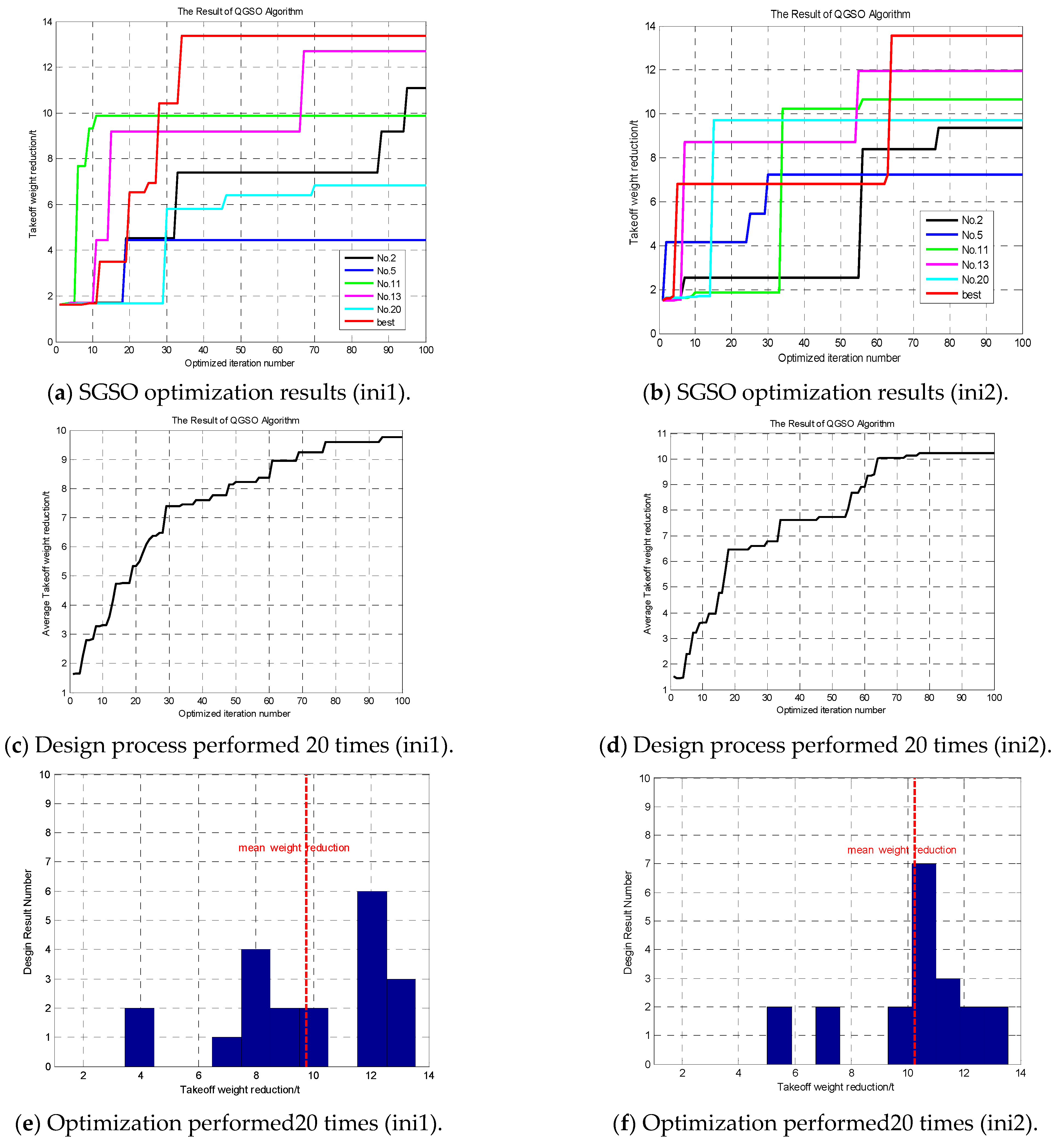
• A SGSO optimization method is used to optimize the proposed three-stage launch approach. In order to enhance the spatial coverage efficiency of the individual glowworm population, a quantum coding is applied into the SGSO algorithm to achieve glowworm encoding and parallel computing. This QGSO algorithm yields a better convergence speed and improved global exploration ability;
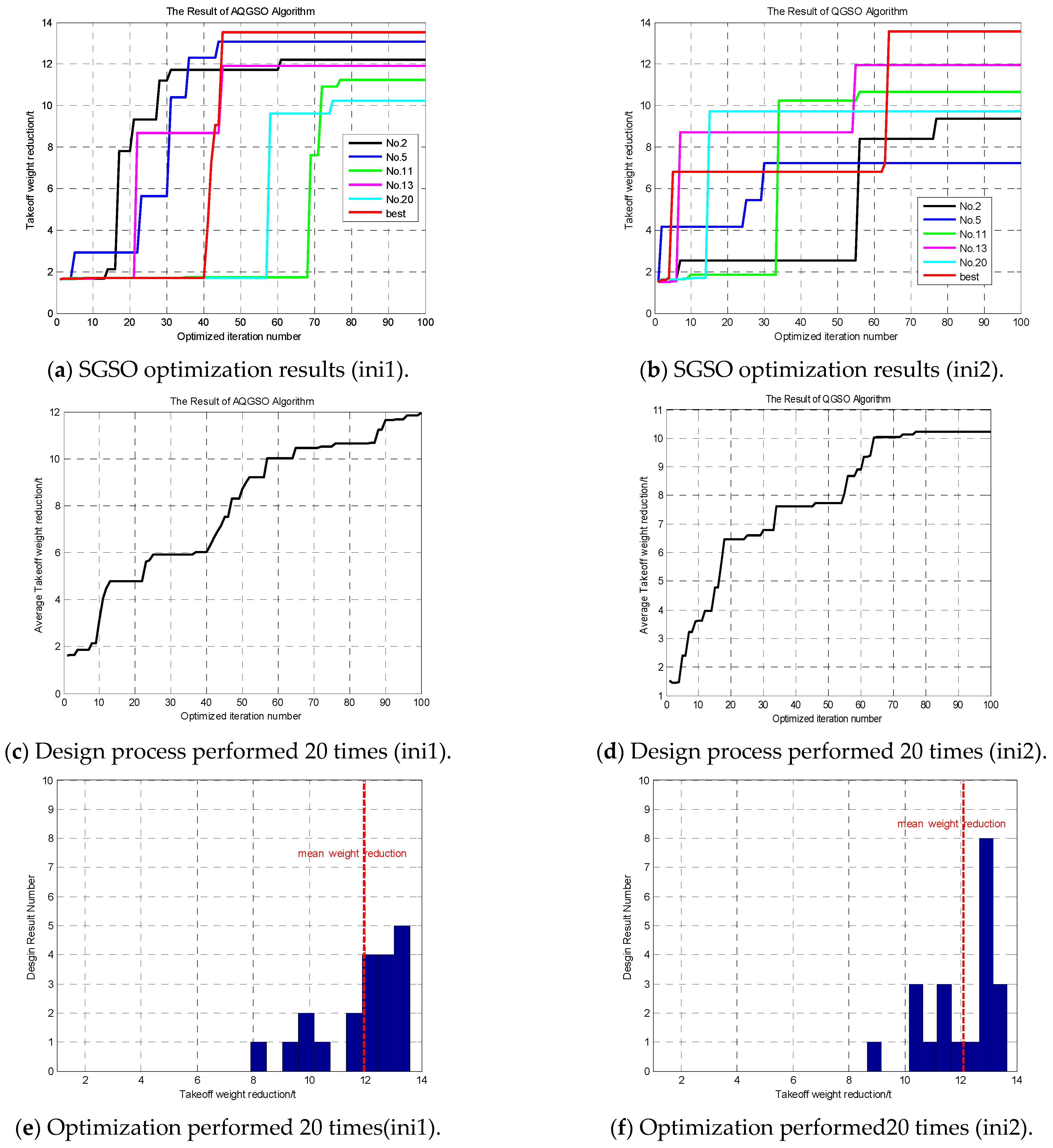
• For the nonlinearity and complexity of the proposed EMB system, a parameters sensitivity analysis is performed. This sensitivity analysis provides insights into the influence of different parameters on EMB performance. In addition, based on these quantitative analysis results, a gradient-based adaptive step size adjustment strategy is developed. The robustness performance can be further improved using this AQGSO; the standard deviation is 41.86% lower than that of QGSO and 67.7% lower than that of SGSO.

By using the proposed orbital launch system and the optimization approach, a spacecraft with more space and capacity can be launched. The proposed novel three-level orbital launch approach provides fast deployment and effective implementation for the EMB system, which can help engineers to design and optimize the orbital launch system in the field of energy management and efficiency.

In future work, multi-level orbital systems will be further studied by combining other electromagnetic boosting forms, such as multi-pole electromagnetic boosting technology as a new type of electromagnetic launching technology. Compared with traditional inductive electromagnetic launching technology, this new method offers a large thrust, stable suspension, and a controllable torsional magnetic field, as well as good space application potential for large mass, large diameter projectiles and high-speed launching.

References

1. Ferrero, A.; Conte, A.; Martelli, E.; Nasuti, F.; Pastrone, D. Dual-bell nozzle with fluidic control of transition for space launchers. Acta Astronaut. 2022, 193, 130–137. [Google Scholar] [CrossRef]
2. Guadagnini, J.; Lavagna, M.; Rosa, P. Model predictive control for reusable space launcher guidance improvement. Acta Astronaut. 2021, 193, 767–778. [Google Scholar] [CrossRef]
3. Li, C.; Xia, Z.; Ma, L.; Zhao, X.; Chen, B.; Feng, Y.; Yang, P. Experimental investigation on the ignition delay of fuel-rich mixture in solid rocket scramjet. Acta Astronaut. 2021, 190, 112–117. [Google Scholar] [CrossRef]
4. Jo, B.-U.; Ahn, J. Optimal staging of reusable launch vehicles for minimum life cycle cost. Aerosp. Sci. Technol. 2022, 127, 107703. [Google Scholar] [CrossRef]
5. Zhang, T.; Yan, X.; Huang, W.; Che, X.; Wang, Z. Multidisciplinary design optimization of a wide speed range vehicle with waveride airframe and RBCC engine. Energy 2021, 235, 121386. [Google Scholar] [CrossRef]
6. Shi, G.; Zhu, Z.H.; Li, G. Stable cargo transportation of partial space elevator with multiple actuators. Adv. Space Res. 2021, 68, 2999–3011. [Google Scholar] [CrossRef]
7. Lei, B.; Zhang, M.; Lin, H.; Nie, H. Optimization design containing dimension and buffer parameters of landing legs for reusable landing vehicle. Chin. J. Aeronaut. 2021, 35, 234–249. [Google Scholar] [CrossRef]
8. Luo, S.; Wu, X.; Wei, C.; Zhang, Y.; Yang, Z. Adaptive finite-time prescribed performance attitude tracking control for re-usable launch vehicle during reentry phase: An event-triggered case. Adv. Space Res. 2022, 69, 3814–3827. [Google Scholar] [CrossRef]
9. Karas, V.; Zajaček, M.; Kunneriath, D.; Dovčiak, M. Electromagnetic signatures of strong-field gravity from accreting black-holes. Adv. Space 2022, 69, 448–466. [Google Scholar] [CrossRef]
10. Qi, D.; Yang, L.; Zhu, Y.; Zhang, Y.; Li, Y. Optimal reconfigurations between equilibria of two-craft electromagnetic for-mations along manifolds. Aerosp. Sci. Technol. 2018, 79, 531–542. [Google Scholar] [CrossRef]
11. Guillot, M.J.; McNab, I.R. Aerothermal Analysis of Small Payloads delivered into Low Earth Orbit from an Airborne Launch Platform. In Proceedings of the AIAA Summer Heat Transfer Conference, Paper HT2008-56438, Jacksonville, FL, USA, 10–14 August 2008. [Google Scholar]
12. Deng, C.; Ye, C.; Yang, J.; Sun, S.; Yu, D. Electromagnetic Augmentation can reduce Space Launch Costs. IEEE Trans-Actions Appl. Supercond. 2020, 30, 19642969. [Google Scholar]
13. Mcnab, I.R.; Wolfe, T.R. Electromagnetic Launch to Space. J. Br. Interplanet. Soc. 2018, 115, 1066–1068. [Google Scholar]
14. Inger, E. Electromagnetic Launching Systems to Geosynchronously Equatorial Orbit in Space and Cost Calculations. IEEE Trans. Plasma Sci. 2017, 45, 1663–1666. [Google Scholar] [CrossRef]
15. Xinpeng, X.; Tao, S.; Zhiyong, Y.; Gang, F. Design of Multipole Electromagnetic Emitter for Surface-to-air Missile. J. Proj. Rocket. Missiles Guid. 2017, 37, 27–31. (In Chinese) [Google Scholar]
16. Gao, M.; Wang, Y.; Wang, Y.; Wang, P. Experimental investigation of non-linear multi-stable electromagnetic-induction energy harvesting mechanism by magnetic levitation oscillation. Appl. Energy 2018, 220, 856–875. [Google Scholar] [CrossRef]
17. Klinar, K.; Tomc, U.; Jelenc, B.; Nosan, S.; Kitanovski, A. New frontiers in magnetic refrigeration with high oscillation energy-efficient electromagnets. Appl. Energy 2019, 236, 1062–1077. [Google Scholar] [CrossRef]
18. Halim, M.; Rantz, R.; Zhang, Q.; Gu, L.; Yang, K.; Roundy, S. An electromagnetic rotational energy harvester using sprung eccentric rotor, driven by pseudo-walking motion. Appl. Energy 2018, 217, 66–74. [Google Scholar] [CrossRef]
19. Yeong, S.P.; Law, M.C.; You, K.Y.; Chan, Y.S.; Lee, V.C. A coupled electromagnetic-thermal-fluid-kinetic model for microwave-assisted production of Palm Fatty Acid Distillate biodiesel. Appl. Energy 2019, 237, 457–475. [Google Scholar] [CrossRef]
20. Krishnanand, K.; Ghose, D. Glowworm swarm based optimization algorithm for multimodal functions with collective robotics applications. Multiagent Grid Syst. 2006, 2, 209–222. [Google Scholar] [CrossRef]
21. Krishnanand, K.N.; Ghose, D. Glowworm swarm optimisation: A new method for optimising multi-modal functions. Int. J. Comput. Intell. Stud. 2009, 1, 93–119. [Google Scholar] [CrossRef]
22. Wang, X.; Zhang, H.; Bai, S.; Yue, Y. Design of agile satellite constellation based on hybrid-resampling particle swarm optimization method. Acta Astronaut. 2021, 178, 595–605. [Google Scholar] [CrossRef]
23. Marinaki, M.; Marinakis, Y. A Glowworm Swarm Optimization algorithm for the Vehicle Routing Problem with Stochastic Demands. Expert Syst. Appl. 2016, 46, 145–163. [Google Scholar] [CrossRef]
24. Yang, B.; Wu, S.; Zhang, H.; Liu, B.; Shu, H.; Shan, J.; Ren, Y.; Yao, W. Wave energy converter array layout optimization: A critical and comprehensive over-view. Renew. Sustain. Energy Rev. 2022, 167, 112668. [Google Scholar] [CrossRef]
25. Pruthi, J.; Khanna, K.; Arora, S. Optic Cup segmentation from retinal fundus images using Glowworm Swarm Optimization for glaucoma detection. Biomed. Signal Process. Control 2020, 60, 102004. [Google Scholar] [CrossRef]
26. Wang, X.; Yang, K. Economic load dispatch of renewable energy-based power systems with high penetration of large-scale hydropower station based on multi-agent glowworm swarm optimization. Energy Strat. Rev. 2019, 26, 100425. [Google Scholar] [CrossRef]
27. Braik, M.; Hammouri, A.; Atwan, J.; Al-Betar, M.A.; Awadallah, M.A. White Shark Optimizer: A novel bio-inspired meta-heuristic algorithm for global optimization problems. Knowl.-Based Syst. 2022, 243, 108457. [Google Scholar] [CrossRef]
28. Mojrian, M.; Mirroshandel, S.A. A novel extractive multi-document text summarization system using quantum-inspired genetic algorithm: MTSQIGA. Expert Syst. Appl. 2021, 171, 114555. [Google Scholar] [CrossRef]
29. Szwarcman, D.; Civitarese, D.; Vellasco, M. Quantum-inspired evolutionary algorithm applied to neural architecture search. Appl. Soft Comput. 2022, 120, 108674. [Google Scholar] [CrossRef]
30. Grossi, F.; Circi, C. Quantum-inspired diffusion Monte Carlo optimization algorithm applied to space trajectories and attitude maneuvers. Adv. Space Res. 2022, 69, 592–608. [Google Scholar] [CrossRef]
31. Ding, S.; Zhang, Z.; Sun, Y.; Shi, S. Multiple birth support vector machine based on dynamic quantum particle swarm optimization algorithm. Neurocomputing 2022, 480, 146–156. [Google Scholar] [CrossRef]
32. Xin, G.; Wang, P. Exploring superposition state in multi-scale quantum harmonic oscillator algorithm. Appl. Soft Comput. 2021, 107, 107398. [Google Scholar] [CrossRef]
33. Xin, G.; Wang, P.; Jiao, Y. Multiscale quantum harmonic oscillator optimization algorithm with multiple quantum per-turbations for numerical optimization. Expert Syst. Appl. 2021, 185, 115615. [Google Scholar] [CrossRef]
34. Yazhong, J.; Chongwen, J.; Zhenxun, G.; Chunhian, L. Mass estimation method and its application for hori-zontal takeoff horizontal landing two stage to orbit system. J. Beijing Univ. Aeronaut. Astro-Naut. 2014, 40, 473–478. [Google Scholar]
35. Siebenhaar, A.; Bulman, M.J. The Strutjetrocket Based Combined Cycle Engine; NAS8-40891; NTRS: New York, NY, USA, 1999. [Google Scholar]
36. Zhou, D.; Nguyen, T.T.; Breaz, E.; Zhao, D.; Clénet, S.; Gao, F. Global parameters sensi-tivity analysis and development of a two-dimensional real-time model of proton-exchange-membrane fuel cells. Energy Convers. Manag. 2018, 162, 276–292. [Google Scholar] [CrossRef]
Figure 1. Motivation for the proposed launch approach based on EMB and the optimization algorithm.
Energies 16 07717 g001
Figure 2. Three-stage-to-orbit reusable vehicle launch system.
Energies 16 07717 g002
Figure 3. The schematic diagram of the TBCC-RR vehicle mission profile.
Energies 16 07717 g003
Figure 4. Schematic diagram of the EMB system.
Energies 16 07717 g004
Figure 5. The schematic diagram of the equivalent circuit model for the EMB system.
Energies 16 07717 g005
Figure 6. Take-off weight estimation model of a reusable vehicle based using EMB-TBCC-RR.
Energies 16 07717 g006
Figure 7. Maxwell structure of EMB system.
Energies 16 07717 g007
Figure 8. Mutual induction and its fitted curve.
Energies 16 07717 g008
Figure 9. The electromagnetic force and velocity of the armature of the single stage EMB.
Energies 16 07717 g009
Figure 10. The armature velocity of a multiple stage EMB system.
Energies 16 07717 g010
Figure 11. Schematic diagram of take-off weight optimization based on the cluster intelligent algorithm.
Energies 16 07717 g011
Figure 12. Sensitivity analysis results for different selected five parameters.
Energies 16 07717 g012
Figure 13. SGSO algorithm optimized design results.
Energies 16 07717 g013aEnergies 16 07717 g013b
Figure 14. Optimization results of QGSO algorithm.
Energies 16 07717 g014
Figure 15. Optimization results for the AQGSO algorithm.
Energies 16 07717 g015