Article

Analysis of Air Pollutants for a Small Paintshop by Means of a Mobile Platform and Geostatistical Methods †

1
Faculty of Environmental Engineering, Wroclaw University of Science and Technology, Plac Grunwaldzki 13, 50-377 Wroclaw, Poland
2
Faculty of Architecture, Civil and Environmental Engineering, Łódź University of Technology, Al. Politechniki 6, 90-924 Łódź, Poland
3
Faculty of Physics and Applied Computer Science, Department of Applied Nuclear Physics, AGH University of Kraków, 30-059 Kraków, Poland
*
Author to whom correspondence should be addressed.
This paper is an extended version of our abstract published in Sówka, I.; Cichowicz, R.; Dobrzański, M.; Bezyk, Y. Application of mobile platform and geostatistical methods in the analysis of air quality in the selected area of the city of Lodz. In 4th Symposium “Air Quality and Health”; Korzystka-Muskała, M., Kubicka, J., Sawiński, T., Drzeniecka-Osiadacz, A., Eds.; University of Wrocław: Wrocław, Poland, 2023; pp. 94–95.
Energies 2023, 16(23), 7716; https://doi.org/10.3390/en16237716
Submission received: 12 September 2023 / Revised: 11 November 2023 / Accepted: 20 November 2023 / Published: 22 November 2023
(This article belongs to the Special Issue Selected Papers from the 16th Conference 'Air, Heat and Energy')

Abstract

:
Air pollution, in terms of particulate matter (PM10, PM2.5, PM1.0) and gaseous pollutants (H2S and VOC), has serious health effects, particularly in cities. The evaluation of outdoor air quality was carried out in the vicinity of a small paintshop operating in the city of Łódź, Poland. The concentrations of pollutants in the vertical profiles (up to 47 m a.g.l.) of ambient air were measured using a mobile platform (unmanned aerial vehicle with measuring equipment) during three measurement campaigns in September 2021. The vertical structure of the pollutant concentrations indicated the occurrence of different types of layers with an almost constant concentration near the land surface, a strong decrease (up to ca. 10–15 m a.g.l.), and significant fluctuations in concentrations to higher levels (above 25 m a.g.l.). Particulate matter concentrations (PM10, PM2.5, PM1.0) did not exceed 39 µg m−3, with stable levels on the surface. The maximum value of particulate matter concentrations (up to 38.5 µg m−3) in the vertical profiles was recorded at ca. 35–40 m a.g.l. The average concentrations of H2S and VOC varied between 0.07 and 0.12 ppm and 0.01 and 0.27 ppm, respectively. The highest H2S concentrations were observed at ca. 18–23 m a.g.l., reaching 0.14 ppm. A rapid increase in VOC concentrations, reaching 0.29 ppm, was measured in vertical profiles from 20 m a.g.l. and up to about 40 m a.g.l. In situ measurement approaches were combined with interpolation methods in the GIS system to investigate the spatial variability of pollution levels from a specified source in the urban atmosphere. Based on the survey results, the kriging interpolation method was well suited for generating spatially distributed pollution maps for individual measurement campaigns.

1. Introduction

Particulate matter and volatile organic compounds (VOCs) are hazardous pollutants emitted from various sources, such as from petroleum/solvent production activities, combustion processes, industrial and automobile emissions, paint and other solvents, aerosol sprays, building and construction materials [1]. Hydrogen sulfide (H2S) is regulated in many countries as it acts as a precursor of reduced sulfur and can affect plant development and cause significant negative effects on human health [2,3]. According to the guidelines of the World Health Organization, the maximum allowable level for the mean annual concentration of PM10 is 15 µg m−3, and 5 µg m−3 for PM2.5, while the 24 h PM10 standard is 45 µg m−3 and should not exceed 15 µg m−3 for PM2.5 more than 3–4 days per year [4]. The basic limit for the concentration of hydrogen sulfide (H2S) in air was determined to be 7 µg m−3 for an 8 h total weight average (TWA) [5]. The EU air quality standards for particulate matter and certain gaseous pollutants, reported under Directive 2008/50/EC on ambient air quality and cleaner air for Europe, aim to align EU air quality standards more closely with WHO recommendations. The EU Air Quality Directive sets objectives for ambient air quality and common methods for monitoring and assessing air pollutants and reducing risks to human health [6]. The effects of painting and coating operations on local air quality pose risks to public health. There have been a number of studies on outdoor air quality in urban areas and its effects on comfort and human health [1,7,8]. Thus, the ability to identify sources of air pollutant emissions and quickly assess air quality in urban areas, characterized by complex emission profiles, taking into account the dynamics of air pollutant distribution, becomes crucial. In this type of research, mobile platforms can be used in addition to measurements made as part of standard monitoring [9,10,11,12,13,14], and mobile measurement systems based on optical or electrochemical measurement sensors have been developed [15,16,17]. The miniaturization of the sensors allows them to be mounted on unmanned aerial vehicles [18,19,20]. Regarding the function of the carriers of the measurement apparatus, the best are multi-rotor drones, which allow flight and hovering in the air at any height in difficult urbanized and industrial terrain [9]. The available literature outlines several directions for the development of mobile air quality analysis technologies. These begin with research and attempts using drone-based construction and measurement apparatus [21,22], through the use of commercial solutions [23], and finally reach comprehensive approaches to the problem, consisting of the collection of measurement data using unmanned aerial vehicles, the processing of 3D data, and their analysis in GIS programs [20].
The GIS environment is often used for the monitoring, mapping and spatial analysis of air pollution, as well as to improve poor observation datasets and for geographical-based source identification [24,25,26]. Based on GIS tools, the results of in situ measurements can be represented as data interpretation and visualization-related time series of air pollutant concentrations [27,28]. The GIS interpolation techniques allow the prediction of unknown values at unsampled points based on the given points with known values distributed over the study area [27,29]. GIS spatial interpolation methods have been applied to many disciplines and different fields, e.g., natural resource and environmental management, geochemistry, urban planning, atmospheric and climate studies, meteorological data analysis, pollution transport modelling and health sciences [30,31]. The various spatial interpolation techniques perform differently depending on the nature of the inputs, the point density and configuration of the sampling locations and the spatial resolution characteristics [27,32]. In general, accurately interpolated surfaces are obtained when datasets are used that contain a sufficient number of sampling points that are sufficiently dense and sufficiently uniform (evenly or highly distributed) across the study area [27,33]. Spatial optimization and validation procedures of interpolation results can improve model prediction capabilities, depending on the spatial scale and geospatial characteristics of emissions and local meteorological conditions [34,35]. In addition, well-planned in situ measurements at the urban scale, focusing on the spatial and temporal patterns of pollutants, will help to constrain emissions and develop further mitigation options.
The objective of this study was to investigate air quality in the vicinity of a small paintshop operating in the city of Łódź (Poland), using a mobile platform (unmanned aerial vehicle with measuring equipment). Research addresses the issues in concentration measurements of particulate matter (PM10, PM2.5, PM1.0) and gaseous pollutants (H2S, and VOC) above ground level, using the spatial interpolation technique for air quality mapping. Local-scale spatial and temporal information on pollution levels could also help to characterize possible environmental effects and health risks, to produce a background for modelling studies, and to provide guidance for future sampling strategies.

2. Materials and Methods

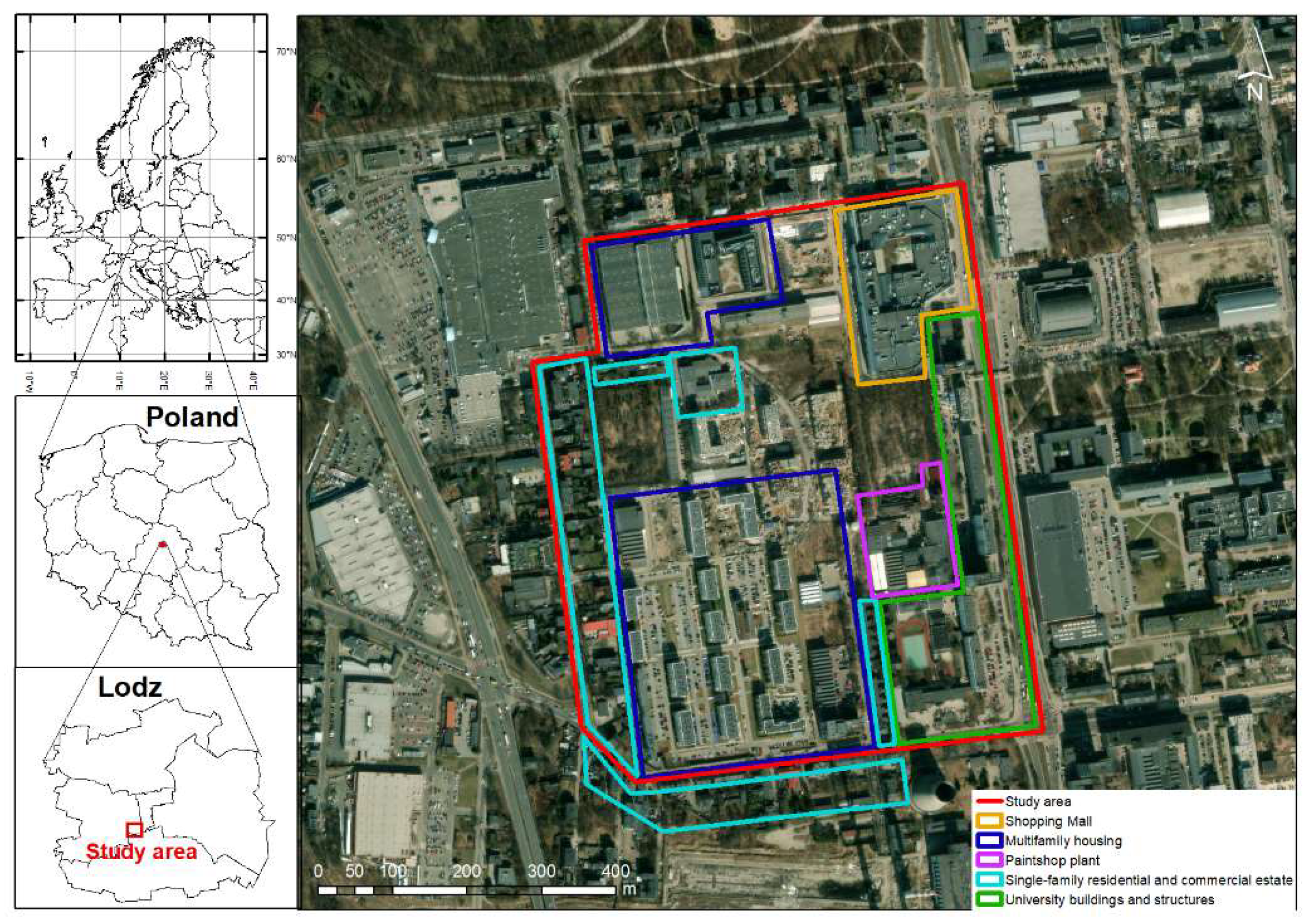
2.1. Site Description

The research site is located in the city of Łódź in central Poland (Figure 1). Łódź is the fourth-largest city in Poland, with a population of 6,767,923 in 2021 [36] and an area of 293.25 km2 [37]. Historically, the Łódź voivodship and the Łódź agglomeration itself have been associated with the textile industry. At present, however, the share of this industry has decreased in favor of an increase in the importance of the energy, engineering, agro-food, metallurgical, pharmaceutical and construction industries. The fact that the voivodeship is well connected to the rest of the country by motorways and expressways has led to the establishment of many forwarding companies and distribution centers. The main products of the region are ceramic tiles, household appliances, cotton fabrics, brown coal, electricity, food and beverages, rubber products and plastics. There are significant differences in the degree of industrialization between the counties. In addition to industrial areas such as the city of Łódź and the Pabianicki and Zgierz counties, there are typically agricultural counties, such as Łęczycki, Sieradzki, Poddębicki and Wieruszowski. The main sources of air pollution in the Łódź voivodeship are anthropogenic emissions from the residential sector from individually heated houses (responsible for PM10, PM2.5 and benzo(a)pyrene), from communication and road traffic (NOx, PM10 and PM2.5) and from commercial power generation (SOx and NOx). Other local sources include heaps, pits, composting plants, landfills and sewage treatment plants. A significant amount of the air pollutant concentrations in the area of the voivodship are due to their inflow from the rest of Poland [38].
The climate of Łódź is characterized as humid-continental, with cold winters and warm summers [40]. The average annual temperature (for the years 1991–2020) was 9 °C, with the highest temperatures observed in July and the minimum usually recorded in January [39]. The annual sum (average for the years 1991–2020) of atmospheric precipitation was 712 mm [41]. More than 37% of the rainfall occurs during summer (in the range of 60 to 80 mm), and the lowest precipitation amount recorded falls from December to February (from 30 to 40 mm) [42]. The prevailing winds were from the western direction (W, WSW, SW) and their average speeds at a height of 10 m a.g.l. were 4–6 m·s–1 [43]. The wind direction and wind velocity data for the city of Łódź in 2021 are shown in Figure 2.
The area selected for analysis, covering 42 hectares, is located in the southwestern part of downtown Łódź (Figure 1). The altitude of the study area varies from 187 to 189 m a.s.l. The building intensity index ranges from 0.5 to 1.0, and is characteristic of urban development. Within a radius of 300 m from the study site, there are tall buildings ranging in height from 15 to 30 m (Table 1). To the north, the paint shop is surrounded by a wooded park of a height up to 14 m. The tallest building (up to 120 m above sea level), located to the south (about 400 m) of the investigated plant, is a combined heat and power plant, currently in the process of being liquidated. Potential sources of high emissions in the city of Łódź are coal-fired power plants located far (~8 km) from the given facility in the north-western (EC-3) and eastern (EC-4) parts of the city.

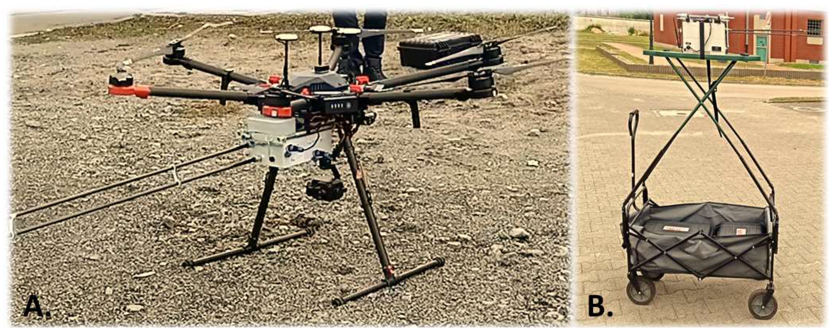
2.2. Sampling Methodology

We investigated the pollutant concentrations in vertical profiles (up to 47 m a.g.l.) near the paintshop during survey campaigns on 9, 16 and 23 September 2023 for the period from 09:00 to 10:00 UTC. Concentrations of particulate matter (PM10, PM2.5, PM1.0), volatile organic compounds (VOCs) and hydrogen sulfide (H2S) were measured simultaneously using an unmanned aerial vehicle (UAV) with installed measurement apparatus (GP) (Figure 3).
The UAV and GP measurement apparatus was equipped with the following sensors: a Laser Scattered (LS) sensor, where the module measured PM10, PM2.5 (10,000 particles per second); ElectroChemical (EC)-type sensors, which measured H2S (3 ppb to 1 ppm); and a Metal Oxide Semiconductor (MOS) type sensor: VOC (ethanol, isobutane, 0–500 ppm). The sampling frequency of each sensor module was (1) 2 Hz and a resolution of 1 µg/m3 for the Laser Scattered (LS) sensor; (2) 2 Hz and a resolution of 1 ppb for the ElectroChemical (EC) type sensor; and 2 Hz and a resolution of 0.1 ppm for the Metal Oxide Semiconductor (MOS) sensor. The UAV allowed measurements to be taken at heights ranging from 10 to 45 m a.g.l., whereas the GP was used to take measurements at a height of about 2 m a.g.l.
The measurement campaigns in this study were conducted under well-mixed conditions (from 9 a.m. to 12 p.m.) during three survey campaigns in September 2021 (time series from 9, 16 and 23 September 2021). The study period was selected to minimize the impact of individual heating systems on the measurement results during the cold season. The UAV flew in vertical profiles (up to 47 m a.g.l.) at a speed of 5.6 m s–1, providing measurements in a line with spacing of 25 m.

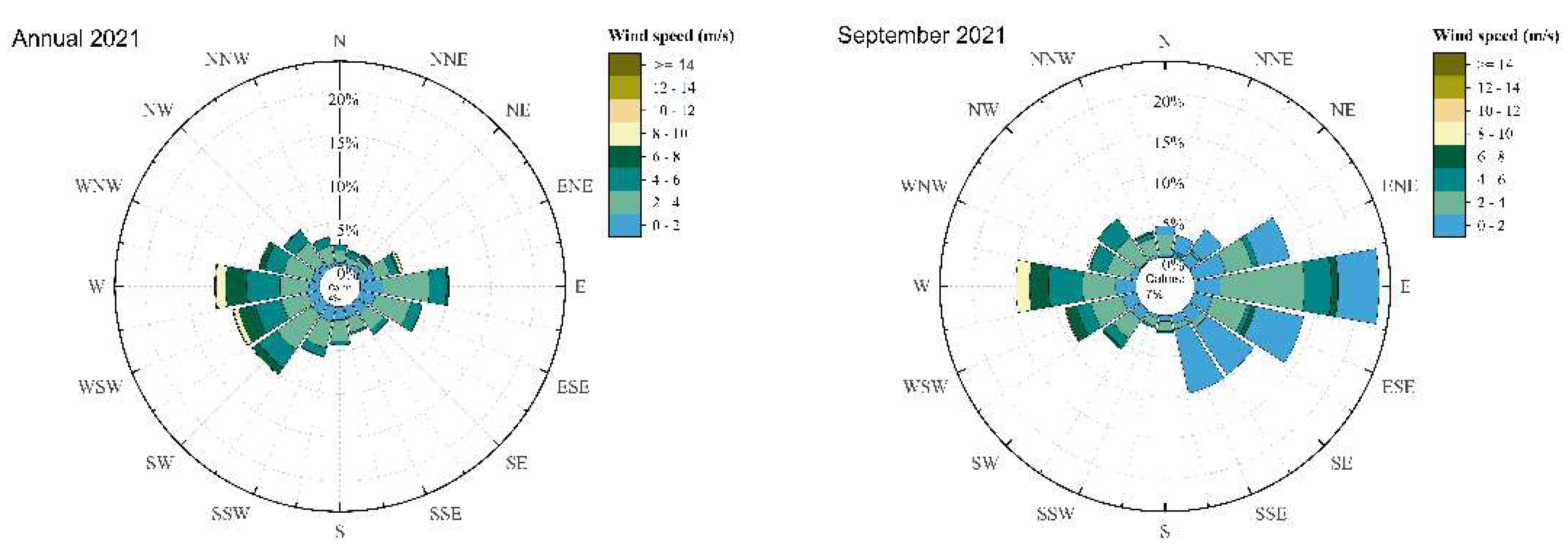
2.3. Meteorological Data
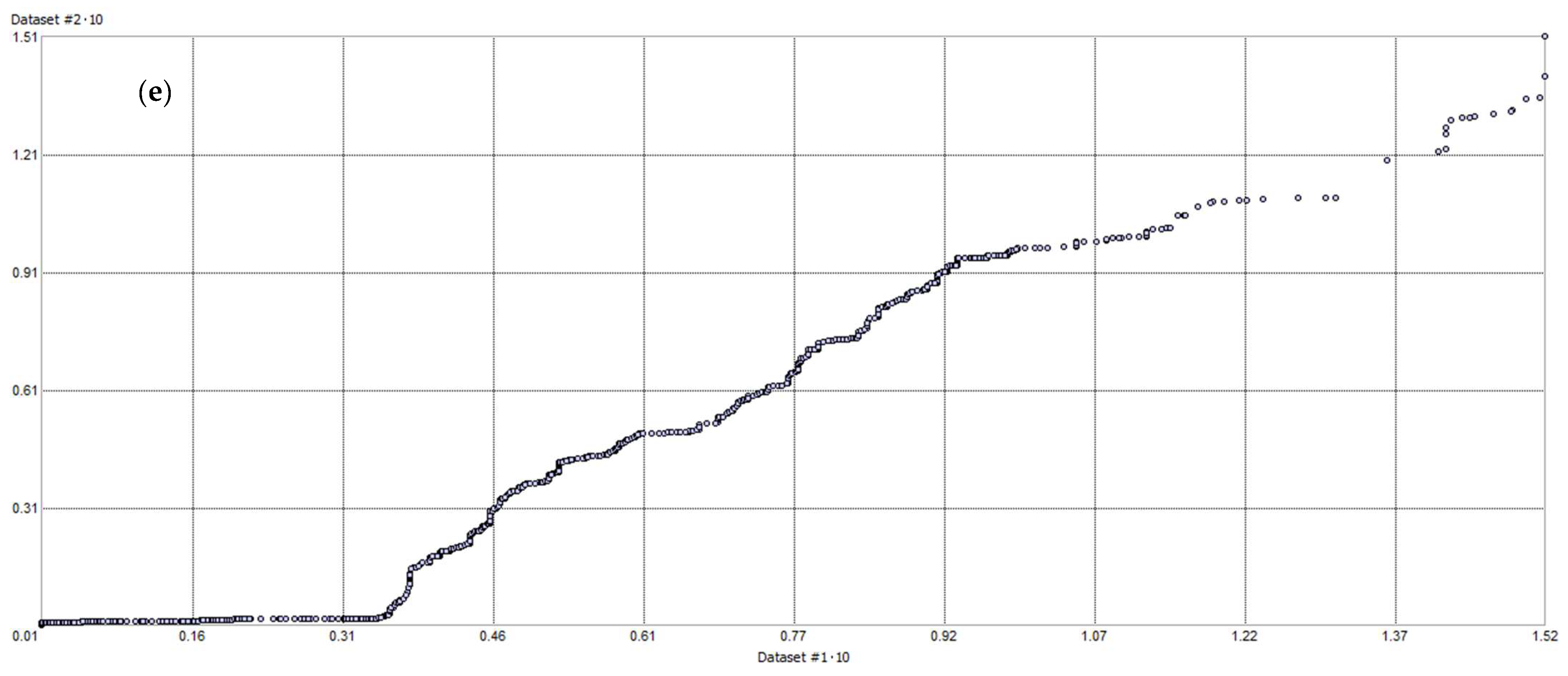
Weather parameters (barometric pressure, relative humidity, temperature, wind speed and direction) were measured during each sampling campaign using sensors installed on the UAV and at the surface meteorological station ‘Łódź-Lublinek’. Meteorological data obtained during these campaigns are presented in Table 2.

2.4. Data Analysis

The statistical analysis of the samples collected during the sampling campaigns and the measured meteorological parameters was performed using OriginPro 2021 software. Normality tests were carried out using Shapiro–Wilk estimates. Pearson’s correlation coefficient was used to test for possible relationships between the analyzed parameters.
In the current study, the performance of Ordinary Kriging interpolation to analyze the spatial and temporal variability of the measured pollution concentration in the vicinity of the paintshop was determined. The interpolated surfaces were generated using ArcGIS 10.8 software within the Spatial Analyst and the Geostatistical Analyst techniques in the Geostatistical Wizard extension. The sensitivity of each method to input data characteristics with different parameters (weights of the sample point structure, number of measured points of the search radius) was evaluated. The semivariance function was used to characterize the spatial continuity between points and to estimate the spatial dependence between observations.

3. Results and Discussion

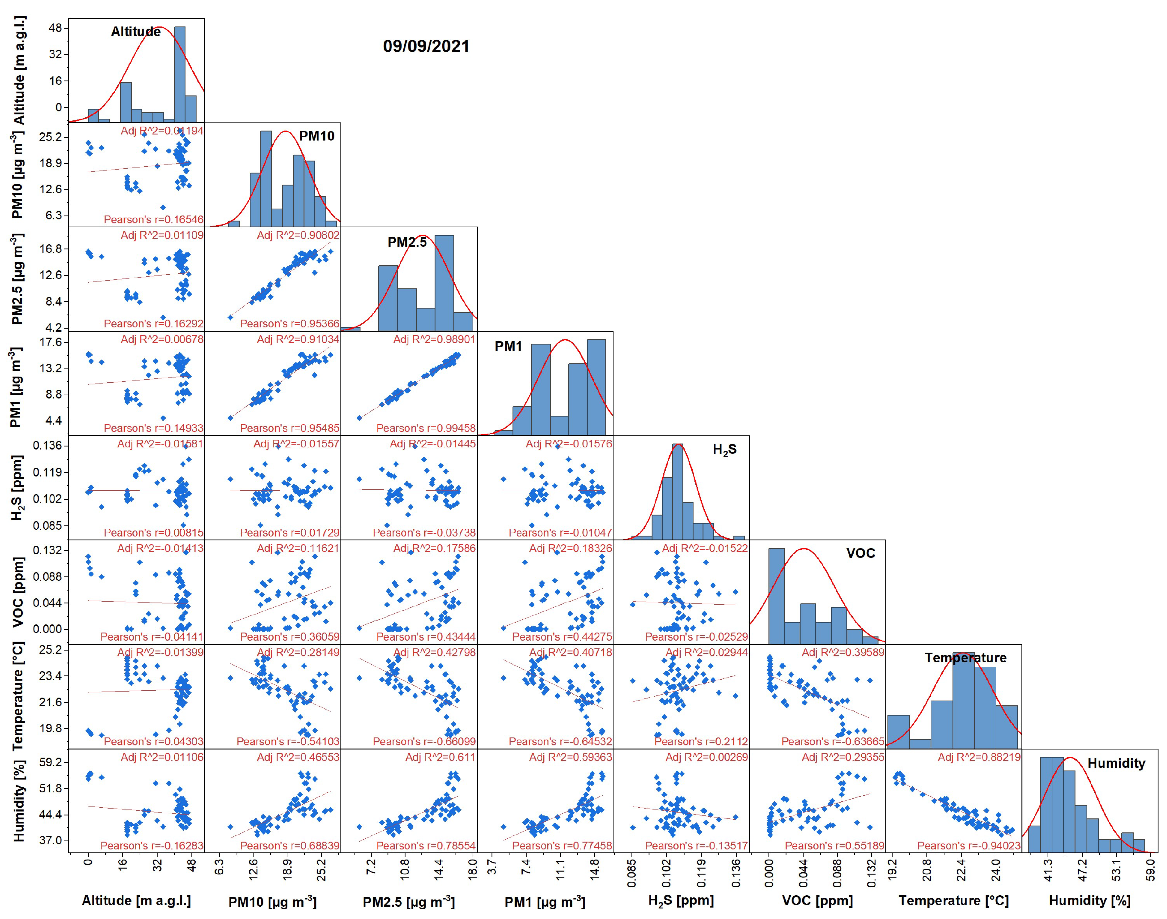
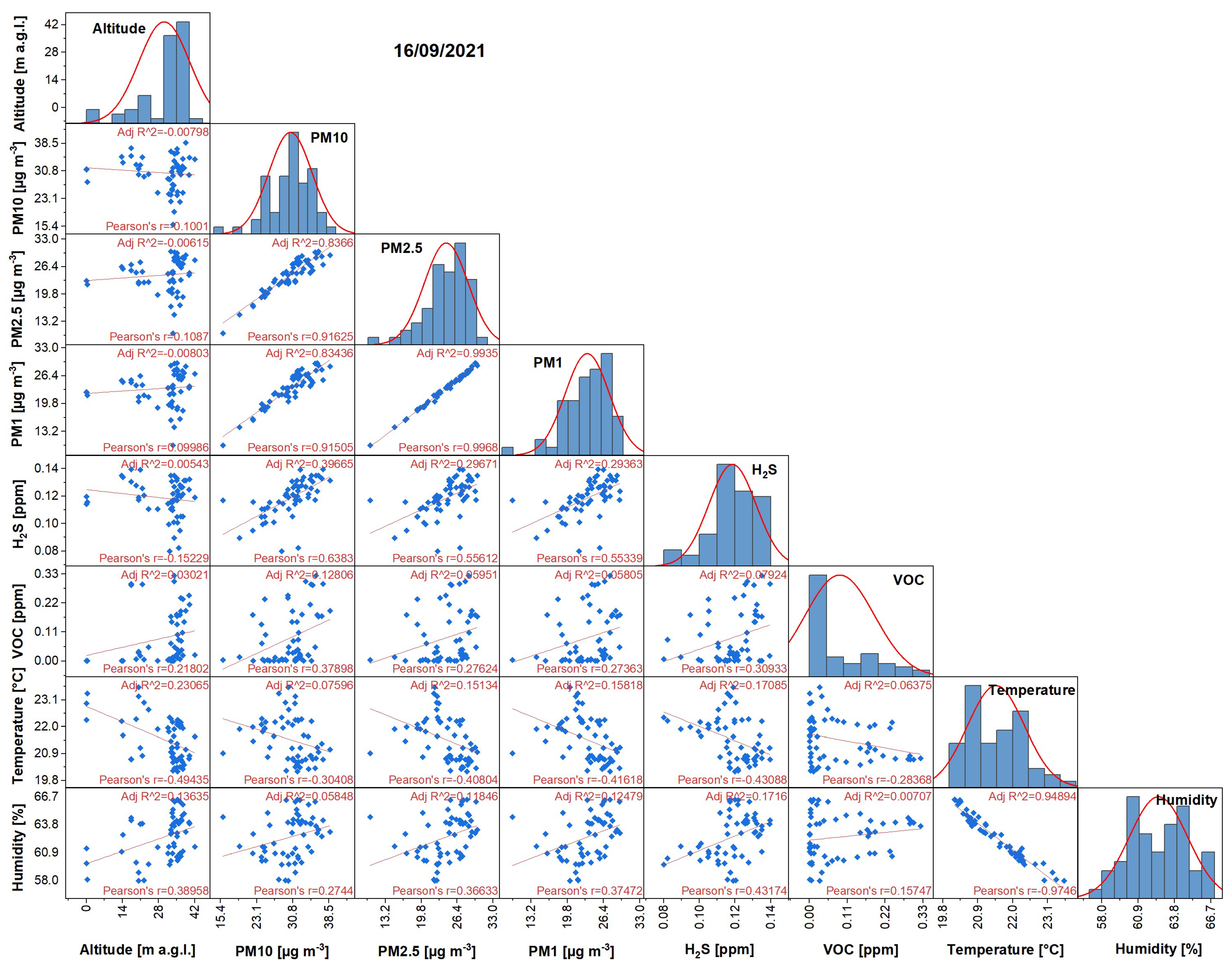
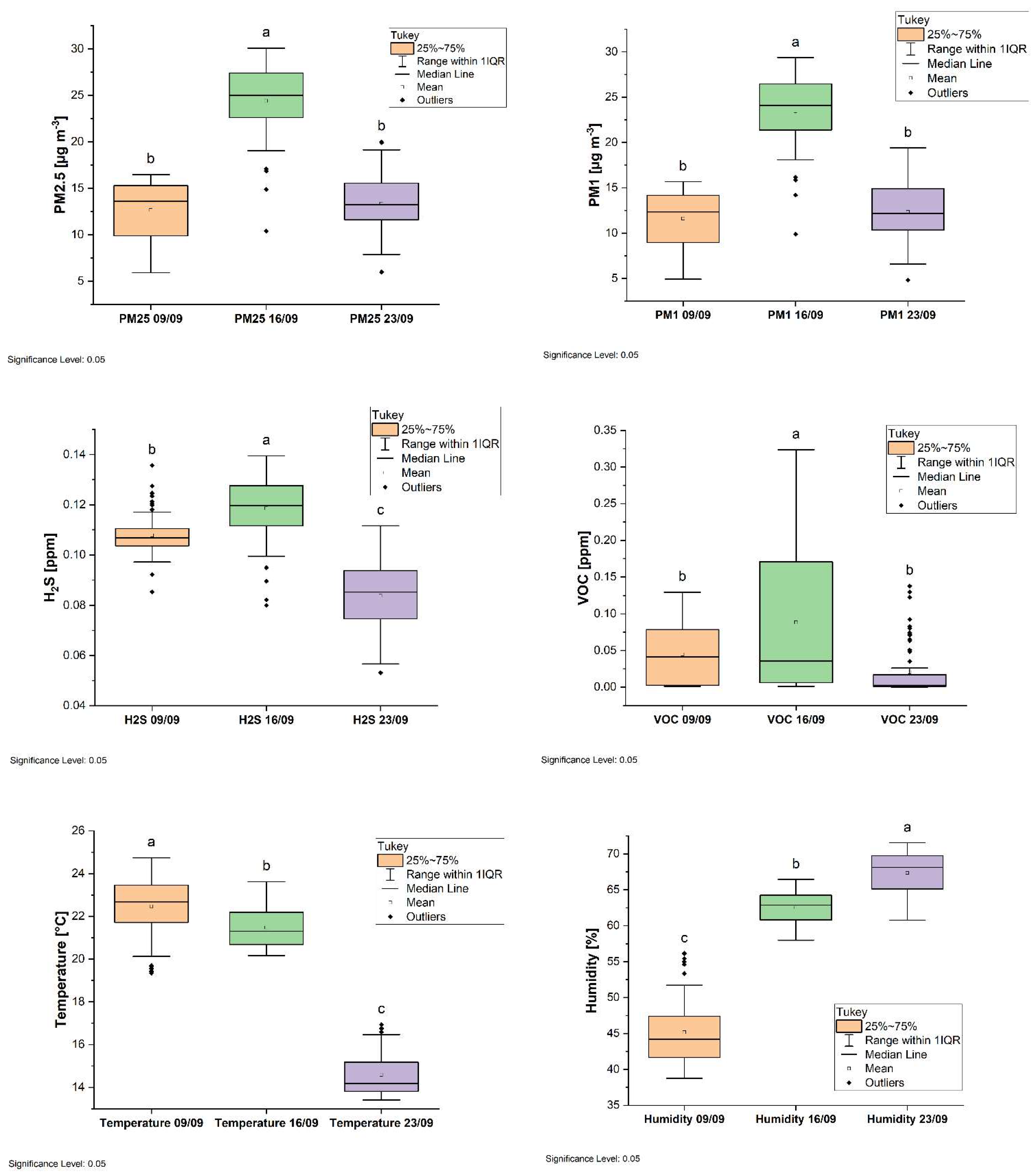
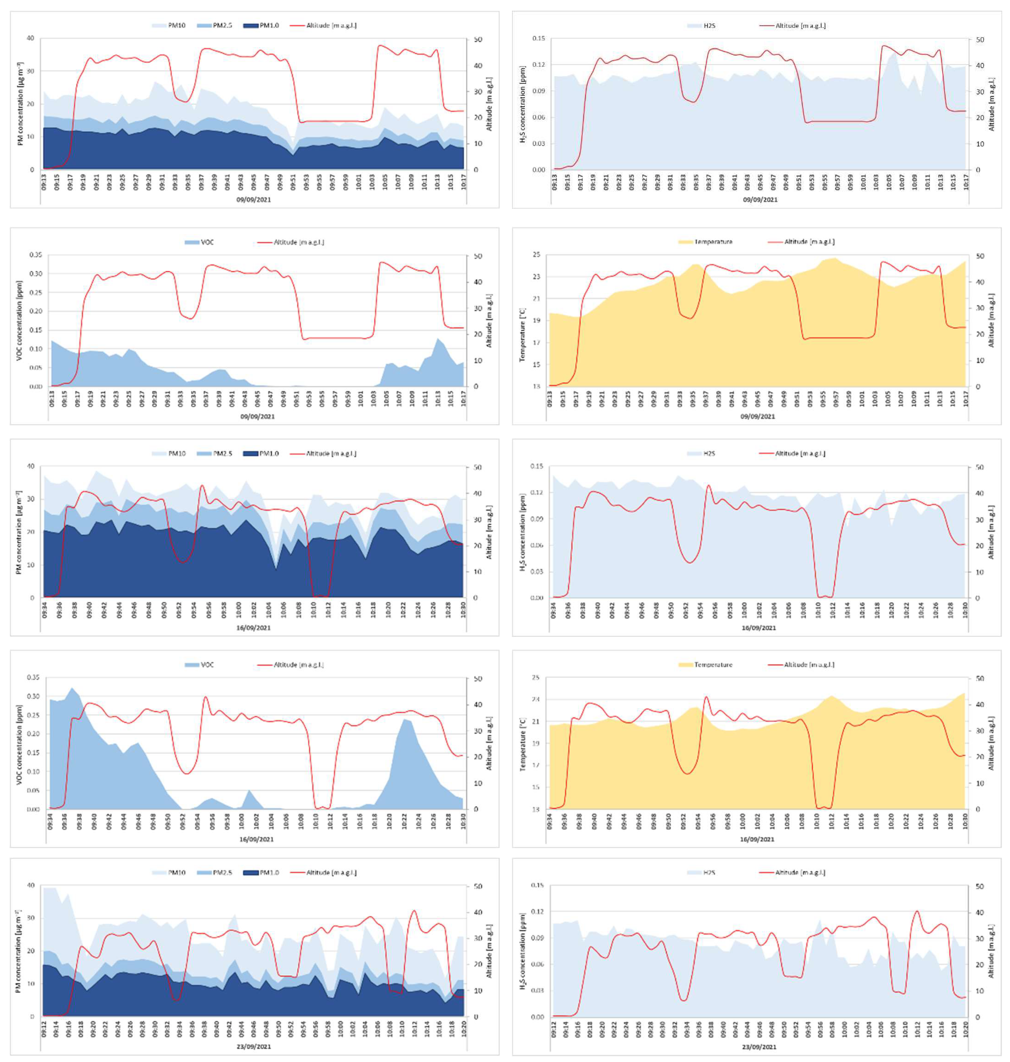
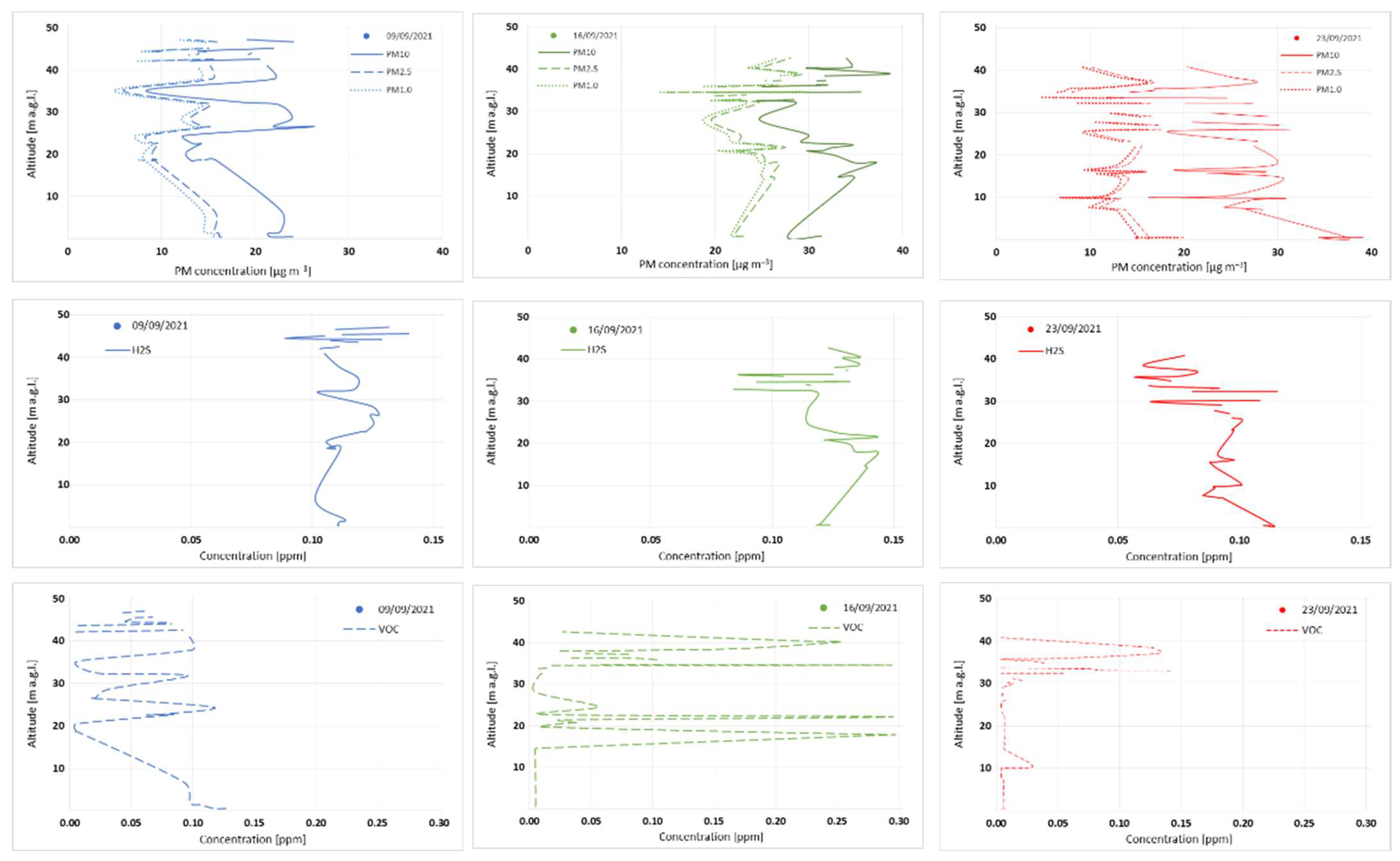
3.1. Analysis of the Measured Pollution Concentrations in Ambient Air

The measured patterns of atmospheric pollution concentrations for each sampling campaign were partly skewed compared with the normal distribution. The distribution of particulate matter (PM10, PM2.5 and PM1.0) showed a variable trend between sampling campaigns, with slight left-hand skewness (see Figure A1). The VOC distribution was more concentrated on one side of the scale, with a long tail on the right. Data showing a skewed distribution were logarithmically transformed prior to the statistical analysis (see Figure A1).
Temporal changes in meteorological parameters such as boundary layer height, wind speed and direction, temperature and relative humidity greatly influence the variability of pollution levels. In our study, the relationship between the pollutant concentrations and meteorological conditions in a short time series showed definite low values of correlation coefficients, suggesting possible narrow parameter variations in each campaign. The relationship between pollutant concentration and temperature showed a weak negative correlation with particulate matter (PM10, PM2.5 and PM1.0), H2S and VOC (r = –0.23 to –0.44, p = 0.05), as well as a positive correlation between pollutant concentrations and relative humidity (r = 0.13 to 0.45, p = 0.05). The Pearson correlation coefficient values were comparable between campaigns on 16 September 2021 and 23 September 2021; however, they were slightly different for measurements on 9 September 2021 (r = –0.54 to –0.66, p = 0.05 and r = 0.55 to 0.78, p = 0.05 for temperature and humidity, respectively) (see Figure A1 and Figure A2). The higher temperature and lower relative humidity on 9 September indicate a period of dry weather with relatively low wind speed.
An analysis of the vertical structure of the pollutant distribution revealed the occurrence of different types of layers. Short time changes are characterized by almost constant concentration at the ground level, with significant decreases up to ca. 10–15 m a.g.l. and higher concentrations at heights above 25 m a.g.l. (Figure 4). The mean concentration of particulates (PM10, PM2.5, PM1.0) was in the range of 15–30 µg m−3, reaching a maximum value of 39 µg m−3 at the ground level. At heights of 5 to 20 m, the average concentration of particulates ranged from 15 to 25 µg m−3. The highest value of particulates (up to 38.5 µg m−3) in vertical profiles was recorded at ca. 35–40 m a.g.l. There was a significant difference in the particulate matter concentration throughout the altitude profiles during the three survey campaigns in September 2021 (see Figure A2).
Measurements of H2S and VOC in the vertical profile indicated the high variability of the observed concentrations during each sampling campaign (Figure 5). The mean values of H2S and VOC varied between 0.07 and 0.12 ppm and 0.01 and 0.27 ppm, respectively. The highest H2S, reaching 0.14 ppm, was observed at ca. 18–23 m a.g.l., and was found on 16 September 2023. The average concentration of VOC was in the range of 0.05–0.10 ppm, with low and moderate variability in the time series from 9 and 23 September. The rise in VOC levels, which reached 0.29 ppm, was measured in vertical profiles of 20 m a.g.l. and up to about 40 m a.g.l. on 16 September 2023. During other sampling time series, the pollutant concentrations were about 20–40% lower (up to 0.14 ppm), which clearly showed that there was a significant difference between sampling sessions (see Figure A2).
Figure 4 shows the temporal variations in particulate matter (PM10, PM2.5 and PM1.0), H2S and VOC concentrations during the sampling campaign in the vicinity of a small paintshop. The pollutant levels showed similar vertical profiles, with concentrations nearly constant up to 15–20 m a.g.l, whereas the highest variation was observed when flying upward (peaking at a height of about 40 m a.g.l.). The vertical magnitude of pollutants at peak times can be explained by the impact of the main sources of air pollutants and/or transport processes, the dominant wind direction, and the dispersion conditions in the atmosphere (Figure 4). It is expected that the particles measured at the ground level and at a higher altitude were derived from road transport organized on a dense network of communication routes, as well as from the effect of air stagnation caused by the presence of buildings at the height of 6–11 stories (15–33 m) in the measurement area.
The measured concentrations of hydrogen sulfide and volatile organic compounds gradually increased along with the flight altitude, which likely resulted from the UAV flying in the spot where air pollutants were most concentrated. The repetitive patterns of increased concentrations of both H2S and VOC at higher altitudes (above 20 m a.g.l.) across the three sampling campaigns in September 2021 have generally been associated with enhanced chemical compound formation derived from paintshop operations. Furthermore, by revealing the peaks of levels of volatile organic compounds for each time series, it was identified that the paintshop is the main source of VOCs in the surrounding environment (Figure 4).
The vertical profile of atmospheric pollutants was examined using UAV measurements during various previous studies performed in the city of Łódź. As demonstrated by profiles obtained from previous UAV flights over urban agglomeration, the distributions of particulate matter (PM10, PM2.5 and PM1.0) and gaseous pollutants (H2S, SO2 and VOC) varied between low and high altitudes, industrial units and under different emission scenarios and meteorological conditions [10,45,46]. Generally, the results showed clear differences in terms of the distribution of pollutants, mainly caused by local sources and higher at a height of more than 40 m and/or accumulated near the ground level. Previous studies that examined the relationships between air pollution levels and industrial agglomeration factors detected an increase in their concentrations in the immediate vicinity of industrial areas, close to heat and power plants, and at the intersection of communication routes. This is consistent with our observations, in which high levels of pollutants were detected close to the industrial unit (paintshop), with peaks also occurring at a height of about 30–40 m a.g.l.

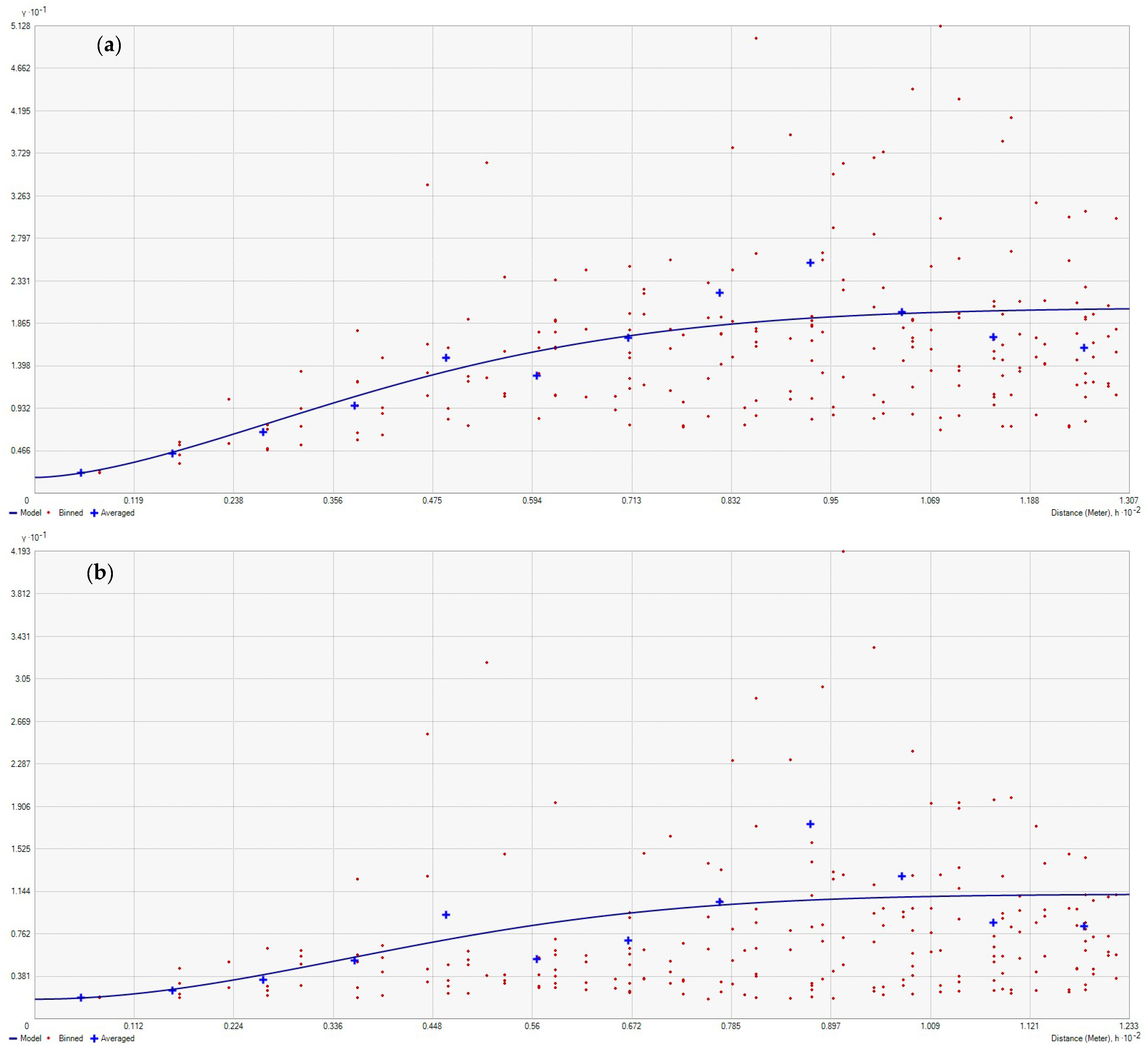
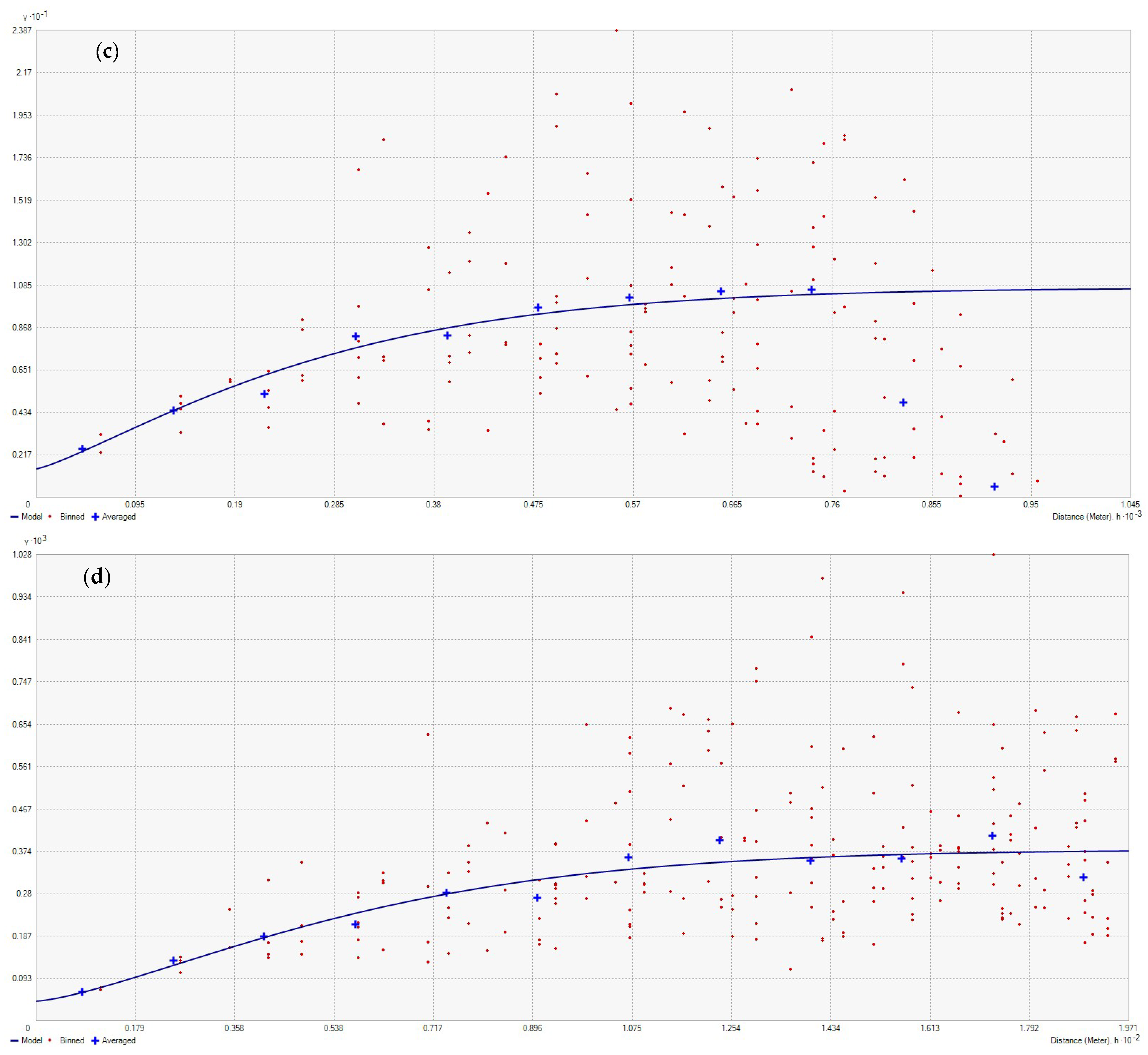
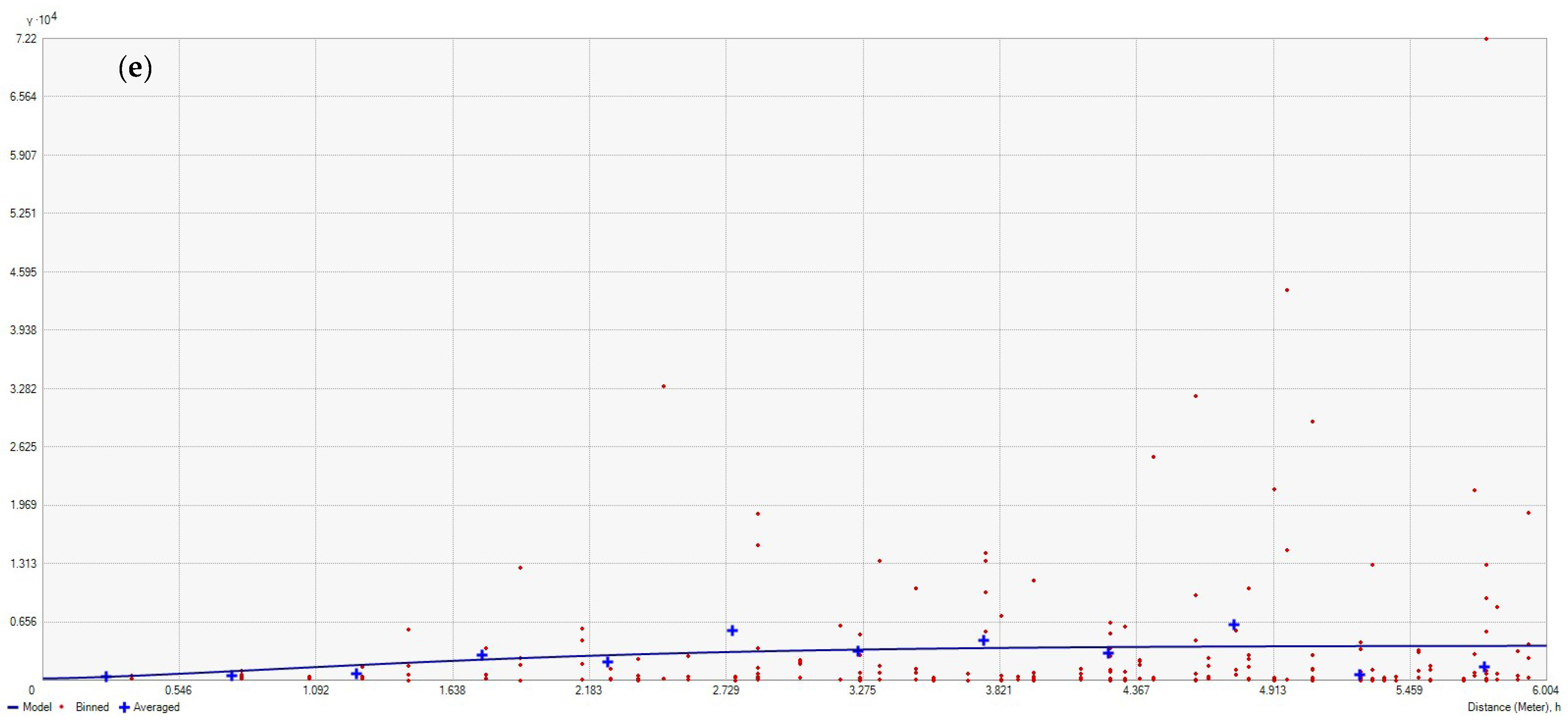
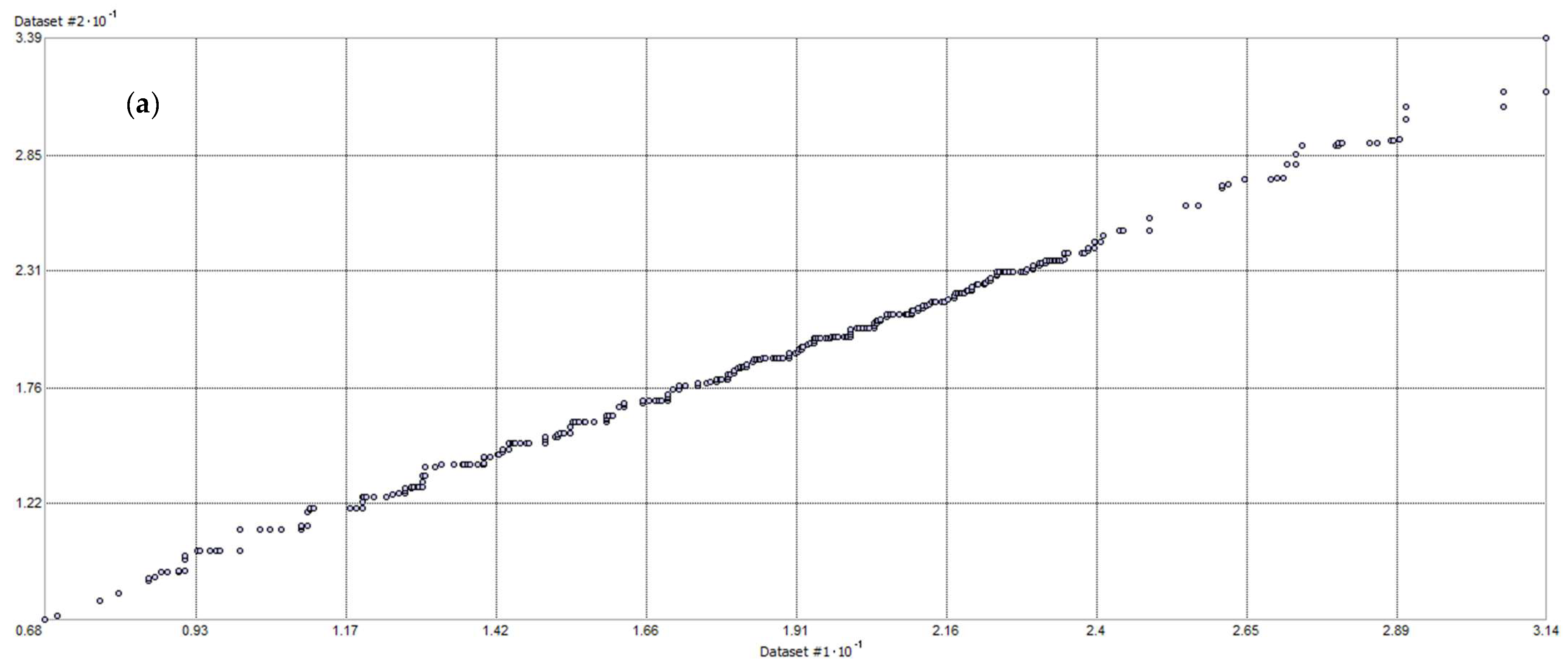
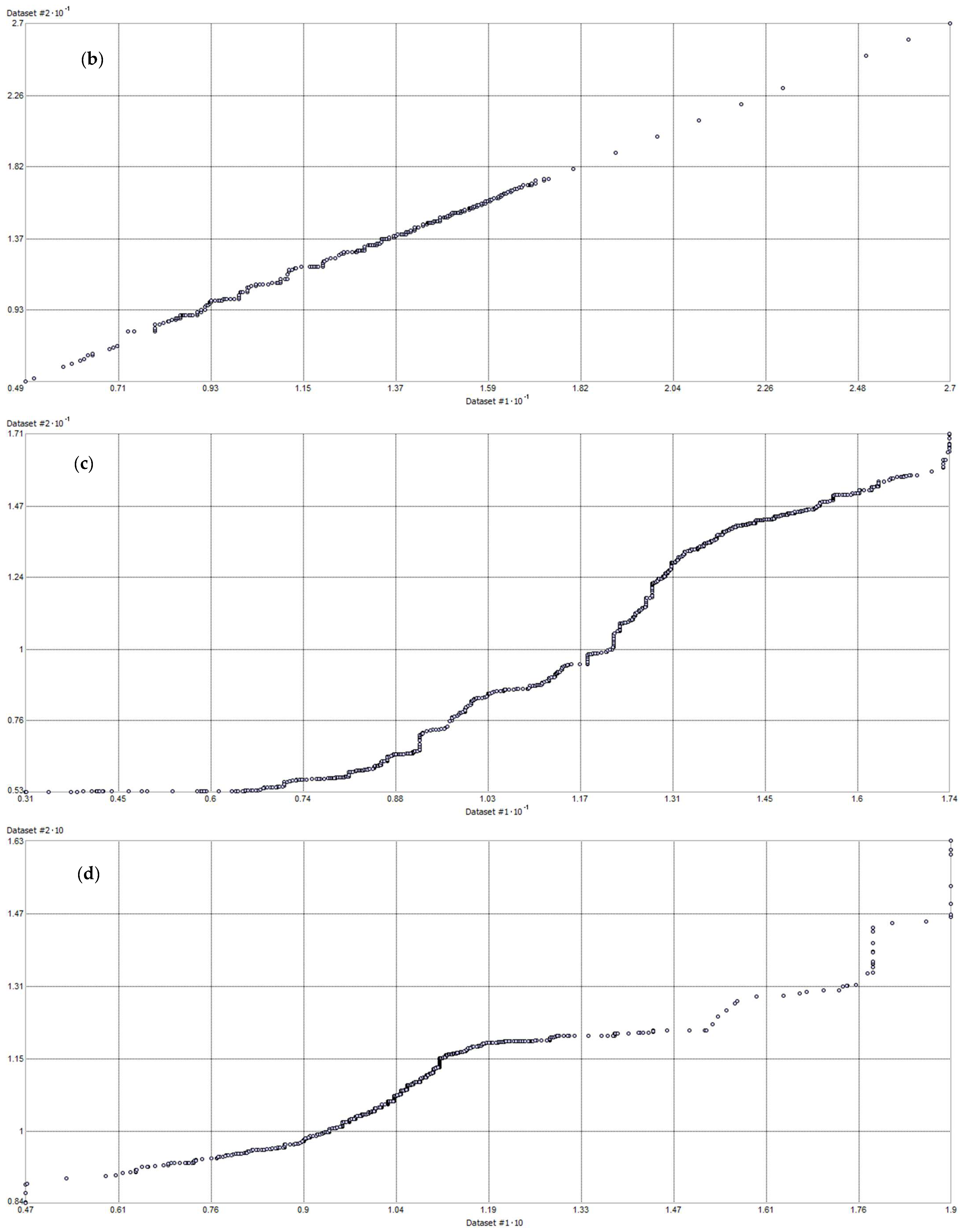
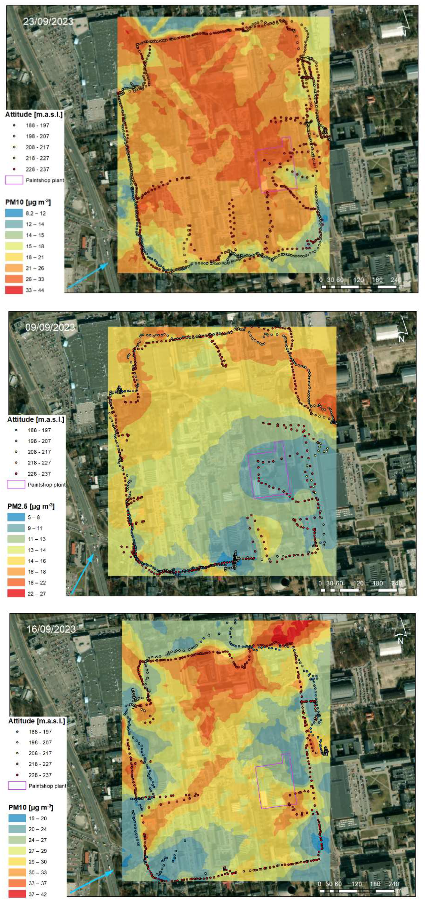
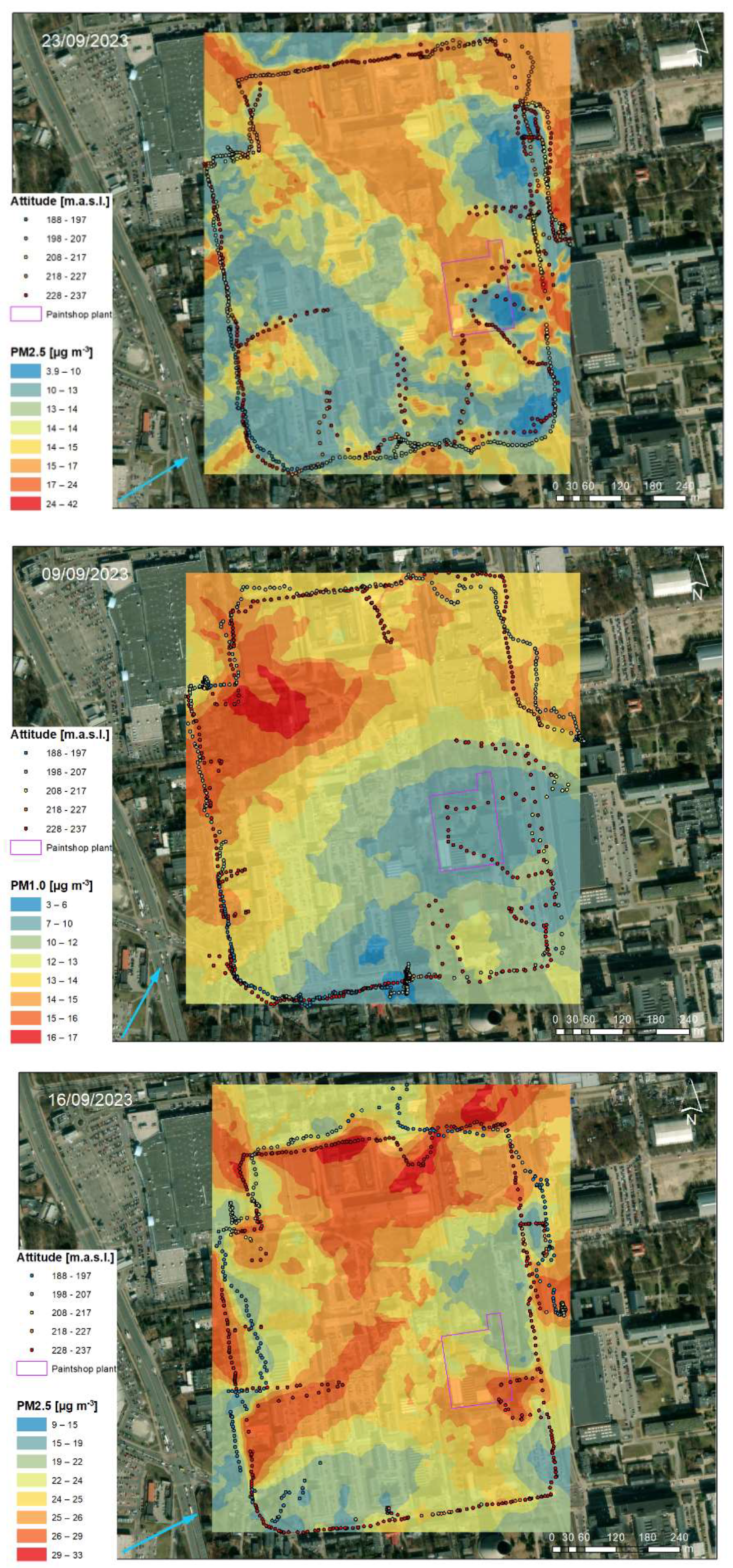
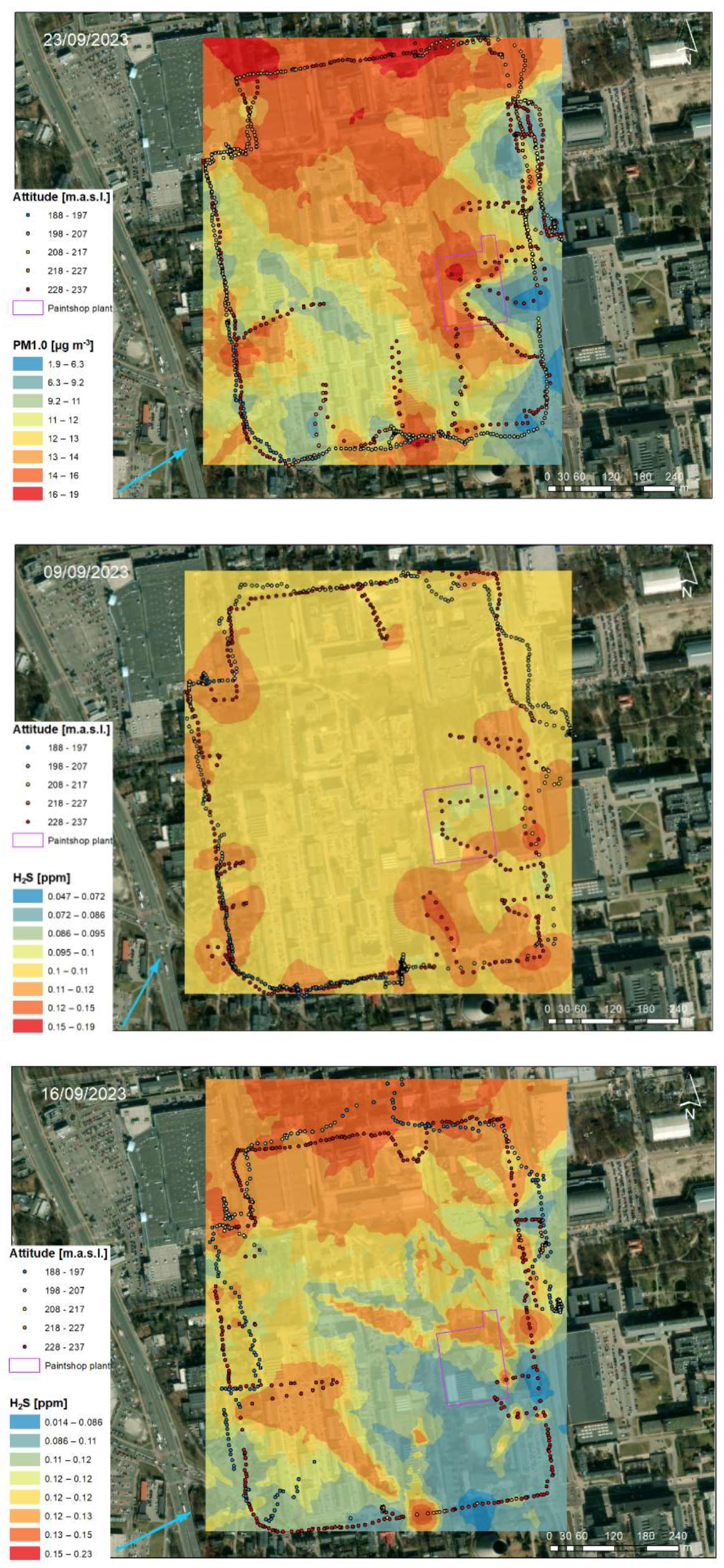
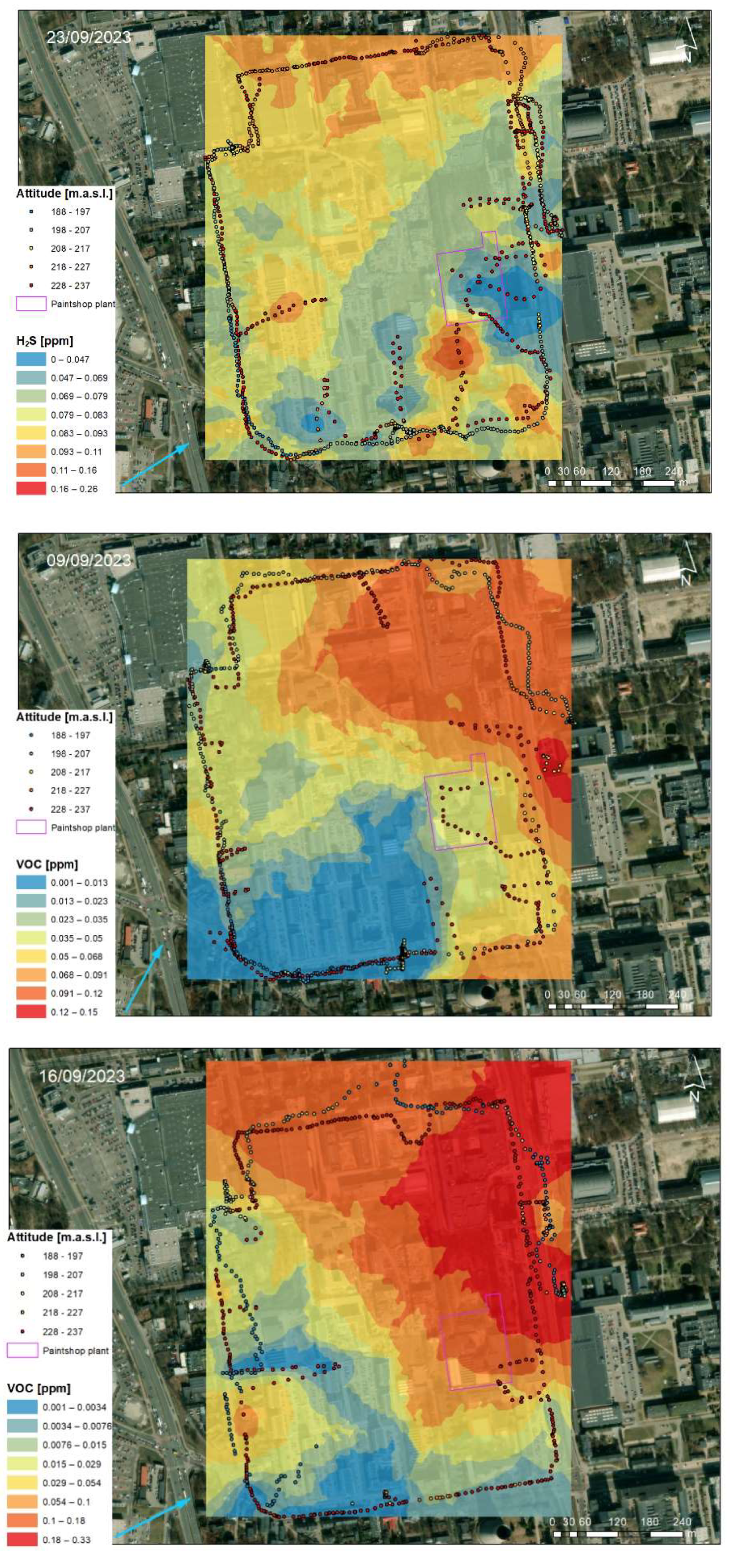
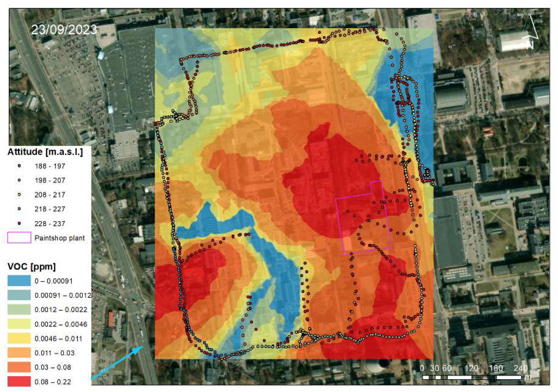
3.2. Geostatistical Analysis of Atmospheric Pollution Concentrations

In this study, the results of in situ measurements of atmospheric pollution levels in the vicinity of the paintshop were represented as the data interpretation and visualization of related time series based on GIS tools. The interpolated surfaces of the spatial distribution of air pollutants for each sampling campaign obtained for the kriging interpolation technique are shown in Figure 6. The ordinary kriging predictions produced a realistic estimation of pollutant levels over the study area. The interpolation results showed a short-scale variation in particulates ranging from 8 to 44 µg m−3, which was very similar to measurements made with an unmanned aerial vehicle (UAV). The predicted levels of H2S and VOC in the entire analysis area were reasonable compared to field observations, with concentrations ranging from 0.05 to 0.26 ppm and 0.01 to 0.33 ppm, respectively. A slight structural overestimation of the predicted H2S levels compared to the concentration under the UAV measurements was evident only in data from 16 and 23 September (Figure 6).
Based on the prevailing southwest wind direction, higher levels of selected pollutants resulting from the UAV survey and kriging interpolation were observed in the northern and eastern parts of the study area. A visual comparison indicated that there was no clear correlation between the levels of particulate matter pollutants and interpolated surface features near the paintshop plant in the three sampling campaigns. The interpolated map showed higher values of particulates towards the communication routes and surrounding buildings. In the case of H2S concentration distribution, it tended to decrease in the southern and middle part of the study area. Despite the large scale of spatial variability of the predicted H2S concentration for the three measurement campaigns, there were no pronounced hot spots of hydrogen sulfide in the study area (Figure 6).
The situation was completely different in the case of volatile organic compounds, as there was a space on the west side and the north side of the investigated region with a highly enhanced emission of VOCs compared to the surroundings. According to the Kriging prediction, the spatial distribution of VOCs in all measurement campaigns has a common pattern, associated with high concentrations of pollution at the shortest distance from the paintshop. The interpolation maps based on the UAV measurements revealed very similar spatial structures of VOC dispersion, with maximum pollution levels most prominent downwind of the emission source. The increased levels of VOC in the air were recorded at heights of 30–40 m a.g.l., where the paintshop stacks are located, which confirms that the pollutants are of industrial origin.
In general, the maps of spatially distributed pollution showed a good correlation between air pollution concentrations measured in vertical profiles compared to interpolated surfaces. The relative accuracy of interpolation for atmospheric pollution concentrations produced by ordinary kriging was confirmed by the prediction errors, as long as the results of the semivariogram model had a significant spatial autocorrelation (the values of variation increased with distance) (see Figure A3). Results of predictions were also analyzed using the General Q-Q plot in the Geostatistical Analyst Tool in ArcGIS 10.8 software. The obtained values of the prediction model for PM10 and PM2.5 were within a narrow range (minor deviations) from the observed values (see Figure A4); however, in the case of PM1.0, H2S and VOC observations, the points deviated greatly from the real range, with fairly sharp corners in the tail (see Figure A4). These results were clustered along the UAV-measured transects since sampling points were densely located and not evenly distributed throughout the area.
On the other hand, when dealing with significant spatial variation and different surface features, the effects of differences in measurement height and plume position, combined with a mean vertical wind profile and detail analyses in some missing areas using more sample points, need to be assumed. Moreover, this case study and the results of spatio-temporal predictions (kriging interpolation maps) can be used in the design of parameters of further UAV measurements in complex urban environments.

4. Conclusions

There was a significant difference in the level of air pollutants throughout the altitude profiles during the three UAV survey campaigns in September 2021. However, the pollutant concentrations showed similar vertical profiles, which likely resulted from flying in the layer of the most concentrated gaseous pollutants. The measured concentrations of particulates, H2S, and VOC gradually increased with the flight altitude, reaching a minimum at the ground level and remaining nearly constant at a height of about 20 m a.g.l. The highest concentration (up to 38.5 µg m−3) of particulates (PM10, PM2.5, PM1.0) was measured at ca. 35–40 m a.g.l., whereas the lowest (ca. 10 µg m−3) was recorded at an altitude of 10–15 m a.g.l. The average values of H2S and VOC gradually increased from the surface to vertical profiles of about 30–40 m a.g.l., reaching a maximum of 0.14 ppm and 0.29 ppm, respectively.
The present work reveals the adverse impact of a small paintshop on pollution levels in the neighboring atmosphere. The patterns of air pollution peaks (above 20 m level) during the study period suggest that paintshop operations contribute significantly to the formation of VOCs in the surrounding atmosphere. The obtained results are also consistent with previous studies on the spatial distribution of air pollutants coming from industrial areas using UAV flights under different emission scenarios over the city of Łódź. The present study has several limitations. The application of UAV measurements is limited in their ability to operate during unfavorable weather conditions (wind gusts above 8 m/s, low air temperature, atmospheric precipitation, low visibility), maximum flight altitude and flight time, lifting capacity and spatial coverage. Despite certain limitations in data collection, the changes in emission levels originating from plantscale sources observed in our study indicate the role of UAV flights in determining the spatial and temporal variation of pollutants.
Integrating the UAV-obtained data with geostatistical techniques in the GIS environment made it possible to link the measured concentrations with the localized emission source. In three campaigns, the interpolated maps presented the spatial distribution of increased pollution levels of VOC at a near distance to the paintshop location. The peak VOC concentration was visible over the northeast parts of the study area located on the leeward side of the paintshop plant. The influence of this site was especially pronounced at heights of 30–40 m a.g.l. At the same time, the distributions of other measured pollutants had a different footprint compared to VOCs. During the study period, at exactly the same spatial location, the concentrations of other pollutants did not exceed the above atmospheric levels.
Cross-validation tests determined that the prediction of air pollution was of acceptable accuracy. However, although maps of pollution distribution showed similar spatial concentration structures close to the examined industrial facilities, the limited number of sampling points in the center of interpolation extent and edge effects of the clustered location of sampling points could affect the quality of the interpolated outputs. Therefore, in the future, more UAV measurement campaigns will be conducted throughout the additional sampling locations, and information on the potential impact of a small paintshop on the surrounding atmosphere will be updated with new data.

Author Contributions

Conceptualization, I.S.; methodology, I.S., R.C., M.D. and Y.B.; software, I.S., R.C., M.D. and Y.B.; validation, I.S. and Y.B.; formal analysis, I.S.; investigation, I.S., R.C., M.D. and Y.B.; data curation, Y.B. and M.D.; writing—original draft preparation, I.S., R.C., M.D. and Y.B.; writing—review and editing, I.S, R.C., M.D. and Y.B.; visualization, M.D. and Y.B.; supervision, I.S.; funding acquisition, I.S. and R.C. All authors have read and agreed to the published version of the manuscript.

Funding

This study was carried out with the financial support of the Provincial Fund for Environmental Protection and Water Management in Łódź (in Polish: Wojewódzki Fundusz Ochrony Środowiska i Gospodarki Wodnej w Łodzi) as part of the project “Spatial analysis of changes in air pollution in the Łódź agglomeration” (project number 590/BN/D/2018).

Data Availability Statement

Data are contained within the article.

Conflicts of Interest

The authors declare no conflict of interest. The funders had no role in the design of the study; in the collection, analyses, or interpretation of data; in the writing of the manuscript; or in the decision to publish the results.

Appendix A

Figure A1. The scatter plot matrix of temporal changes in pollutant distributions and their correlations with air temperature and relative humidity in vertical profiles measured in the vicinity of the paintshop during sampling campaigns in September 2021.
Energies 16 07716 g0a1aEnergies 16 07716 g0a1bEnergies 16 07716 g0a1c
Figure A2. Box plot series and pairwise comparisons (Tukey’s test) of temporal changes in pollutant concentrations, with air temperature and relative humidity in vertical profiles measured in the vicinity of the paintshop during sampling campaigns in September 2021. Different letters indicate significant differences between groups (p = 0.05).
Energies 16 07716 g0a2aEnergies 16 07716 g0a2b
Figure A3. The semivariance models of the ordinary kriging interpolation method showing the spatial correlations for (a) PM10; (b) PM2.5; (c) PM1.0; (d) H2S; (e) VOC.
Energies 16 07716 g0a3aEnergies 16 07716 g0a3bEnergies 16 07716 g0a3c
Figure A4. Q-Q Plots of sample normal quantiles (Y axis) vs. theoretical/predicted quantiles (X axis) resulting from the ordinary kriging interpolation method for (a) PM10; (b) PM2.5; (c) PM1.0; (d) H2S; (e) VOC.
Energies 16 07716 g0a4aEnergies 16 07716 g0a4bEnergies 16 07716 g0a4c

References

  1. Volatile Organic Compounds’ Impact on Indoor Air Quality. Available online: https://www.epa.gov/indoor-air-quality-iaq/volatile-organic-compounds-impact-indoor-air-quality#Sources (accessed on 18 January 2022).
  2. Wei, B.; Zhang, W.; Chao, J.; Zhang, T.; Zhao, T.; Noctor, G.; Liu, Y.; Han, Y. Functional analysis of the role of hydrogen sulfide in the regulation of dark-induced leaf senescence in Arabidopsis. Sci. Rep. 2017, 7, 2615. [Google Scholar] [CrossRef]
  3. Kourtidis, K.; Kelesis, A.; Petrakakis, M. Hydrogen sulfide (H2S) in urban ambient air. Atmos. Environ. 2008, 42, 7476–7482. [Google Scholar] [CrossRef]
  4. WHO. WHO Global Air Quality Guidelines: Paarticulate Matter (PM2.5 and PM10), Ozone, Nitrogen Dioxide, Sulfur Dioxide and Carbon Monoxide; WHO: Geneva, Switzerland, 2021. [Google Scholar]
  5. Recommendation from the Scientific Committee on Occupational Exposure Limits for Hydrogen Sulphide. 2007. Available online: https://ec.europa.eu/social/search.jsp?advSearchKey=hydrogen+sulphide&mode=advancedSubmit&langId=en (accessed on 4 September 2023).
  6. The European Parliament. European Council: On Ambient Air Quality and Cleaner Air for Europe 2008/50/EC. Available online: https://www.eumonitor.eu/9353000/1/j9vvik7m1c3gyxp/vhvvygrp44xc (accessed on 4 September 2023).
  7. Atkinson, R.W.; Mills, I.C.; Walton, H.A.; Anderson, H.R. Fine particle components and health—A systematic review and meta-analysis of epidemiological time series studies of daily mortality and hospital admissions. J. Expo. Sci. Environ. Epidemiol. 2015, 25, 208–214. [Google Scholar] [CrossRef] [PubMed]
  8. Bougiatioti, A.; Kanakidou, M.; Mihalopoulos, N. Air Quality in European Cities. In Comprehensive Analytical Chemistry; Elsevier: Amsterdam, The Netherlands, 2016; pp. 517–542. [Google Scholar]
  9. Jońca, J.; Pawnuk, M.; Bezyk, Y.; Arsen, A.; Sówka, I. Drone-Assisted Monitoring of Atmospheric Pollution—A Comprehensive Review. Sustainability 2022, 14, 11516. [Google Scholar] [CrossRef]
  10. Cichowicz, R.; Dobrzański, M. 3D Spatial Analysis of Particulate Matter (PM10, PM2.5 and PM1.0) and Gaseous Pollutants (H2S, SO2 and VOC) in Urban Areas Surrounding a Large Heat and Power Plant. Energies 2021, 14, 4070. [Google Scholar] [CrossRef]
  11. Lambey, V.; Prasad, A.D. A Review on Air Quality Measurement Using an Unmanned Aerial Vehicle. Water Air Soil Pollut. 2021, 232, 109. [Google Scholar] [CrossRef]
  12. Li, C.; Liu, M.; Hu, Y.; Wang, H.; Xiong, Z.; Wu, W.; Liu, C.; Zhang, C.; Du, Y. Investigating the vertical distribution patterns of urban air pollution based on unmanned aerial vehicle gradient monitoring. Sustain. Cities Soc. 2022, 86, 104144. [Google Scholar] [CrossRef]
  13. Motlagh, N.H.; Irjala, M.; Zuniga, A.; Lagerspetz, E.; Rantala, V.; Flores, H.; Nurmi, P.; Tarkoma, S. Toward Blue Skies: City-Scale Air Pollution Monitoring Using UAVs. IEEE Consum. Electron. Mag. 2023, 12, 21–31. [Google Scholar] [CrossRef]
  14. Guin, M.K.; Hiremath, S.; Shrishail, M.H. Semi-Autonomous UAV based Weather and Air Pollution Monitoring System. J. Phys. Conf. Ser. 2021, 1921, 012091. [Google Scholar] [CrossRef]
  15. Van den Bossche, J.; Peters, J.; Verwaeren, J.; Botteldooren, D.; Theunis, J.; De Baets, B. Mobile monitoring for mapping spatial variation in urban air quality: Development and validation of a methodology based on an extensive dataset. Atmos. Environ. 2015, 105, 148–161. [Google Scholar] [CrossRef]
  16. Wang, S.; Ma, Y.; Wang, Z.; Wang, L.; Chi, X.; Ding, A.; Yao, M.; Li, Y.; Li, Q.; Wu, M.; et al. Mobile monitoring of urban air quality at high spatial resolution by low-cost sensors: Impacts of COVID-19 pandemic lockdown. Atmos. Chem. Phys. 2021, 21, 7199–7215. [Google Scholar] [CrossRef]
  17. Schilt, U.; Barahona, B.; Buck, R.; Meyer, P.; Kappani, P.; Möckli, Y.; Meyer, M.; Schuetz, P. Low-Cost Sensor Node for Air Quality Monitoring: Field Tests and Validation of Particulate Matter Measurements. Sensors 2023, 23, 794. [Google Scholar] [CrossRef] [PubMed]
  18. Samad, A.; Alvarez Florez, D.; Chourdakis, I.; Vogt, U. Concept of Using an Unmanned Aerial Vehicle (UAV) for 3D Investigation of Air Quality in the Atmosphere—Example of Measurements Near a Roadside. Atmosphere 2022, 13, 663. [Google Scholar] [CrossRef]
  19. Jumaah, H.J.; Kalantar, B.; Halin, A.A.; Mansor, S.; Ueda, N.; Jumaah, S.J. Development of UAV-Based PM2.5 Monitoring System. Drones 2021, 5, 60. [Google Scholar] [CrossRef]
  20. Cichowicz, R.; Dobrzański, M. Spatial Analysis (Measurements at Heights of 10 m and 20 m above Ground Level) of the Concentrations of Particulate Matter (PM10, PM2.5, and PM1.0) and Gaseous Pollutants (H2S) on the University Campus: A Case Study. Atmosphere 2021, 12, 62. [Google Scholar] [CrossRef]
  21. Pochwała, S.; Anweiler, S.; Deptuła, A.; Gardecki, A.; Lewandowski, P.; Przysiężniuk, D. Optimization of air pollution measurements with unmanned aerial vehicle low-cost sensor based on an inductive knowledge management method. Optim. Eng. 2021, 22, 1783–1805. [Google Scholar] [CrossRef]
  22. Rohi, G.; Ejofodomi, O.; Ofualagba, G. Autonomous monitoring, analysis, and countering of air pollution using environmental drones. Heliyon 2020, 6, e03252. [Google Scholar] [CrossRef] [PubMed]
  23. Babak, V.P.; Babak, S.V.; Eremenko, V.S.; Kuts, Y.V.; Myslovych, M.V.; Scherbak, L.M.; Zaporozhets, A.O. Monitoring the Air Pollution with UAVs. In Models and Measures in Measurements and Monitoring; Springer: Berlin/Heidelberg, Germany, 2021; pp. 191–225. [Google Scholar]
  24. Brander, L.M.; Bräuer, I.; Gerdes, H.; Ghermandi, A.; Kuik, O.; Markandya, A.; Navrud, S.; Nunes, P.A.L.D.; Schaafsma, M.; Vos, H.; et al. Using Meta-Analysis and GIS for Value Transfer and Scaling Up: Valuing Climate Change Induced Losses of European Wetlands. Environ. Resour. Econ. 2012, 52, 395–413. [Google Scholar] [CrossRef]
  25. Nichol, J.E.; Wong, M.S.; Wang, J. A 3D aerosol and visibility information system for urban areas using remote sensing and GIS. Atmos. Environ. 2010, 44, 2501–2506. [Google Scholar] [CrossRef]
  26. Vizcaino, P.; Pistocchi, A. Use of a Simple GIS-Based Model in Mapping the Atmospheric Concentration of γ-HCH in Europe. Atmosphere 2014, 5, 720–736. [Google Scholar] [CrossRef]
  27. Bezyk, Y.; Sówka, I.; Górka, M.; Blachowski, J. GIS-Based Approach to Spatio-Temporal Interpolation of Atmospheric CO2 Concentrations in Limited Monitoring Dataset. Atmosphere 2021, 12, 384. [Google Scholar] [CrossRef]
  28. Li, J.; Heap, A.D. Spatial interpolation methods applied in the environmental sciences: A review. Environ. Model. Softw. 2014, 53, 173–189. [Google Scholar] [CrossRef]
  29. Li, L.; Zhou, X.; Kalo, M.; Piltner, R. Spatiotemporal Interpolation Methods for the Application of Estimating Population Exposure to Fine Particulate Matter in the Contiguous U.S. A Real-Time Web Application. Int. J. Environ. Res. Public Health 2016, 13, 749. [Google Scholar] [CrossRef] [PubMed]
  30. Matejicek, L. Spatial modelling of air pollution in urban areas with GIS: A case study on integrated database development. Adv. Geosci. 2005, 4, 63–68. [Google Scholar] [CrossRef]
  31. Ristanović, B.; Cimbaljević, M.; Miljković, Đ.; Ostojić, M.; Fekete, R. GIS Application for Determining Geographical Factors on Intensity of Erosion in Serbian River Basins. Case Study: The River Basin of Likodra. Atmosphere 2019, 10, 526. [Google Scholar] [CrossRef]
  32. Super, I.; Dellaert, S.N.C.; Visschedijk, A.J.H.; Denier van der Gon, H.A.C. Uncertainty analysis of a European high-resolution emission inventory of CO2 and CO to support inverse modelling and network design. Atmos. Chem. Phys. 2020, 20, 1795–1816. [Google Scholar] [CrossRef]
  33. Li, Z. An enhanced dual IDW method for high-quality geospatial interpolation. Sci. Rep. 2021, 11, 9903. [Google Scholar] [CrossRef]
  34. De Jesus, K.L.M.; Senoro, D.B.; Dela Cruz, J.C.; Chan, E.B. A Hybrid Neural Network–Particle Swarm Optimization Informed Spatial Interpolation Technique for Groundwater Quality Mapping in a Small Island Province of the Philippines. Toxics 2021, 9, 273. [Google Scholar] [CrossRef]
  35. Jiang, B.; Xu, W.; Zhang, D.; Nie, F.; Sun, Q. Contrasting multiple deterministic interpolation responses to different spatial scale in prediction soil organic carbon: A case study in Mollisols regions. Ecol. Indic. 2022, 134, 108472. [Google Scholar] [CrossRef]
  36. Population. Statistical Office in Lodz. Available online: https://lodz.stat.gov.pl/ (accessed on 16 January 2022).
  37. City of Lodz. Statistical Office in Lodz. Available online: https://lodz.stat.gov.pl/vademecum/vademecum_lodzkie/portrety_miast/miasto_lodz.pdf (accessed on 16 January 2022).
  38. Chief Inspectorate for Environmental Protection. Annual Assessment of Air Quality in the Łódź Voivodeship. Provincial Report for 2021. Available online: https://powietrze.gios.gov.pl/pjp/rwms/publications/card/1684?lang=en (accessed on 11 August 2022).
  39. OpenStreetMap. Available online: https://www.openstreetmap.org (accessed on 11 November 2020).
  40. Climate in Lódz, Poland. Available online: https://weather-and-climate.com/average-monthly-Rainfall-Temperature-Sunshine,lodz,Poland (accessed on 16 January 2022).
  41. Climate-Data.org. Available online: https://en.climate-data.org/europe/poland/lower-silesian-voivodeship-456/ (accessed on 9 October 2021).
  42. Weather Atlas. Monthly Weather Forecast and Climate Łódź, Poland. Available online: https://www.weather-atlas.com/en/poland/lodz-climate#uv_index (accessed on 16 January 2022).
  43. Climate and Average Weather Year Round at Lodz Lublinek Poland. Available online: https://weatherspark.com/y/150026/Average-Weather-at-Lodz-Lublinek-Poland-Year-Round (accessed on 16 January 2022).
  44. Meteorological Data. IMGW. Available online: https://danepubliczne.imgw.pl/data/dane_pomiarowo_obserwacyjne/dane_meteorologiczne/miesieczne/synop/2021/ (accessed on 16 January 2022).
  45. Cichowicz, R.; Dobrzański, M. Indoor and Outdoor Concentrations of Particulate Matter (PM10, PM2.5) and Gaseous Pollutants (VOC, H2S) on Different Floors of a University Building: A Case Study. J. Ecol. Eng. 2021, 22, 162–173. [Google Scholar] [CrossRef]
  46. Sówka, I.; Cichowicz, R.; Dobrzański, M.; Bezyk, Y. Application of mobile platform and geostatistical methods in the analysis of air quality in the selected area of the city of Lodz. In Proceedings of the 4th Symposium “Air Quality and Health”, Wrocław, Poland, 3–5 July 2023; Korzystka-Muskała, M., Kubicka, J., Sawiński, T., Drzeniecka-Osiadacz, A., Eds.; University of Wrocław: Wrocław, Poland, 2023; pp. 94–95. [Google Scholar]
Figure 1. Location of the study site (19°26′46.681″ E 51°44′50.879″ N) in the city of Łódź. Area is divided into several smaller building elements (own study, based on background source). Base map source [39].
Energies 16 07716 g001
Figure 2. Wind speed data for the city of Łódź in 2021 (own study based on data from source [44]).
Energies 16 07716 g002
Figure 3. Measurement and sampling apparatus installed on (A) an unmanned aerial vehicle (UAV); (B) a mobile, ground-based platform (GP).
Energies 16 07716 g003
Figure 4. Temporal changes in pollutant concentration and air temperature in vertical profiles measured in the vicinity of the paintshop during sampling campaigns in September 2021.
Energies 16 07716 g004aEnergies 16 07716 g004b
Figure 5. Vertical profiles of pollutant concentrations (PM10, PM2.5, PM1.0, H2S, VOC) measured in the vicinity of the paintshop during sampling campaigns in September 2021. Bullets represent sampling data.
Energies 16 07716 g005
Figure 6. Spatial changes in pollutants concentrations in vertical profiles in the vicinity of the paintshop during sampling campaigns in September 2021, using the ordinary kriging interpolation method. The arrows indicate dominant wind direction.
Energies 16 07716 g006aEnergies 16 07716 g006bEnergies 16 07716 g006cEnergies 16 07716 g006dEnergies 16 07716 g006eEnergies 16 07716 g006f
Table 1. Design features for buildings surrounding the paintshop site in the immediate vicinity.
Location in
Relation to the Paintshop
Distance to the Paintshop [m]Building FeatureDescription
North200–300 Residential, multi-family, and commercial buildingsDominated height of 15–30 m
South100–200Residential, multifamily buildingsDominated height of 15–30 m
West100–200Single-family buildings and service facilitiesDominated height of 6–15 m
East100–300Facilities at the Łódź University of Technology and academic estateDominated height of 27–33 m
Table 2. Weather conditions during sampling campaigns measured in the vicinity of the paintshop.
CampaignsAir Temperature [°C]Real Humidity [%]Air Pressure [hPa]Wind Speed [m·s–1]Wind Direction [°]
9 September 2021
Min.21.336.01018.22.0176
Max.24.355.01019.44.0197
Avg.23.144.01018.93.3191
St. Dev.1.38.00.61.010
16 September 2021
Min.20.070.01011.33.0212
Max.23.382.01011.94.0254
Avg.21.877.01011.73.5232
St. Dev.1.45.10.30.617
23 September 2021
Min.13.281.01014.34.0228
Max.14.988.01017.46.0248
Avg.14.383.01015.95.25237
St. Dev.0.83.41.41.08
Disclaimer/Publisher’s Note: The statements, opinions and data contained in all publications are solely those of the individual author(s) and contributor(s) and not of MDPI and/or the editor(s). MDPI and/or the editor(s) disclaim responsibility for any injury to people or property resulting from any ideas, methods, instructions or products referred to in the content.

