Article

A Deep Neural Network-Based Optimal Scheduling Decision-Making Method for Microgrids

1
China Southern Power Grid Guizhou Power Grid Co., Ltd., Guiyang 550003, China
2
School of Electrical Engineering, Guizhou University, Guiyang 550025, China
*
Author to whom correspondence should be addressed.
Energies 2023, 16(22), 7635; https://doi.org/10.3390/en16227635
Submission received: 13 October 2023 / Revised: 13 November 2023 / Accepted: 16 November 2023 / Published: 17 November 2023

Abstract

:
With the rapid growth in the proportion of renewable energy access and the structural complexity of distributed energy systems, traditional microgrid (MG) scheduling methods that rely on mathematical optimization models and expert experience are facing significant challenges. Therefore, it is essential to present a novel scheduling technique with high intelligence and fast decision-making capacity to realize MGs’ automatic operation and regulation. This paper proposes an optimal scheduling decision-making method for MGs based on deep neural networks (DNN). Firstly, a typical mathematical scheduling model used for MG operation is introduced, and the limitations of current methods are analyzed. Then, a two-stage optimal scheduling framework comprising day-ahead and intra-day stages is presented. The day-ahead part is solved by mixed integer linear programming (MILP), and the intra-day part uses a convolutional neural network (CNN)—bidirectional long short-term memory (Bi LSTM) for high-speed rolling decision making, with the outputs adjusted by a power correction balance algorithm. Finally, the validity of the model and algorithm of this paper are verified by arithmetic case analysis.

1. Introduction

MGs, characterized by cleanliness, low-carbon emissions, and openness, have garnered significant attention due to the rapid development of renewable energy in recent years [1]. As a critical solution to improve the consumption of distributed power sources and the reliability of power supply, MGs have become essential to reducing fossil energy pollution and promoting sustainable development in China [2]. However, the intermittent, volatile, and uncertain nature of renewable energy sources poses significant challenges to the stable operation of MGs [3]. Additionally, the expansion of the MG system and the increased number of its components also impose more demanding requirements on the optimal scheduling method. The traditional scheduling method based on numerical model optimization, scenario matching, and manual manning makes it difficult to meet the demand. Hence, studying fast, accurate, and intelligent scheduling decision methods holds immense practical value and significance [4].
Currently, the predominant method for solving MG optimal scheduling problems is a numerical calculation method grounded in optimization theory. Common optimal scheduling models encompass MILP [5], dynamic programming [6], distributed optimization [7], etc. Likewise, common model-solving algorithms involve intelligent algorithms [8], second-order cone relaxation methods [9], Lagrange relaxation methods, etc. However, as the uncertainties of the source–load dual-side within MGs escalate, solving the optimal scheduling problem under such uncertainties becomes a more realistic and challenging research problem [10]. Some researchers construct uncertainty planning models. The main modeling and solution methods are stochastic planning [11], chance-constrained planning [12], etc. Among these, robust optimization [13,14] methods have been proven to be an effective method of solving MG uncertain optimization problems. They aim at optimal operation under the worst-case scenario. However, their overly pessimistic view of uncertain variables may lead to solution results that are too conservative to be economical. The mathematical models of these methods are relatively complex and computationally expensive. The other researchers used a multi-timescale optimal scheduling strategy [15], which can be classified into day-ahead scheduling and intra-day stage according to the timescale. Among these, the model predictive control (MPC) technique is a widely employed modeling approach [16]. How to enhance intra-day real-time scheduling computational efficiency is still a challenge.
In summary, the traditional optimization theory-based scheduling methods rely on strict mathematical derivation, requiring researchers to participate. With the MG evolving into a new system characterized by increased uncertainty and complexity, the traditional optimization scheduling methods are gradually becoming inadequate to meet the demands of MG operation [17]. Several critical problems of this method are as follows:
(1)
The traditional mathematical optimization methods cannot model the components of the MG in a fast and refined manner, but it is difficult to describe the physical characteristics of the actual operation of the components using a simplified model [18].
(2)
The traditional mathematical MG scheduling models are often nonlinear and nonconvex, which is a typical nondeterministic polynomial problem (NP-hard). The problem is demanding on the solution algorithm, and it is not easy to find the optimal solution.
(3)
The computational process of traditional mathematical optimization methods is complex and inefficient, and it is difficult to adapt to the real-time solution of optimization scheduling problems with uncertainty under complex and variable system operating conditions [19].
(4)
The traditional mathematical optimization methods ignore the significance of historical data and historical decision-making plans and fail to make use of the valuable historical decision-making data information accumulated during the system’s operation.
Recently, the rapid development of computer technology has made neural networks (NN) an important driver of the new technological revolution and industrial change [20]. A new intelligent decision-making method using NNs based on big data technology may be a more effective way of thinking, which may help to break through the limitations of mathematical optimization solution methods. Unlike traditional optimization methods, the decision-making method based on NNs no longer depends on specific mathematical models or algorithms; instead, it is trained using extensive real data [21]. This method can greatly simplify the process and complexity of modeling and solving the optimal scheduling problem, and cope with various theoretical problems and challenges that keep emerging through its self-learning and self-evolution process. It can potentially facilitate the transition from manual supervision to machine intelligence-based monitoring in the domain of MG scheduling. Moreover, when the data make centralized training of models bitter due to factors such as privacy and size, the idea of distributed frameworks [22,23] can also be referred to for decentralized training of small models and then aggregated to a big model. This allows great flexibility in the implementation of the method. 
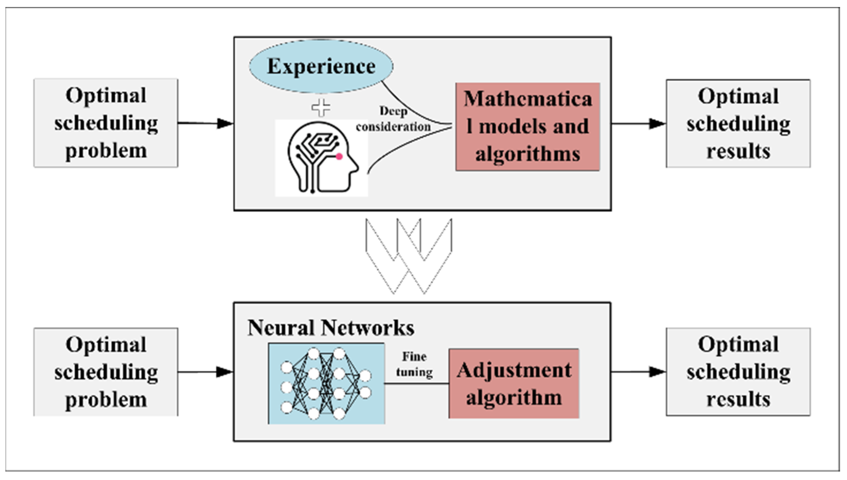
Figure 1 shows the transition from the traditional optimization method to the NN-based method.
Several scholars have attempted to utilize artificial intelligence (AI) techniques in the field of scheduling decisions. The literature [24] utilized long and short-term memory (LSTM) to establish the mapping from system load to unit output. However, the constructed network structure is relatively simple, and the results are unconstrained. The literature [25] uses a multi-layer perceptron (MLP) to learn and mimic the scheduling decision of a smart grid, and an iterative algorithm is used to correct the output of the NNs so that it satisfies the actual constraints. The literature [26] applies a feedforward neural network (FNN) for the optimal scheduling of combined heat and power (CHP) systems, which enhances computational efficiency by about 7000 times while permitting suboptimal cost. Although previous studies have demonstrated that NNs are feasible and effective in optimal energy scheduling, the current research still faces some issues:
(1)
Only load data are used as training inputs without considering the influence of other system state data on the scheduling decision results. This approach cannot fully extract the feature information embedded in the valuable historical operation data.
(2)
Only using a shallow or single network model to build the scheduling mapping relationship, the accuracy of the output results is low.
(3)
The decision results from the NNs-based scheduling method will inevitably violate some actual constraints, and there is no reasonable and efficient solution to this issue.
To address the above issues, this paper proposes a two-stage optimal scheduling method for MGs. The proposed method aims to enhance the effectiveness of the NNs-driven scheduling method and the MG’s ability to handle uncertain fluctuations and address the limitations of the traditional mathematical model-driven and manual participation scheduling methods. In the day-ahead part (1 h timescale), which does not require high timeliness, a MILP model is used to obtain the MG’s operating plan. In the day-ahead part (15 min timescale), a DNN scheduling decision network is used for fast-rolling optimization. The main contributions of this paper are as follows:
(1)
An intra-day rolling optimization model based on DNNs and big data is proposed, which is trained using the dataset clustered by the K-means algorithm to improve generalizability and accuracy.
(2)
A novel CNN-Bi LSTM scheduling decision network is proposed, digging deep feature information in the system operation data by CNN and establishing the accurate mapping between input and output by Bi LSTM.
(3)
A power balance correction algorithm is proposed to fine-tune the DNN outputs to quickly satisfy all practical constraints.
The proposed method can effectively reduce the complexity of solving the optimal scheduling problem and significantly improve computational efficiency (reducing the solution time for intra-day rolling optimization to milliseconds), which also improves the intelligence level of MGs. The rest of this paper is organized as follows: Section 2 presents the basic mathematical optimization model for day-ahead MG scheduling. Section 3 presents the DNN-based intra-day rolling optimal scheduling method. Section 4 presents simulation experiments and analyses. Section 5 presents the conclusions of this paper.

2. Microgrid Day-Ahead Optimal Scheduling Model

2.1. Overall Composition Structure of Microgrid

The specific composition structure of the MG studied in this paper is shown in Figure 2, where the arrow indicates the direction of power flow.
This MG consists of photovoltaic panels (PVs), wind turbines (WTs), microturbine (MT), upper grid (UG), storage battery (SB), and power load. The power bus is the carrier of all device power interactions. The power distribution of the entire MG is set by the scheduling center and sent to each controllable device.

2.2. Objective Function

The objective of the MG’s day-ahead optimal scheduling is to minimize the total daily operating cost. The total operating cost of the system comprises the operating and start-up costs of MT, as well as the charging/discharging costs of SB and the purchase/sale cost of UG. The above can be expressed as:
Min t = 1 T i = 1 N ( C MT , i , t + U MT , i , t ) + t = 1 T ( C SB , t + C UG , t )
C MT , i , t = a i P MT , i , t 2 + b i P MT , i , t + c i u on , i , t U MT , i , t = C U i u su , i , t C SB , t = C S SB P SB , t C UG , t = P UG , t e t
where C MT , i , t , C SB , t , and C UG , t are the operating cost of MT, SB, and UG at time t , respectively. U MT , i , t is the start-up cost of i th MT at time t . Equation (2) is a detailed expression of the cost of each device, where a i , b i , and c i are the cost factors of i th MT, and C U i is the start-up cost of i th MT. C S SB and e t are the cost factors of SB and the electricity price of UG at time t . P MT , i , t , P SB , t , and P UG , t are the power of i th MT, SB, and UG at time t , respectively. u on , i , t and u su , i , t are the binary variables for i th MT operating and starting states at time t , respectively.
The quadratic cost function of MT is linearly approximated by dividing it into S-segmented linear functions using segmented linearization methods [27], which reduces the complexity of solving the overall model. The linearization results are as follows:
C ˜ MT , i , t = c i u on , i , t + s = 1 S a s P MT , i , t , s
a s = C M T , i , s + 1 C M T , i , s P MT , i , s + 1 P MT , i , s
where C ˜ MT , i , t is the MT cost function after the linearization segments, S is the total number of segments, a s is the slope of each segment, P MT , i , s is the output of the i th MT in the s th segment.

2.3. Constraints

MG’s day-ahead optimal scheduling constraints include power balance constraint, controllable unit operation constraint, SB operation constraint, and UG operation constraint.

2.3.1. Power Balance Constraint

Equation (5) indicates that power production and consumption are balanced at all moments in the MG.
i = 1 N P MT , i , t + P SB , t + P UG , t + P WT , t + P PV , t = P Load , t , t
where P WT , t , P PV , t , and P Load , t are the power of WT, PV, and power load at time t , respectively.

2.3.2. Controllable Unit Operating Constraints

Controllable unit (MT) operating constraints include output, ramp rate, and unit status constraints. The above constraints are expressed as follows:
P MT , i min u on , i , t P MT , i , t P MT , i max , i , t
P MT , i down P MT , i , t P MT , i , t 1 P MT , i up , i , t
u su , i , t u sd , i , t = u on , i , t u on , i , t 1 , i , t
u su , i , t + u sd , i , t 1 , i , t
where P MT , i min and P MT , i max are the minimum and maximum output power of i th MT. P MT , i down and P MT , i up are the up and down ramp rate limitations of i th MT. u sd , i , t is the binary variables for i th MT stop state at time t .

2.3.3. Storage Battery Operating Constraints

SB operating constraints include charging and discharging state constraints, output power constraints, capacity constraints, and capacity cycle constraints. The above constraints are expressed as follows:
u cha , t + u dis , t 1 , t
0 P SB , t dis P max dis u dis , t , t
P max char u char , t P SB , t char 0 , t
P SB , t = η SB ( P SB , t dis u dis , t + P SB , t char u char , t ) , t
E SB , t = E SB , t 1 + P SB , t , t
E min E SB , t E max , t
E 0 = E end
where u cha , t and u dis , t are the charging and discharging binary variables at time t , respectively. P SB , t char , P SB , t dis , P max char , and P max dis are the charging and discharging power at time t and its limitation, respectively. η SB is the power conversion efficiency. E SB , t is the capacity at time t and E min , E max are the minimum and maximum capacity.

2.3.4. Power Contact Line Constraints

The constraints on UG are mainly reflected in the power transmission line which connects it to the MG. The power transmission line constraints include output constraints and purchase and sale power status constraints. The above constraints are expressed as follows:
u buy , t + u sell , t 1 , t
0 P UG , t buy P max buy u buy , t , t
P max sell u sell , t P UG , t sell 0 , t
P UG , t = P UG , t buy u buy , t + P UG , t sell u sell , t , t
where the u buy , t and u sell , t are the power purchase and sale binary variables at time t , respectively. P UG , t buy , P UG , t sell , P max buy , and P max sell are the power purchase, sale time t , and its limitation, respectively.
So far, the MG’s day-ahead optimal scheduling model based on MILP is completely constructed.

3. Deep Neural Network-Based Intra-Day Rolling Optimization Method

A data-driven DNN-based scheduling method is proposed in this paper to address the shortcomings and difficulties of traditional methods in intra-day rolling optimization. Instead of relying on specific mathematical models, it trains with large amounts of real data and makes scheduling decisions by high-dimensional matrix multiplication [28]. This method can reduce the complexity of solving the optimal scheduling problem and significantly improve computational efficiency.

3.1. Intra-Day MPC Rolling Optimization Forms

In this paper, the DNN scheduling decision network is used as an optimizer for MPC to perform intra-day rolling optimization. MPC is an alternating process of continuously rolling local optimization and continuously rolling control role implementation. By obtaining ultra-short-term power forecast information in real-time during intra-day scheduling and using the actual scheduling results and new forecast information as feedback, MPC rolling optimization forms can greatly reduce the impact of MG uncertainties on optimal operating scheduling. The general steps of MPC rolling optimization can be expressed as follows:
Step 1. Based on the current moment and the current system state, the system state in the future period is obtained by a certain prediction model.
Step 2. Based on the system state in a future period, the optimization problem in that period is solved to obtain the control sequence in that period.
Step 3. Only the action of the first moment of the control sequence is applied to the system, and the above steps are repeated for the next moment.

3.2. Total Framework of the DNN-Based Intra-Day Scheduling Decision Method

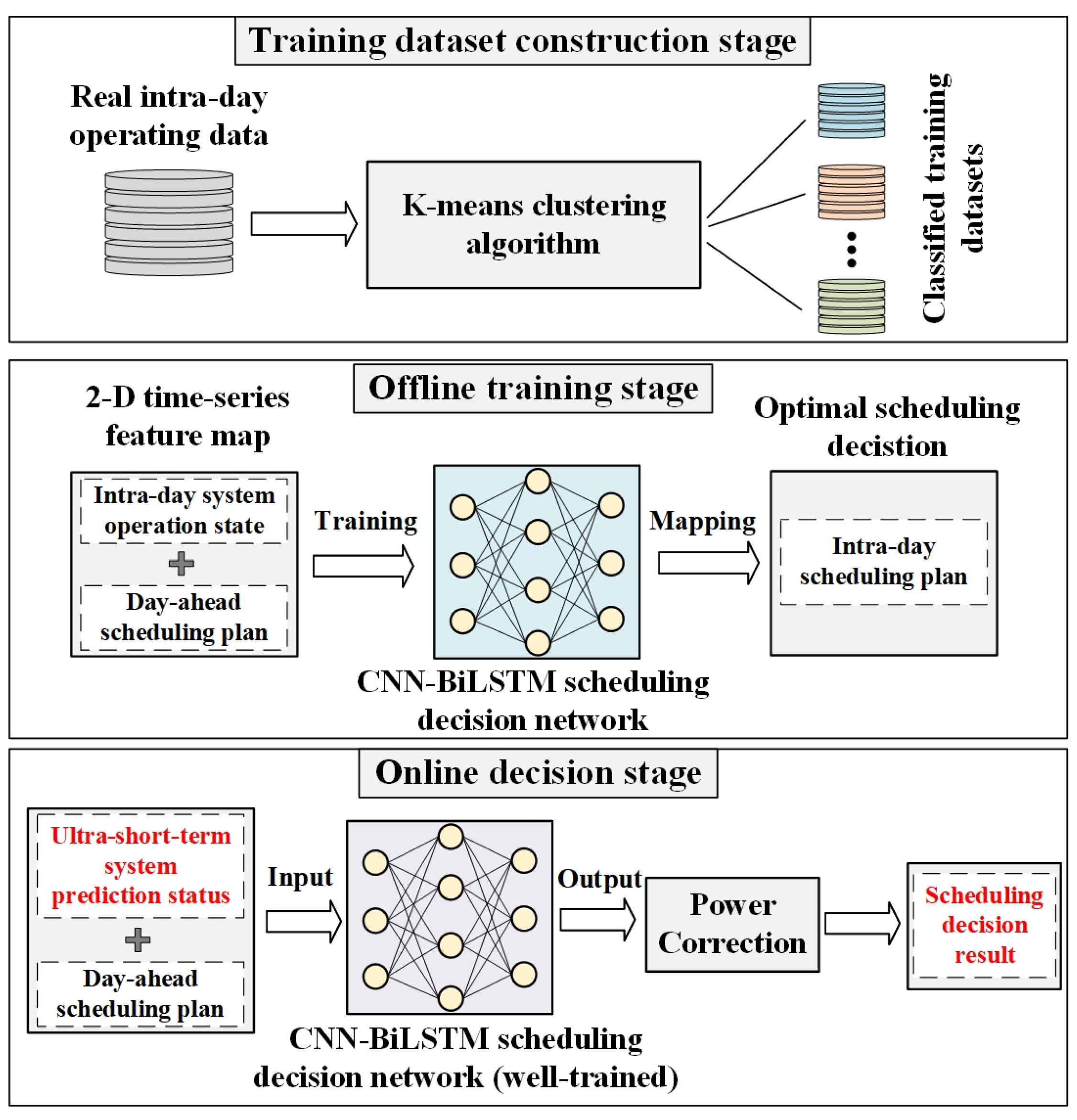
The overall framework of the DNN-based intra-day scheduling method is shown in Figure 3, which mainly includes: the training dataset construction stage, offline training stage, and online decision stage.
(1)
Training dataset construction stage. To improve the accuracy and reduce the pressure on the network’s generalizability, the numerous real operating data of MG collected are clustered by the K-means algorithm [29], dividing into different training sets. The net system load demand P Load net , which is a 96-dimensional time series represented as P Load net = P Load P Wind P PV , is used as the clustering index.
(2)
Offline training stage. A two-dimensional time series feature map containing the system operation state is constructed as the input for the CNN-Bi LSTM network. The optimal scheduling plan is the network’s output, training multiple scheduling decision networks with different training datasets.
(3)
Online decision stage. The system’s ultra-short-term prediction state is combined with the day-ahead operation plan and fed into the well-trained CNN-Bi LSTM network. The outputs of the network are fine-tuned by a power correction algorithm to get the final scheduling decision.

3.3. Introduction to Deep Neural Networks

3.3.1. Convolutional Neural Networks

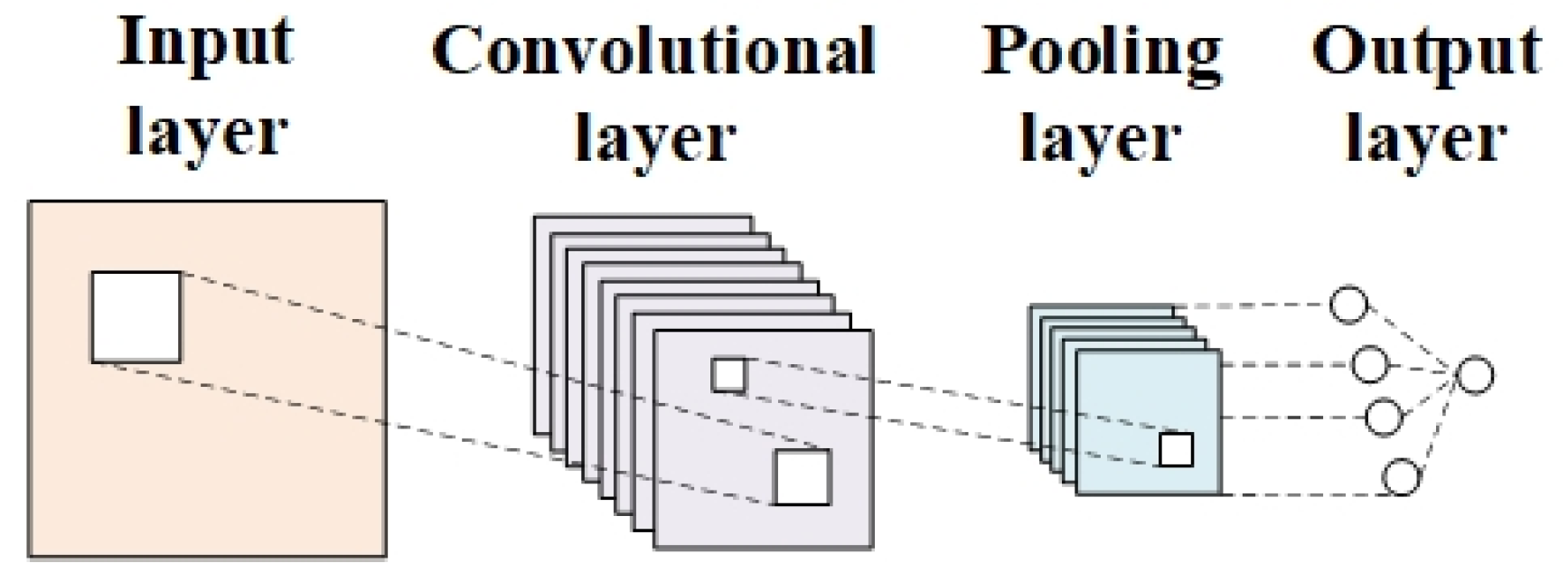
The efficient feature extraction ability of the CNN makes it the most widely used model in the field of deep learning. The CNN primarily comprises a convolutional layer and a pooling layer. The convolutional layer performs effective nonlinear local feature extraction using convolutional kernels, while the pooling layer compresses the extracted features and generates more significant feature information to enhance generalization capability [30]. The basic structure of the CNN is shown in Figure 4.

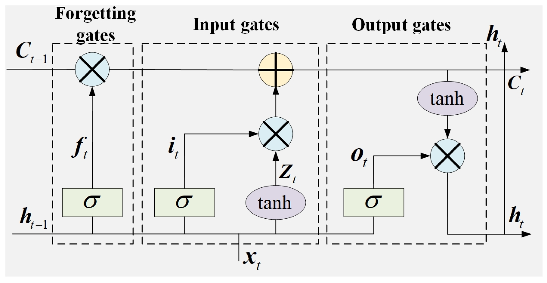
3.3.2. Bidirectional Long and Short-Term Memory Networks

We start by introducing the LSTM network, which contains forgetting gates, input gates, and output gates, and the basic structure is shown in Figure 5.
In Figure 5, σ and tanh represent Sigmoid and Tanh activation functions, respectively. The calculation of the data within LSTM is as follows:
f t = σ ( W f [ h t 1 , x t ] + b f )
i t = σ ( W i [ h t 1 , x t ] + b i )
Z t = tanh ( W c [ h t 1 , x t ] + b c )
C t = f t C t 1 + i t Z t
o t = σ ( W o [ h t 1 , x t ] + b o )
h t = o t tanh ( C t )
where W and b denote the weight matrix and bias vector, respectively. represents dot product. h t 1 and h t denote the output of the last and current moments, respectively. C t 1 and C t denote the memory state of the last and current moments, respectively. Z t is the Intermediate state of the network. i t and o t denote that the current states add degree and output degrees, respectively. x t is the input of the current moment. σ and tanh represent the sigmoid and tanh activation functions, respectively.
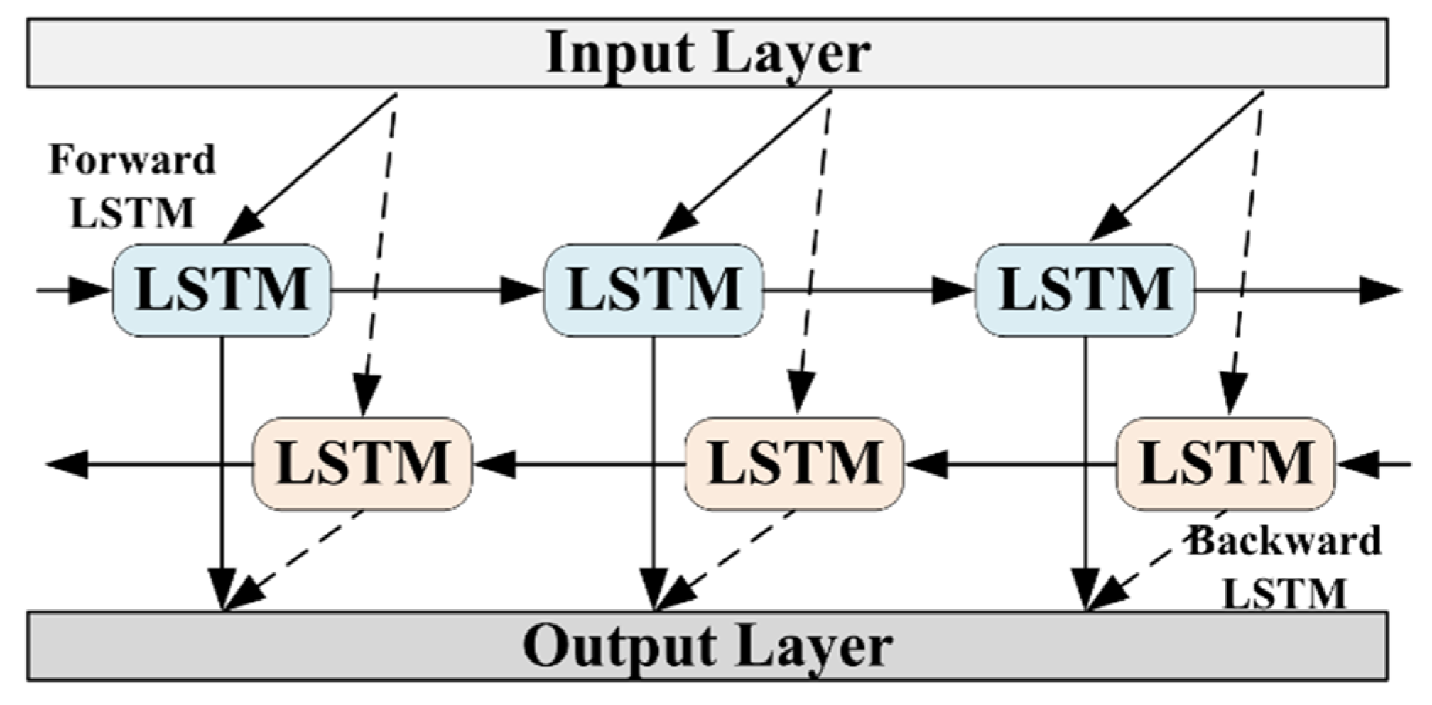
The LSTM structure gathers feature information only from the current input and past time series at each time while disregarding feature information from future time series. In this paper, bidirectional LSTM is used as the back-end mapping network of the scheduling decision network to improve the accuracy of the decision results and the performance of temporal feature extraction. The Bi LSTM is a variant structure of LSTM that includes both forward LSTM and backward LSTM layers [31]. The Bi LSTM structure enables it to gather information from both forward and backward directions, enabling the network to consider past and future data. This enhances the model’s feature extraction ability without requiring additional data. The structure of Bi LSTM is illustrated in Figure 6.

3.4. The CNN-Bi LSTM Intra-Day Scheduling Decision Network

Trained by a large amount of real operation data, the CNN-Bi LSTM intra-day scheduling decision network can learn the regularity between the system state and the scheduling decision result. Once the parameters are fixed in the network, it can provide the optimal scheduling plan extremely fast under any operating scenario.

3.4.1. Input and Output of the CNN-Bi LSTM

The CNN-Bi LSTM scheduling decision network imitates the idea of MPC for intra-day rolling optimization, with the prediction domain set to 2 h and the control domain set to 15 min. To deeply mine the implicit value information in the system operating data, we set the input X of this network in the form of a 2-D time series grayscale graph. The output Y of the network is the optimal scheduling plan. The specific expression is as follows:
X = [ P Load ( t , t + τ ) , P Wind ( t , t + τ ) , P PV ( t , t + τ ) , P SB ahead ( t , t + τ ) , P UG ahead ( t , t + τ ) , P MT ahead ( t , t + τ ) ]
Y = [ P SB * ( t , t + τ ) , P UG * ( t , t + τ ) , P MT * ( t , t + τ ) ]
X is a 9 ( τ + 1 ) matrix consisting of the intra-day state vector of the system (power load, WT, and PV) in the period t to t + τ and the day-ahead operating plan vector of controllable devices (SB, UG, and MTs) in the corresponding time. The number 9 indicates the number of input features. Y is a 1 6 ( τ + 1 ) vector consisting of the controllable devices’ intra-day optimal operating plan in the period t to t + τ . The number 6 indicates the number of controllable devices in output features. P ahead is the day-ahead operating plan, and P * is the intra-day optimal operating plan. Since the MPC prediction domain is set to 2 h, the τ is set as 7 in this paper and all the above variables are real.

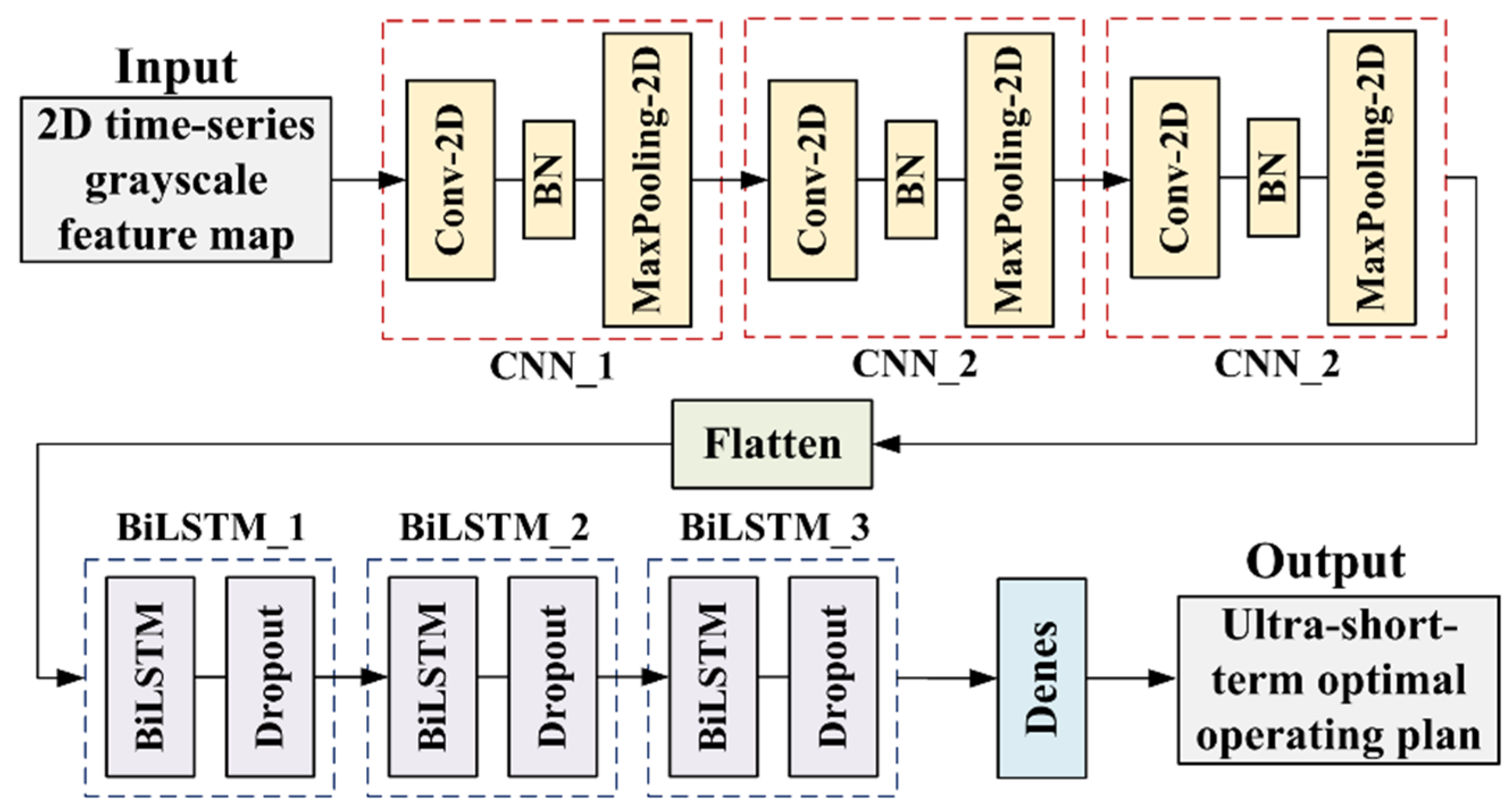
3.4.2. Structure of the CNN-Bi LSTM

Since the mapping relationship between the system operating state and scheduling decision is complex, this paper uses a multilayer CNN-Bi LSTM network for deep mining of the data. This network is mainly constituted by a three-layer CNN and a three-layer Bi LSTM, and linked by a Flatten layer. The CNN primarily extracts the power correlation feature, while the Bi LSTM focuses on extracting the power time series feature. The batch normalization (BN) layer can solve the problem of numerical instability in DNNs, making the distribution of individual features in the same batch similar. In this paper, the BN layer is inserted between each convolutional layer and pooling layer to normalize the features in the network and accelerate training. The dropout layer is the layer used after each Bi LSTM to enhance the generalization performance of the network. Finally, the data are adjusted to a vector output in the specified size through a fully connected (Dense) layer. The specific structure of the proposed CNN-Bi LSTM in this paper is shown in Figure 7.

3.4.3. Settings of the CNN-Bi LSTM

To better extract and abstract the input feature, the number of convolutional kernels is set to 64, 128, and 256, and the size of convolutional kernels is set to 7 × 7, 5 × 5, and 3 × 3. The number of neurons of Bi LSTM is set to 256, 128, and 64, respectively, and the drop rate of the dropout layer is set uniformly to 0.25.
Normalize the training data of the network to between 0 and 1 using the maximum–minimum normalization method. The network is trained using the Adam optimization algorithm [32] and the root mean square error (RMSE) is set as the loss function of the network, which is defined as follows:
RMSE = i = 1 M t = 1 T ( y i , t * y i , t ) 2 / T
where y i , t * and y i , t are the true and predicted scheduling plans for i th device at time t , respectively. M is the number of controllable devices in MG.

3.5. The Power Balance Correction Algorithm

Like load forecasting, the DNN-based scheduling method is fundamentally a process of nonlinear regression. Consequently, the output inevitably does not meet certain practical constraints. To address this issue, we use a power balance correction algorithm (PBC) to adjust the output, making it practical for use.
Inspired by the average consistency algorithm, we utilize the difference between total power demand and total generation at time t as the consistency indicator. The outputs from DNN are updated by iteration (Equations (30) and (31)). Any updated results that violate the operating constraints of the device require additional correction (Equation (32)). This algorithm is denoted as follows:
δ t [ n ] = ( P Load , t net i = 1 K P i , t [ n ] ) / K
P i , t [ n + 1 ] = P i , t [ n ] + δ t [ n ]
P i , t [ n + 1 ] = P i max , P i , t [ n + 1 ] > P i max P i min , P i , t [ n + 1 ] < P i min P i , t [ n + 1 ] + P i up , P i , t [ n + 1 ] P i , t 1 [ n + 1 ] > P i up P i , t [ n + 1 ] P i down , P i , t [ n + 1 ] P i , t 1 [ n + 1 ] < P i down P i , t [ n + 1 ] , o t h e r w i s e  
where n is the number of iterations. P i , t [ n ] and K are the power of i th power generator at time t and the total number of generators in MG, respectively.
So far, MG’s intra-day optimal scheduling model based on CNN-Bi LSTM-PBC is completely constructed.

4. Simulation Analysis and Comparison

4.1. Introduction of Example Parameters and Test System

To verify the effectiveness of the proposed method, a typical grid-connected MG system is used for simulation testing. This MG comprises one WT, PV, SB, UG power line, and MT. The parameter settings are shown in Appendix A.
The wind, solar, and load data in this paper were taken from a power station within a region of Guizhou for a total of 356 days. The scheduling decision data for network training were constructed and solved using Yalmip with Cplex solver. The DNN was built, trained, and evaluated based on the Matlab R2020a platform. Setting for 300 rounds of training with variable learning rate training and an initial learning rate of 0.01. Simulation tests were conducted under 11th Gen Intel(R) Core (TM) i5-11300H @ 3.10 GHz 3.11 GHz processor.

4.2. Effectiveness Analysis of the Proposed Method

The optimal number of K-means clusters was determined by the ‘elbow method’ to be 3. A randomly selected day in each data category is used as a test scenario. The 3 types of scenarios are tested as Table 1. The operating cost and RMSE are used as the effectiveness evaluation indicators of the proposed method in this paper. The smaller these two indicators are, the better the scheduling plan is.
For illustrative purposes, scenario 1 is analyzed as an example scenario. The day-ahead optimal operating cost of MG based on MILP is CNY 12,621. MG’s intra-day optimal operating cost based on CNN-Bi LSTM-PBC is CNY 15,320, and the full-day MPC rolling optimization solving time is 0.4636 s. The optimal scheduling plan can be seen in Figure 8.
The shapes of the day-ahead scheduling curves and the intra-day scheduling curves are roughly similar, indicating that the CNN-Bi LSTM-PBC can complete the output of reasonable and effective scheduling decisions in a very short time. The DNN-based scheduling decision method utilizes extensive training with historical decision data to establish a direct mapping relationship between known inputs and decision outcomes. Once the sample capacity and quality can be guaranteed, the method can fit any kind of scheduling decision model with high applicability.

4.3. Comparative Analysis of Different Methods

4.3.1. Comparison with Traditional Methods

In the intra-day rolling optimization part, the traditional mathematical model-based MPC, CNN-Bi SLTM, and CNN-Bi SLTM-PBC are compared. The results are shown in Table 2.
The operating costs calculated by CNN-Bi LSTM and CNN-Bi LSMT-PBC are only 5.38% and 2.32% higher than the traditional MPC method, respectively, but the calculation efficiency is improved by about 300 times. This indicates that the DNN-based scheduling decision network will imitate the actual optimal scheduling operation plan and greatly reduce the difficulty of solving the optimal scheduling problem through training and high-dimensional nonlinear mapping.

4.3.2. Influence of the Training Dataset Capacity

Changing the number of samples in the training data for the training of the data-driven scheduling decision model, the resulting model is tested using the same typical day test samples. The results are shown in Table 3.
The increasing training time and decreasing RMSE indicate that the performance and decision accuracy of the data-driven model increase with the increase in sample capacity, i.e., the DNN is constantly evolving and self-correcting as the number of samples accumulates. Figure 9 shows the comparison between the full-day running cost of the modified data-driven model and the real full-day running cost. With the increase in sample capacity, the operating cost of data-driven decision-making results is approaching the optimal scheduling operating cost driven by the traditional MPC method.

4.3.3. Influence of Data Clustering

Comparing the two scenarios of clustered and unclustered, with the other settings being the same, the unclustered one randomly selects 160 non-repeated days from the whole year’s data as the training samples. To illustrate the impact of clustering more intuitively on the final scheduling decision’s accuracy, the DNN output is not corrected using PBC. The power balance for both cases is shown in Figure 10.
The output of the DNN-based scheduling decision network trained with unclustered data deviates more from the real electrical load demand, i.e., it indicates that its decision accuracy is low. This is because the generalization of the current deep learning model cannot cope with such large scenario differences. If a DNN is used for training, it will generate a unique compromise mapping model during the training process in the face of very different historical sample data, which makes it difficult to guarantee decision-making accuracy.

4.3.4. Influence of Different Backend Mapping DNN Models

Different backend mapping networks were trained and then tested for comparison on the same samples, with the rest of the settings being the same. The results are shown in Table 4.
Among them, the decision accuracy of the RNN always lags behind that of LSTM and Bi LSTM, due to its simple structure, which leads to its inability to discard unimportant information, and its tendency to suffer from the gradient explosion problem during the training process. The decision accuracy of Bi LSTM is always higher than that of LSTM, which is because Bi LSTM has both a forward LSTM and an inverse LSTM at the same time node in the implicit layer, which has two more parameters and both before and after 2-time nodes affect its output results, so it has more energy to analyze the information.

5. Discussion

This paper proposes a two-layer and DNN-based optimal scheduling decision-making method for MG that addresses the limitations of traditional mathematical model-based methods. Instead of studying the intrinsic mechanism of the optimization problem, the method is based on the DNN network, which uses massive historical decision data training to directly construct the mapping relationship between known inputs and decision results. This approach breaks through traditional optimal scheduling solution thinking and provides a new way of MG optimal scheduling. The analysis of computational examples leads to the following conclusions:
(1)
Using the classified data to train different DNN models separately can effectively improve the scheduling decision accuracy of CNN-Bi LSTM and prevent the models from converging to a compromise solution with lower accuracy.
(2)
The DNN-based scheduling method achieves the optimal scheduling decision by mapping, thereby reducing the complexity and improving the efficiency of solving the optimal scheduling problem. Moreover, as the training dataset capacity increases, the decision accuracy of the method continues to improve.
(3)
To address the issue of DNN method output results not meeting practical constraints, the PBC model effectively rectifies the output results, which greatly enhances the practical applicability of the DNN-based scheduling method.
In conclusion, as a novel and efficient solution algorithm, the method proposed in this paper can provide a practical and reliable reference for MG scheduling centers to assist decision making. This will greatly improve the reliability of operations in the uncertain environment of MG scheduling and the economics of scheduling decisions. In future research, we will further explore the relationship between system operation state and scheduling decisions and try to construct complex DNN models with ‘attention mechanisms’ to improve the decision-making accuracy of data-driven methods. In addition, solving the optimal scheduling problem for multiple interconnected MGs will also be considered.

Author Contributions

F.C.: Conceptualization, Methodology, Analysis, Writing-Original Draft. Z.W.: Investigation, Data Curation, Model Analysis, Writing. Y.H.: Writing—Review and Editing, Resources, Supervision. All authors have read and agreed to the published version of the manuscript.

Funding

This work was supported in part by the Science and Technology Foundation of Guizhou Province ((2022) general 014).

Data Availability Statement

Third Party Data. Restrictions apply to the availability of these data. Data were obtained from China Southern Power Grid Guizhou Power Grid and are available from Fei Chen with the permission of China Southern Power Grid.

Conflicts of Interest

Author Fei Chen was employed by the company China Southern Power Grid Guizhou Power Grid Co., Ltd. The remaining authors declare that the research was conducted in the absence of any commercial or financial relationships that could be construed as a potential conflict of interest. The funders had no role in the design of the study; in the collection, analysis, or interpretation of data; in the writing of the manuscript; or in the decision to publish the results.

Appendix A

Table A1. Technical and cost parameters of MT.
ParametersMT 1MT 2MT 3MT 4
Capacity/kW100150200250
Cost factor a /(CNY·kWh−2)0.002750.002020.00160.0013
Cost factor b /(CNY·kWh−1)0.5750.4750.4550.375
Cost factor c /CNY5075100125
Start-up cost/CNY5075100125
Ramping power/kWh−125405065
Minimum output/kW10152025
Table A2. Technical and cost parameters of SB and UG.
ParametersSBParametersUG
Capacity/kW500Maximum purchased power/kW300
Cost factor/CNY·kWh−10.06Maximum sales power/kW−300
Maximum charging/discharging power/kW100
Ramping power/kWh−150
Maximum state of charge/%0.95
Minimum state of charge/%0.05
Charging/discharging efficiency0.9
Initial state of charge/%0.5
Table A3. Time-of-use power price.
Time Period TypeTime PeriodPowe Purchase PricePowe Sales Price
Peak17:00–23:000.700.55
Mean8:00–17:000.610.42
Valley23:00–8:000.450.28

References

  1. Zheng, B.; Wu, X. Integrated capacity configuration and control optimization of off-grid multiple energy system for transient performance improvement. Appl. Energy 2022, 311, 118638. [Google Scholar] [CrossRef]
  2. Yang, P.; Peng, S.; Benani, N.; Dong, L.; Li, X.; Liu, R.; Mao, G. An integrated evaluation on China’s provincial carbon peak and carbon neutrality. J. Clean. Prod. 2022, 377, 134497. [Google Scholar] [CrossRef]
  3. Chang, L.U.; Li, G.; Yixin, L.; Shuang, G.; Bin, X.U. Distributed Optimal Dispatching Method for Independent Microgrids Based on Flexible Interconnection. Power Syst. Technol. 2019, 43, 1512–1519. [Google Scholar]
  4. Ma, Z.; Xiao, M.; Xiao, Y.; Pang, Z.; Poor, H.V.; Vucetic, B. High-Reliability and Low-Latency Wireless Communication for Internet of Things: Challenges, Fundamentals, and Enabling Technologies. IEEE Internet Things J. 2019, 6, 7946–7970. [Google Scholar] [CrossRef]
  5. Li, B.; Roche, R.; Miraoui, A. Microgrid sizing with combined evolutionary algorithm and MILP unit commitment. Appl. Energy 2017, 188, 547–562. [Google Scholar] [CrossRef]
  6. Zhu, J.; Mo, X.; Zhu, T.; Guo, Y.; Liu, M. Real-time stochastic operation strategy of a microgrid using approximate dynamic programming-based spatiotemporal decomposition approach. IET Renew. Power Gener. 2019, 13, 3061–3070. [Google Scholar] [CrossRef]
  7. Duan, Y.; Zhao, Y.; Hu, J. An initialization-free distributed algorithm for dynamic economic dispatch problems in microgrid: Modeling, optimization and analysis. Sustain. Energy Grids Netw. 2023, 34, 101004. [Google Scholar] [CrossRef]
  8. Li, P.; Xu, D.; Zhou, Z.; Lee, W.J.; Zhao, B. Stochastic Optimal Operation of Microgrid Based on Chaotic Binary Particle Swarm Optimization. IEEE Trans. Smart Grid 2017, 7, 66–73. [Google Scholar] [CrossRef]
  9. Zhang, F.; Shen, Z.; Xu, W.; Wang, G.; Yi, B. Optimal Power Flow Algorithm Based on Second-Order Cone Relaxation Method for Electricity-Gas Integrated Energy Microgrid. Complexity 2021, 2021, 2073332. [Google Scholar] [CrossRef]
  10. Lu, J.; Liu, T.; He, C.; Nan, L.; Hu, X. Robust day-ahead coordinated scheduling of multi-energy systems with integrated heat-electricity demand response and high penetration of renewable energy. Renew. Energy 2021, 178, 466–482. [Google Scholar] [CrossRef]
  11. Guo, L.; Liu, W.; Jiao, B.; Hong, B.; Wang, C. Multi-objective stochastic optimal planning method for stand-alone microgrid system. IET Gener. Transm. Distrib. 2014, 8, 1263–1273. [Google Scholar] [CrossRef]
  12. Ding, Y.F.; Morstyn, T.; Mcculloch, M.D. Distributionally Robust Joint Chance-Constrained Optimization for Networked Microgrids Considering Contingencies and Renewable Uncertainty. IEEE Trans. Smart Grid 2022, 13, 2467–2478. [Google Scholar] [CrossRef]
  13. Melhem, F.Y.; Grunder, O.; Hammoudan, Z.; Moubayed, N. Energy Management in Electrical Smart Grid Environment Using Robust Optimization Algorithm. IEEE Trans. Ind. Appl. 2018, 54, 2714–2726. [Google Scholar] [CrossRef]
  14. Hosseini, S.M.; Carli, R.; Dotoli, M. Robust Day-ahead Energy Scheduling of a Smart Residential User under Uncertainty. In Proceedings of the 2019 18th European Control Conference (ECC): 18th European Control Conference (ECC), Naples, Italy, 25–28 June 2019; IEEE: Piscataway, NJ, USA; pp. 935–940. [Google Scholar]
  15. Pourmousavi, S.A.; Nehrir, M.H.; Sharma, R.K. Multi-Timescale Power Management for Islanded Microgrids Including Storage and Demand Response. IEEE Trans. Smart Grid 2015, 6, 1185–1195. [Google Scholar] [CrossRef]
  16. Acevedo-Arenas, C.Y.; Correcher, A.; Sanchez-Diaz, C.; Ariza, E.; Alfonso-Solar, D.; Vargas-Salgado, C.; Petit-Suarez, J.F. MPC for optimal dispatch of an AC-linked hybrid PV/wind/biomass/H_2 system incorporating demand response. Energy Convers. Manag. 2019, 186, 241–257. [Google Scholar] [CrossRef]
  17. Peng, Y.H.; Jolfaei, A.; Yu, K.P. A Novel Real-Time Deterministic Scheduling Mechanism in Industrial Cyber-Physical Systems for Energy Internet. IEEE Trans. Ind. Inform. 2022, 18, 5670–5680. [Google Scholar] [CrossRef]
  18. Wang, W.; Yang, D.; Huang, N.; Lyu, C.; Zhang, G.; Han, X. Irradiance-to-power conversion based on physical model chain: An application on the optimal configuration of multi-energy microgrid in cold climate. Renew. Sustain. Energy Rev. 2022, 161, 112356. [Google Scholar] [CrossRef]
  19. Dong, G.Z.; Chen, Z.H. Data-Driven Energy Management in a Home Microgrid Based on Bayesian Optimal Algorithm. IEEE Trans. Ind. Inform. 2019, 15, 869–877. [Google Scholar] [CrossRef]
  20. Khalil, R.A.; Saeed, N.; Masood, M.; Fard, Y.M.; Alouini, M.S.; Al-Naffouri, T.Y. Deep Learning in the Industrial Internet of Things: Potentials, Challenges, and Emerging Applications. IEEE Internet Things J. 2021, 8, 11016–11040. [Google Scholar] [CrossRef]
  21. Liu, H.Z.; Shen, X.W.; Guo, Q.L.; Sun, H.B. A data-driven approach towards fast economic dispatch in electricity-gas coupled systems based on artificial neural network. Appl. Energy 2021, 286, 116480. [Google Scholar] [CrossRef]
  22. Tushar, M.; Zeineddine, A.W.; Assi, C. Demand-Side Management by Regulating Charging and Discharging of the EV, ESS, and Utilizing Renewable Energy. IEEE Trans. Ind. Inform. 2018, 14, 117–126. [Google Scholar] [CrossRef]
  23. Mignoni, N.; Carli, R.; Dotoli, M. Distributed Noncooperative MPC for Energy Scheduling of Charging and Trading Electric Vehicles in Energy Communities. IEEE Trans. Control Syst. Technol. 2023, 31, 2159–2172. [Google Scholar] [CrossRef]
  24. Yang, N.; Yang, C.; Xing, C.; Ye, D.; Jia, J.J.; Chen, D.J.; Shen, X.; Huang, Y.H.; Zhang, L.; Zhu, B.X. Deep learning-based SCUC decision-making: An intelligent data-driven approach with self-learning capabilities. IET Gener. Transm. Distrib. 2022, 16, 629–640. [Google Scholar] [CrossRef]
  25. Guo, F.H.; Xu, B.W.; Xing, L.T.; Zhang, W.A.; Wen, C.Y.; Yu, L. An Alternative Learning-Based Approach for Economic Dispatch in Smart Grid. IEEE Internet Things J. 2021, 8, 15024–15036. [Google Scholar] [CrossRef]
  26. Kim, M.J.; Kim, T.S.; Flores, R.J.; Brouwer, J. Neural-network-based optimization for economic dispatch of combined heat and power systems. Appl. Energy 2020, 265, 114785. [Google Scholar] [CrossRef]
  27. Hu, H.; Sotirov, R. The linearization problem of a binary quadratic problem and its applications. Ann. Oper. Res. 2021, 307, 229–249. [Google Scholar] [CrossRef]
  28. Dong, S.; Wang, P.; Abbas, K. A survey on deep learning and its applications. Comput. Sci. Rev. 2021, 40, 100379. [Google Scholar] [CrossRef]
  29. Li, M.; Xu, D.C.; Zhang, D.M.; Zou, J. The seeding algorithms for spherical k-means clustering. J. Glob. Optim. 2020, 76, 695–708. [Google Scholar] [CrossRef]
  30. Gu, J.X.; Wang, Z.H.; Kuen, J.; Ma, L.Y.; Shahroudy, A.; Shuai, B.; Liu, T.; Wang, X.X.; Wang, G.; Cai, J.F.; et al. Recent advances in convolutional neural networks. Pattern Recognit. 2018, 77, 354–377. [Google Scholar] [CrossRef]
  31. Shahid, F.; Zameer, A.; Muneeb, M. Predictions for COVID-19 with deep learning models of LSTM, GRU and Bi-LSTM. Chaos Solitons Fractals 2020, 140, 110212. [Google Scholar] [CrossRef]
  32. Barakat, A.; Bianchi, P. Convergence and Dynamical Behavior of the Adam Algorithm for Nonconvex Stochastic Optimization. SIAM J. Optim. 2021, 31, 244–274. [Google Scholar] [CrossRef]
Figure 1. Comparison illustration between the traditional optimization method and the NN-based method.
Energies 16 07635 g001
Figure 2. Structure of the MG.
Energies 16 07635 g002
Figure 3. The framework of the proposed intra-day method.
Energies 16 07635 g003
Figure 4. The basic structure of the CNN.
Energies 16 07635 g004
Figure 5. The basic structure of the LSTM.
Energies 16 07635 g005
Figure 6. The structure of the Bi LSTM.
Energies 16 07635 g006
Figure 7. The structure of the CNN-Bi LSTM.
Energies 16 07635 g007
Figure 8. MG two-layer optimal scheduling results.
Energies 16 07635 g008
Figure 9. Operating costs comparison under different training dataset capacities.
Energies 16 07635 g009
Figure 10. Comparison of clustered training data with unclustered training data.
Energies 16 07635 g010
Table 1. Results of 3 types of DNN-based scheduling method.
Scene TypeTraining Sample Size/DayTraining Time/sRMSEFull-Day Decision Time/s
1165278.185.76830.3599
291171.548.91520.3761
3106196.427.37250.3698
Table 2. Effectiveness comparison of each intra-day method.
MethodCalculation Time/sOperating Cost/CNYRMSEDoes it Violate the Constraints?
Traditional MPC125.453114,9730No
CNN-Bi LSTM0.359915,7795.7683Yes
CNN-Bi LSTM-PBC0.463615,3203.6411No
Table 3. Test results of different dataset capacities.
Capacity/DayTraining Time/sRMSE
3079.7116.5679
60133.4711.4329
90184.558.9458
120223.787.3893
150251.726.0256
Table 4. Test results of different DNNs.
Network TypeTraining Time/sRMSE
Single RNN172.9216.8767
Single LSTM186.3313.0241
Single Bi LSTM213.4510.4537
Double RNN207.7813.8254
Double LSTM212.229.3126
Double Bi LSTM231.897.8772
Triple RNN247.5510.6133
Triple LSTM253.347.4122
Triple Bi LSTM278.186.0256
Disclaimer/Publisher’s Note: The statements, opinions and data contained in all publications are solely those of the individual author(s) and contributor(s) and not of MDPI and/or the editor(s). MDPI and/or the editor(s) disclaim responsibility for any injury to people or property resulting from any ideas, methods, instructions or products referred to in the content.

