Article

Energy-Saving Control Method for Factory Mushroom Room Air Conditioning Based on MPC

1
College of Information and Electrical Engineering, Shenyang Agricultural University, Shenyang 110866, China
2
Research Center of Intelligent Equipment, Beijing Academy of Agriculture and Forestry Sciences, Beijing 100097, China
*
Author to whom correspondence should be addressed.
Energies 2023, 16(22), 7623; https://doi.org/10.3390/en16227623
Submission received: 10 October 2023 / Revised: 8 November 2023 / Accepted: 15 November 2023 / Published: 17 November 2023
(This article belongs to the Section G: Energy and Buildings)

Abstract

:
The energy consumption of the mushroom room air conditioning system accounts for 40% of the total energy consumption of the mushroom factory. Efficient and energy-efficient mushroom factories and mushroom houses are the development direction of the industry. Compared with maintenance structure transformation and air conditioning equipment upgrading, energy-saving technology based on regulation methods has the advantages of less investment and fast effectiveness, which has attracted attention. The current methods for regulating air conditioning in edible mushroom factories include simple on/off thermostat control or PID. In the field of energy efficiency in commercial building air conditioning, a large number of studies have shown that compared with traditional control algorithms such as classic on/off or PID control, model predictive control can significantly improve energy efficiency. However, there is little literature mentioning the application of MPC in factory mushroom production rooms. This paper proposes a data-driven MPC and PID combined energy-saving control method for mushroom room air conditioning. This method uses the CNN-GRU-Attention combination neural network as the prediction model, combined with prediction error compensation and dynamic update mechanism of the prediction model dataset, to achieve an accurate prediction of indoor temperature in mushroom houses. Establish an objective function for air conditioning control duration and temperature, use the non-dominated sorting genetic algorithm II (NSGA-II) to solve for the optimal control sequence of the air conditioning in the control time domain, and use the entropy weight method to determine the optimal decision quantity. Integrate rolling optimization, feedback mechanism, and PID to achieve precise and energy-saving control of the mushroom room environment. The experimental results show that compared with the on/off thermostat and PID controller, the designed controller reduces power consumption by 12% and 5%, respectively, and has good application and demonstration value in the field of industrial production of edible mushrooms.

1. Introduction

China is the world’s largest producer and consumer of edible mushrooms. The energy cost accounts for 20% to 30% of the total production costs for edible mushroom factory enterprises [1]. The mushroom room air conditioning system is the main consumer equipment, accounting for approximately 40% of the total energy cost. Reducing energy costs without reducing regulatory effectiveness has become the most concerning issue for industrial production enterprises of edible mushrooms.
Model predictive control (MPC) is widely used in the field of commercial building energy efficiency due to its advantages of good control effect, strong robustness, and fast response speed [2,3,4]. At present, the control strategy of the air conditioning system in Chinese mushroom factories still relies mainly on the simple switch control or PID. Model predictive control achieves better results compared to traditional control algorithms such as classical on/off or PID control [5,6,7], especially in passive thermal storage buildings [8].
The on/off control method refers to setting the optimal temperature range of the mushroom room and detecting the temperature of the mushroom room through a temperature sensor. When the temperature of the mushroom room exceeds the set upper limit value, the refrigeration mode is activated. Although this method can maintain the temperature of the mushroom room within a certain range, the system energy consumption is relatively high. Compared with on/off control thermostats, the MPC method generally consumes less energy [9]. Lee H uses an MPC controller with ARX as the predictive model to control indoor temperature, which can reduce residential heating energy consumption by 12% compared to simple on/off [10].
PID can only function when there is a control error between the set point and the actual room temperature, and the magnitude of the error further increases due to the large time constant of building dynamics. In the end, heating is limited by a certain maximum value, leading to serious comfort violations [11]. The high thermal inertia of mushroom houses in edible mushroom factories makes the disadvantage of the PID method increasingly apparent. The main advantage of MPC is that it uses prediction algorithms to predict future interference factors, such as environmental temperature, solar radiation, and other factors. Combined with optimization algorithms, it takes early action before exceeding the set range [12]. In addition, the review also indicates that MPC performs better in terms of energy use, cost savings, ability to transfer peak loads, and robustness to dynamic disturbances [13]. Numerous MPC studies have reported the potential to maintain the optimum/comfort range temperature while reducing energy consumption by 10–30% [7,14,15].
The prediction models in MPC can be divided into mechanism models, data-driven models, and gray box models [10,16]. Mechanism models are very difficult to model accurately, as they have a large number of parameters, such as the thermal capacitance and thermal conductivity of each sub-component [17]. The thermal parameters of the bacterial rod cannot be ignored and are difficult to obtain accurately. Simple grey box models, such as the RC model, are widely used in MPC. Its advantage lies in parameter identification with limited data, which is more reliable than black box models due to the constraints of physical rules. However, with the increase in available data, there are bottlenecks in the performance of such models. An effective solution is to build a data-driven model [18]. Research has shown that for MPC methods using black box models, energy savings are 8.4%, higher than 7.4% for white boxes and 7.2% for gray boxes [19].
However, for a long time in the past, black box models were not widely used due to the need for a large amount of data support. In the past decade, data-driven MPC methods have gradually become popular with the maturity of IoT technology, monitoring devices, and storage technology [13]. Statistical models are a simple and commonly used prediction model, with commonly used techniques including multiple linear regression (MLR) [20], autoregressive (AR) [21], and exogenous input autoregressive (ARX) [10]. Machine learning is also a common aspect of prediction. Chen Y [22] used support vector machines and BP neural networks as predictive models for indoor ventilation airflow in passive buildings to regulate the mechanical fresh air system after window closure and extended the ventilation time using the MPC method based on the predictive model. Lee D [23] et al. applied a multi-layer feedforward neural network to MPC control of pump flow, with energy consumption and accuracy as objective functions and using a stochastic jump ε. The constrained differential evolution algorithm solves the objective function and controls the pump flow, saving 3.4% of the operating costs of the building energy system. Cox S J [24] et al. applied a nonlinear autoregressive (NARX) neural network with exogenous inputs to a regional cooling system with ice storage, effectively reducing the operating cost of the regional cooling network by about 13%.
In recent years, deep learning has been applied to predictive models of MPC methods. ANN [14], RNN [25], DNN [26], and CNN [27] are applied to the prediction model of MPC. Jeon proposed a building energy model based on long short-term memory (LSTM). Compared with the reference model, the proposed model can reduce the daily average power grid energy consumption by about 30% most of the time [3]. Jung et al. evaluated three data-driven models in greenhouses: ANN, nonlinear autoregressive exogenous model, and LSTM, indicating that LSTM-based MPC can be used for precise regulation of greenhouse temperature [28]. Ding used LSTM and a double-layer self-attention mechanism to propose an evolutionary dual attention-based long-term and short-term memory model. Compared with basic models, such as a single LSTM model, RMSE decreased by 84.80–92.26%, The absolute error value decreased by 75.80–90.74% [29].
The reason why MPC is not used in the industry is the complexity of MPC calculations. The factors that affect complexity include not only prediction models but also prediction time domain, optimization algorithm selection, etc.
Predictive horizon determines optimization computational complexity, taking linear quadratic control problems as an example; a linear-quadratic control problem is O ( N 3 ( n x + n u ) 3 ) with the control horizon N, the number of states n x , and the number of inputs n u . Although multiple studies have discussed the selection of appropriate prediction horizons from aspects such as computational cost [30], prediction accuracy [23], and control performance [31], targeted research is still needed based on the environmental differences of edible mushroom factories.
The common feature of optimizing the objective function through optimization algorithms such as the genetic algorithm (GA) and particle swarm optimization is the use of derivative-free methods, as the objective function is usually non-differentiable [32]. In practical applications, the objectives are often multiple, and one approach is to assume in advance that the individual weights of the objective function coordinate user preferences [11]. This type of method converts multiple objectives into a single objective function. Another common approach is to use multi-objective optimization methods, such as NSGA-II, directly to solve for a set of non-dominated solutions [12,33,34].
At present, there are many studies on energy-saving control for commercial buildings. There is little literature mentioning the application of MPC in mushroom production rooms in factories, considering the particularity of the enclosure structure of the mushroom houses and the thermal characteristics of mushroom sticks, and drawing on the literature on the advantages of the MPC method in energy-saving control and climate management compared to other control models. This article uses a time series deep neural network model as the prediction model, with low energy consumption and high precision temperature control of equipment operation as the objective function, and proposes an energy-saving method for air conditioning based on MPC. The novelty of this article mainly includes:
(1)
Using the Boruta method to filter relevant input data, compared to the Pearson correlation coefficient method, the Boruta method can reduce computational complexity and improve prediction accuracy.
(2)
An energy-saving control method for mushroom room air conditioning based on the CNN-GRU-Attention predictive model was proposed from the data, and the influence of predictive time domain and optimization algorithms on the control effect was elucidated. The superiority of the control effect compared to the switch method and PID method was verified.
(3)
An energy-saving control method for factory mushroom houses was proposed by combining MPC and PID. MPC was used to calculate the total duration of air conditioning activation in the future period, which was used as a constraint condition. PID was then used to control the air conditioning for a shorter period of time.

2. Case Study: Mushroom House

2.1. System Description

This experiment was conducted in a certain edible mushroom company in Beijing, with the planting type of edible mushroom being hypsizygus marmoreus. The stage of producing white hypsizygus marmoreus requires 14–15 °C. The refrigeration source for the mushroom room is a constant frequency air conditioning system. The air conditioning system mainly consists of components such as a compressor, condenser, evaporator, and indoor fan. During operation, turn on the power, and all components operate simultaneously. Therefore, the energy consumption of air conditioning is directly proportional to the opening time.
The distance between the copper pipe connecting the outdoor condenser and the indoor evaporator is about 3 m, and the refrigerant is R410A. June to September is the hottest period of the year in the Beijing area. During this period, the factory needs a large amount of cooling; otherwise, it will affect the yield and quality of white jade mushrooms.
Use a simple on/off thermostat, a PID controller, and a designed controller to adjust the temperature in three mushroom rooms where the on/off thermostat is a hysteresis controller containing the indoor temperature setpoint function that was adopted to trigger the on/off operation of the air-conditioning. Each mushroom room has an area of 112 m2 and a height of approximately 3 m. The ground is made of hardened concrete, and polyurethane sandwich-color steel plates are used as enclosure structures around and on the roof, with a thickness of 10 cm. The mushroom house operates in a nearly enclosed mode. When the internal air CO2 concentration increases by 3500 ppm due to mushroom respiration, it needs to be promptly discharged through an exhaust fan. The fresh air is equipped with filter screens, disinfection, and pre-cooling devices, among which the pre-cooling device lowers the fresh air to the set temperature of the mushroom room before sending it to the mushroom room to prevent quality degradation caused by temperature difference. This paper does not consider the energy consumption of the pre-cooling device.

2.2. Data Collection

To obtain data related to the indoor temperature of the room, the ambient temperature and relative humidity of the mushroom room were successively measured by selecting HOBO company’s U23 (accuracy: ±0.2 °C, ±2.5%), with a sampling interval of 1 min. The Delta HD2903T wind speed sensor is used for fresh air speed (accuracy: ±3%). CO2 concentration measurement was performed using a Vaisala GMP252 sensor. We monitored heat flux using the HFP01-10 sensor from Hukseflux company (accuracy: ±3%). The air conditioning on time is obtained using HOBO’s CTV-D AC current sensor (accuracy: ±2.1%). The total solar radiation was attained using Kipp&Zonen company’s SMP3, connected to Campbell’s CR1000X data collector for continuous recording, with sampling intervals of 1 min.
Figure 1 shows the installation of sensors in the mushroom room. Three ambient temperature sensors and humidity sensors were evenly installed from east to west, and two rows were arranged equidistantly along the vertical direction of the planting layer frame, totaling 6 sensors. The wind velocity sensor is mounted at the inlet of the air refreshing tube. The CO2 sensor is installed in the centric position of the house. Outdoor sensors, such as temperature sensors, humidity sensors, and total solar radiation sensors, are installed on a tripod in the range of 5 m from the room, with a height of 2 m. The experiment was conducted from 12 May 2022 to 12 September 2022.

3. Methodology

3.1. Data Pre-Analysis

Data preprocessing includes three parts: exception handling, feature filtering, and normalization. The data obtained may be missing or abnormal due to equipment or transmission reasons, which affects the prediction accuracy. Aiming at missing data, Formula (1) uses the data before and after the missing position to fill in the gaps using linear interpolation. Aiming at outlier data, Formula (2) uses the mean value method for smooth filtering.
x k + n = x k + n x k + m x ( k ) m ( 0 < n < m )
where, x k + n represents missing data for (k + n) period, x k is the original data for k period, x k + m is the original data for (k + m) period.
x ( k ) = x ( k 1 ) + x ( k + 1 ) 2
where, x ( k ) is abnormal data, x ( k 1 ) and x ( k + 1 ) represents adjacent valid data.
To reduce the computational complexity of the model, the Boruta method is used to select features related to response variables for constructing the dataset of the prediction model. The input feature probability X follows a binomial distribution: X~B (40,0.5). Where the total number of algorithm iterations is 40, and the maximum uncertainty level of features is 0.5.
It is necessary to normalize all factors to eliminate the impact of dimensional differences in the load parameters of mushroom houses on the training of the prediction models. Formula (3) shows this process.
x n = x x m a x x m a x x m i n
where, x n is normalized value, x m a x is the maximum value, x m i n is the minimum value.
All sensor data are averaged over a 10 min period.

3.2. Model Performance

In this paper, the root mean square error (RMSE) and the coefficient of determination (R2) are selected as the indicators of the evaluation model. Formulas (4) and (5) show the calculation methods of the RMSE and R2, respectively.
R M S E = 1 n i = 1 n ( t p r e ( k ) t a c t ( k ) ) 2
R 2 = 1 i = 1 n ( t a c t k t p r e   ( k ) ) 2 i = 1 n ( t a c t ( k ) t a c t ( k ) ¯ ) 2
where, t p r e ( k ) is the predicted temperature for the k-th period, t a c t k is the actual temperature of the k-th period, t a c t ( k ) ¯ is the average actual temperature, n is the total number of test samples.

3.3. Hardware Environment

The hardware configuration of the computer used in this experiment is as follows: Intel (R) Core (TM) i7-11700F, with 64 GB of memory and a 64-bit Windows 11 operating system. The software framework structure is a Keras deep learning tool, with TensorFlow (2.0.0) deep learning framework as the backend support, the programming language is Python (version 3.6), and the integrated development environment (IDE) is PyCharm.

3.4. Controller Design

The predicted duration in this article is 10 min, which is due to the airtightness of the doors, exhaust vents, and other structures in the mushroom room, causing outdoor heat to enter the room and affecting the minimum delay time of temperature collected by multiple sensors to be greater than 12 min. In order to accurately reflect the indoor temperature change process of this process, the prediction time should not exceed 12 min. If it exceeds this range, the device cannot respond in a timely manner to changes in the outdoor environment.
In addition, the optimization algorithm used in this article takes several minutes to solve, and the prediction time should not be lower than the running time of the entire decision algorithm. However, 10 min is too long for practical regulation applications, and further regulation needs to be carried out in shorter cycles.
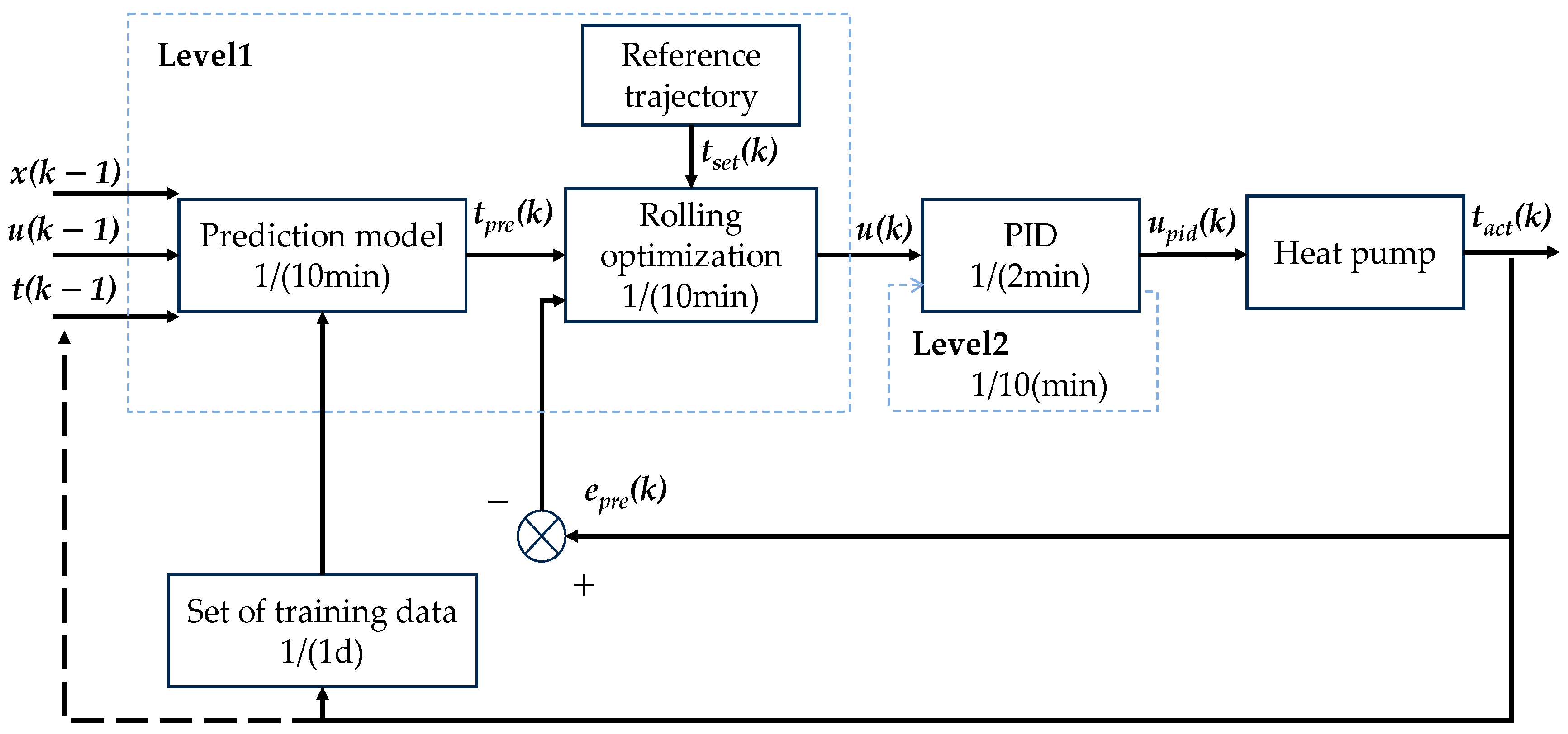
Therefore, to provide minutes-ahead frequency regulation services, we use the 2-level scheme shown in Figure 2. The scheme is an extension of Bünning et al. [35].
As shown in Figure 2, Level 1 is an MPC controller, which re-optimizes the base control quantity u ( k ) of the air-conditioning every ten minutes and reacts to unforeseen disturbances. t ( k 1 )   is the average indoor temperature during (k − 1) period, U k 1 is the duration of air conditioning control during (k − 1) period, x ( k 1 ) are other factors that affect indoor temperature during the (k − 1) period.
MPC utilizes a fixed time window dataset to predict the average indoor temperature for the next 10 min every 10 min and executes an optimization program to obtain the air conditioning control amount u ( k ) for the next period. u ( k ) is the total duration of control in the next 10 min.
Level 2 is a PID controller that regulates indoor temperature with a control cycle of 2 min. At the beginning of the first 2 min, determine whether the indoor temperature is within the set range. If it exceeds the upper limit, the system calculates the opening time U p i d _ 2 m i n through the PID and starts cooling. In other cases, no action is taken. Perform the same operation for the second 2 min until the end of 10 min. Total operation duration of the PID U p i d _ 10 m i n u ( k ) . When all execution is completed within 10 min of this period, feedback correction is performed using the measured values instead of the temperature values from the previous period to achieve closed-loop control.
The dataset of the prediction model consists of a training set, a validation set, and a testing set arranged in series. Three datasets are divided in an 8:1:1 ratio. Due to the fact that the actual production cycle of seafood mushrooms in the factory is 23 days, and the mushrooms are used for disinfection after being stored for 3 days without the need for air conditioning adjustment, the fixed total dataset length is 3312 pieces per 23 days and will be dynamically updated in the days thereafter. After generating 144 new data pieces per day, place them at the end of the test dataset and shift the remaining data upwards until all dataset updates are completed.

3.5. Data-Driven MPC

MPC is a model-based rolling horizon optimization control method consisting of three parts: a predictive model, an objective function, and an optimization algorithm [23]. Facing different practical problems, the prediction model and objective function are not the same.

3.5.1. Prediction Model

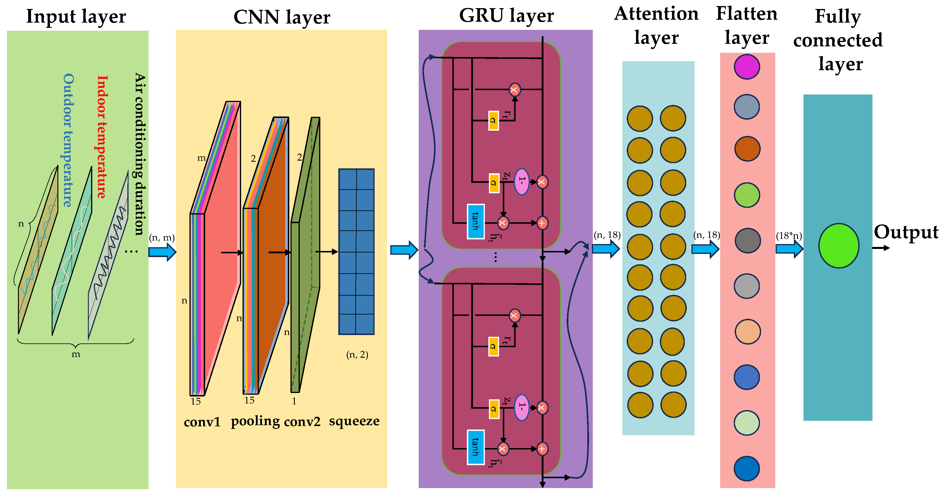
This article selects CNN-GRU-Attention as the prediction model for MPC. The model structure is mainly composed of an input layer, CNN layer, GRU layer, attention layer, and output layer. The detailed structure is shown in Figure 3.
  • Input layer: Preprocessing indoor and outdoor temperatures, air conditioning on time, etc., and then representing them as a two-dimensional matrix of time steps and eigenvectors, with a data dimension of [n,m] where n is the time step in the prediction model, and m is the number of input feature categories. Input 2D data into the prediction model.
  • CNN layer: After the input data is processed by the first convolutional layer and the spatiotemporal dimension features in the data are captured, the data dimension becomes [n,m,15]. After pooling, the data dimension becomes [n,2,15] and is sent to the second convolutional layer for processing. The data dimension becomes [n,2,1], and then a squeeze layer is added to compress the output dimension to [n,2] and output to the GRU layer. Both CNN layers use ReLU as the activation function.
  • GRU layer: Use L2 normal form regularization to prevent model overfitting. After processing, the data dimension becomes [n,18].
  • Attention layer: The attention layer enhances attention to important information through weighting.
  • Output layer: The flatten layer converts the output of the attention layer into global features, changes the data dimension to [18 × n], and then connects one fully connected layer to output the prediction results.
After determining the structure of the prediction model, the NSGA-II is used to optimize hyperparameters such as neuron count and learning rate. The detailed parameters of the neural network are shown in Table 1.

3.5.2. Objective Function and Control Optimization

Establish an objective function with the goal of achieving the lowest air conditioning energy consumption within the set temperature range. As shown in Formulas (6) and (7).
o b j 1 ( k ) = m i n i = 1 N [ t p r e ( k + i ) t s e t ( k + i ) ] 2
o b j 2 ( k ) = m i n i = 0 N 1 [ u ( k + i ) ] 2
where, t s e t ( k ) is the set temperature for the k period, u ( k ) is the total duration of air conditioning during the k period, o b j 1 ( k ) is the indicator of the control accuracy term for the k period, o b j 2 ( k ) is the indicator of energy consumption during the k-period.
This is a typical multi-objective solving problem. This article uses NSGA-II to solve the Pareto solution set of o b j 1 ( k ) and o b j 2 ( k ) . Then, use the entropy weight method to select a set of solutions from the Pareto solution set.
The parameter settings of the NSGA-II are shown in Table 2. Set the random number generated during the training process of the fixed model with random seeds to ensure the reproducibility of the model operation results.

3.5.3. Error Correction

Due to prediction errors and external interference factors, the accuracy of the prediction model will gradually deteriorate, and feedback compensation based on the prediction error is required.
After obtaining the actual temperature t a c t ( k ) and predicted temperature t p r e k during the k period, adjust the next prediction using the error between them. The prediction error is as follows (8):
t p r e k t a c t k = e p r e k
where, e p r e ( k ) is the error between the predicted temperature and actual temperature during period k.
Use this error to correct the predicted temperature in the next prediction, as shown in Formula (9):
t p r e k + 1 = t p r e k + 1 + e p r e k  
where, t p r e ( k + 1 ) is predicted temperature after (k + 1) period correction.

4. Results and Discussion

4.1. Analysis of Prediction Model Accuracy

4.1.1. Feature Selection

The original data includes nine input characteristics: indoor and outdoor temperature and humidity, solar radiation, wall heat flux, CO2 concentration, fresh air volume, and air conditioning duration.
A data-driven prediction model can accurately predict temperature, but redundant features require higher computational costs. To select the dataset most relevant to the predicted temperature, the Pearson correlation coefficient method and the Boruta method were used to screen the original dataset, where the Pearson correlation coefficient method was selected based on a correlation coefficient greater than 0.2. The Pearson correlation coefficient method excluded indoor and outdoor humidity, solar radiation, indoor CO2 concentration, and fresh air, while the Boruta method preserved indoor CO2 concentration.
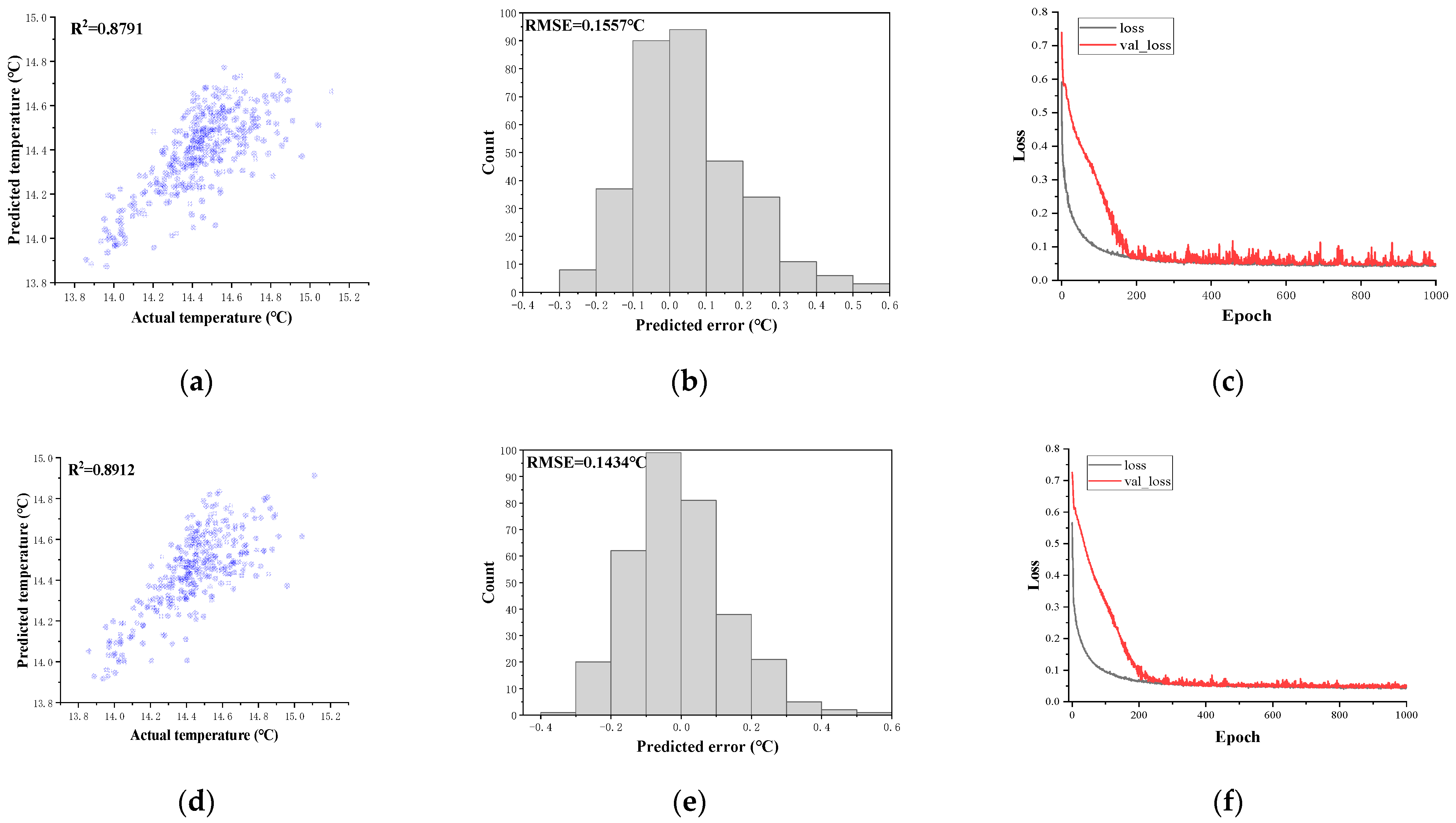
To evaluate the performance of two feature selection methods, the selected features are input into the prediction model for prediction. Assuming that the time step of the prediction model is determined to be 3, that is, using the average temperature data from historical periods of 0–10 min, 10–20 min, and 20–30 min to predict the temperature within the next 0–10 min. The constructed prediction models were evaluated using an evaluation dataset, which was 10% of the entire training dataset and not involved in the training process. The correlation analysis between the target and predicted data, error histograms, and changes in the loss values of the prediction model are shown in Figure 4.
The R2 value of the Pearson correlation coefficient method was 0.8791. The R2 value of the Boruta method was 0.8912. The RMSE value of the Pearson correlation coefficient method was 0.1557 °C for the predicted temperature and actual temperature. There was higher prediction accuracy for the Boruta method with results of 0.1434 °C. Compared with the Pearson correlation coefficient method, the Boruta method filtered dataset is applied to the prediction model, resulting in a smoother change in the loss value of the model.
Both methods reject indoor humidity and solar radiation. Due to the requirements of mushroom cultivation technology, the humidity inside the mushroom room has been maintained above 90% so that the indoor humidity will have little impact on the indoor temperature in the future. The solar radiation data is distorted due to the obstruction of surrounding trees. The heat flux of the enclosure structure can better reflect the impact of outdoor heat sources, such as temperature and solar radiation, on the temperature inside the mushroom room.
The Pearson correlation coefficient method excluded the CO2 concentration, indicating a weak linear relationship between the indoor temperature and CO2 concentration in the future. However, changes in the CO2 concentration during non-ventilation periods reflect the heat production of the edible fungi. As mentioned earlier, when the CO2 concentration in the internal air rises to 3500 ppm, exhaust air will also affect the indoor temperature.
Therefore, the Boruta method selects the optimal input feature set, reduces computational complexity, and improves the prediction accuracy of the prediction model.

4.1.2. Varying Time Step

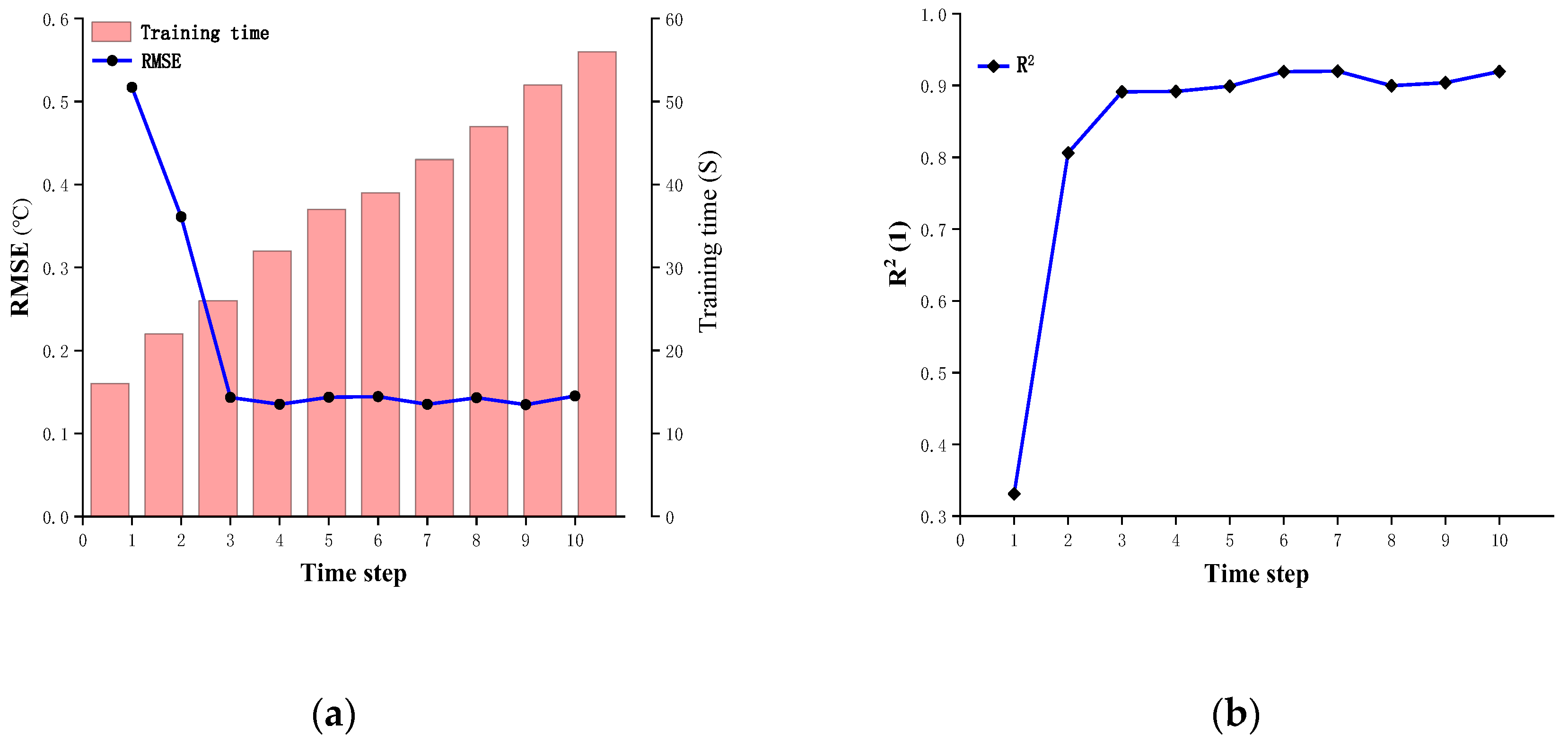
The time step size in the prediction model affects the prediction accuracy and training time of the model. This study was tested in time steps of 1–10. The results are shown in Figure 5.
When the time step is 1, the average temperature data from the historical 0–10 min period is used to predict the future 0–10 min temperature, with a prediction error of 0.517 °C and R2 of 0.331. The poor prediction effect is due to the large variation in temperature difference between indoors and outdoors during the summer in Beijing, with a delay time of more than 12 min for outdoor heat to enter the room through doors and ventilation windows. Using only the data from the above 10 min period as the input dataset for the prediction model cannot fully reflect the trend of indoor temperature changes in the future period. When the time step is 2, the prediction error is 0.361 °C, and R2 is 0.8061. The prediction error has significantly decreased, while R2 has significantly increased, indicating that the delay time is mostly concentrated within the range of 12–20 min. When the time step n ≥ 3, as n continues to grow, the prediction accuracy and determination coefficient tend to stabilize.
The training time of the prediction model is directly proportional to the time step n. When updating the dataset every day, the prediction model needs to be retrained once. After careful consideration, a time step of 3 is the best choice. It should be pointed out that the time reserved for decision-making in the proposed control method is 2 min, mainly composed of model prediction time and optimization time. The model prediction time is not the model training time, usually completed within 1 s, while the optimization time is generally relatively long. Detailed calculations will be introduced in Section 4.2.

4.2. Effect of the Prediction Horizon

Unlike the time step size in the prediction model, the prediction horizon reflects the MPC’s prediction of all information in the future period in the designed control model, which may include several prediction behaviors. When the prediction time domain is 1, use a once prediction model to predict the average temperature in the next 0–10 min. When the prediction time domain is 2, two consecutive prediction models are used to predict the average temperature in the next 0–10 min and 10–20 min, respectively, when the prediction time domain is 3, and so on. In this paper, the values in the control time domain and prediction time domain are the same. Control is the role of decision-making to constrain the total duration of the PID control within a 10 min period.
The selection of predictive and control time domain values has a significant impact on the performance of model predictive control.
To determine the appropriate control time domain, a control time range of 0–10 min, 0–20 min, 0–30 min, 0–40 min, 0–50 min was selected. Taking August 18th as an example, the average power consumption of air conditioning for one day was calculated, and the results are shown in Table 3.
When the control horizon is 0–10 min, the opening time of the air conditioning is 717.4 min. As the control horizon gradually increases, the energy consumption of air conditioning also gradually decreases and tends to stabilize.
Meanwhile, the computational complexity of model optimization increases with the increase in prediction range. When the computer performance is constant, the increase in computational load will further exacerbate the shortage of computing resources. The running time of the optimization algorithm is related to computer performance. In this study, the minimum control time period is 2 min, and the decision must be completed within the first 2 min. After careful consideration, 30 min is chosen as the control horizon.

4.3. Performance Verification

To verify the control effectiveness of the constructed control method, we compared it with the on/off thermostat and PID controller.
The control cycle of PID is 2 min, and the parameter K P is 0.02, K I is −0.9, K D is 0.02. The target temperature for all three methods is 14.5 °C. Taking July 16th as an example, the results are shown in Figure 6.
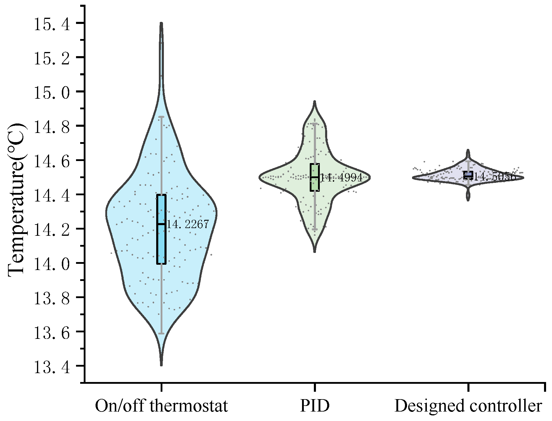
Figure 6 shows the range of indoor temperature fluctuations controlled using the on/off thermostat, PID controller, and designed controller in mushroom houses. The on/off thermostat controls the indoor temperature between 15.2831 and 13.5876 °C, with 25–75% data between 13.9948 and 14.3969 °C, with a median of 14.2267 °C. The PID controller controls the indoor temperature between 14.8376 and 14.1614 °C, with 25–75% data between 14.4203 and 14.5772 °C, with a median of 14.4994 °C. The designed controller controls the indoor temperature between 14.6403 and 14.3823 °C, with 25~75% data between 14.4558 and 14.5924 °C, with a median of 14.5056 °C. Compared with the switch method and PID method, the designed controller reduces the RMSE of controlling the temperature of the mushroom room by more than 90%.
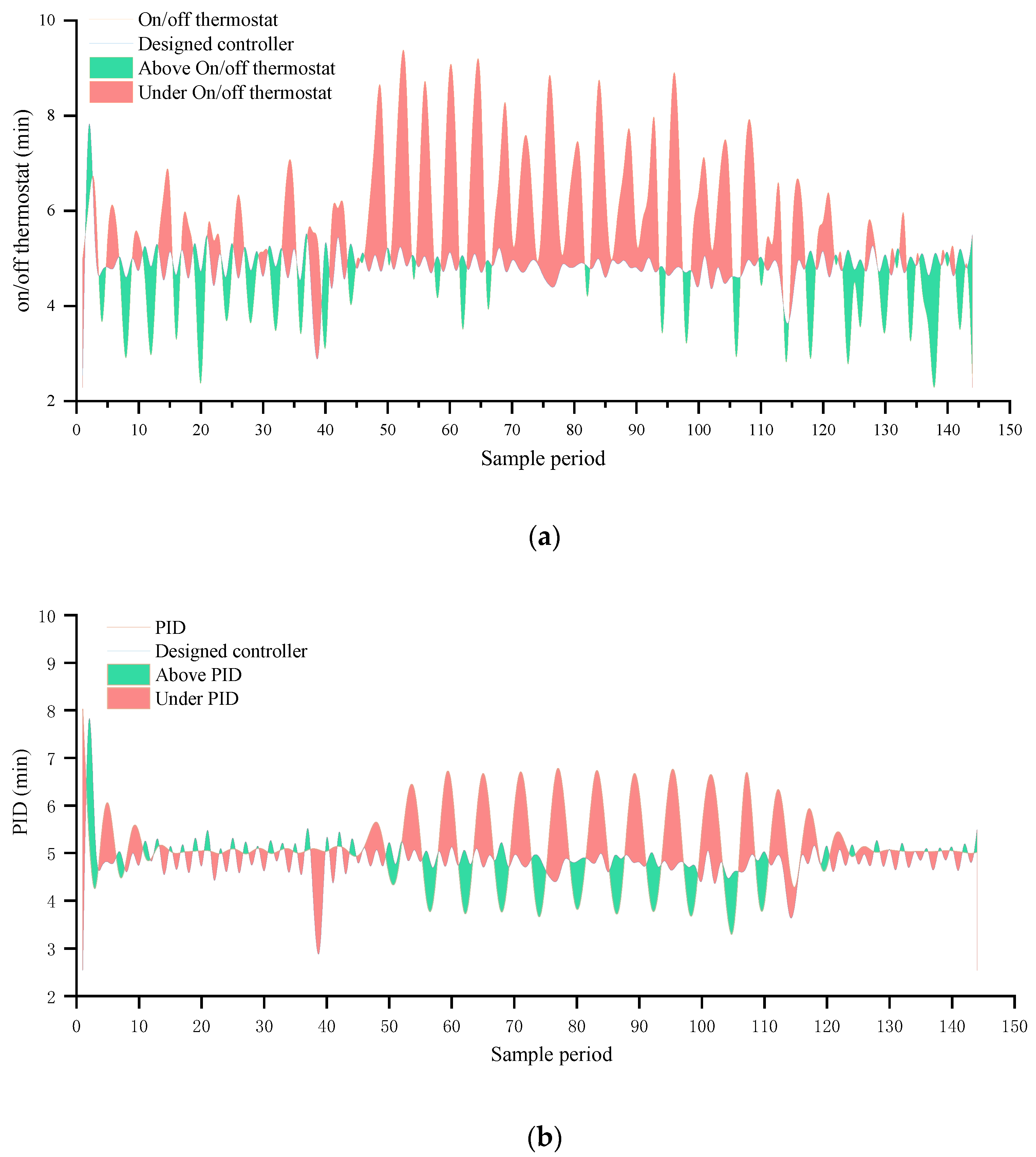
Figure 7 shows the cumulative opening time of the three controllers in one day. The opening time of the air conditioner under the statistical PID controller is 741 min, and the on/off thermostat is 797 min. The opening time of the designed controller is 701 min.
Compared with the on/off thermostat and PID controller, the designed controller reduces power consumption by 12% and 5%, respectively. The designed controller can track the set temperature without temperature overshoot and has better energy-saving effects than the other two methods.

5. Conclusions

This article designs a data-driven mushroom room air conditioning model predictive control method based on predictive models, rolling optimization, and feedback correction. This method combines the advantages of the PID and MPC, determines the optimal energy-saving decision quantity in the future period through MPC, and further uses the PID to control the start and stop of the air conditioning.
This article fully utilizes the accuracy advantages of a combination of neural networks and attention mechanisms in prediction, proposes the CNN-GRU-Attention as the prediction model in the controller, uses the Boruta algorithm to screen the input features of the model, and clarifies that the prediction model for indoor temperature in mushroom factories has the best effect in predicting the future 10 min of indoor temperature using historical 30 min data. It also utilizes prediction error compensation and dynamic updates of the prediction model dataset, Ensuring good prediction accuracy. The experiment shows that the predicted RMSE is 0.1434 °C and R2 is 0.8912.
According to the characteristics of the region, season, and thermal parameters of mushroom houses, the suitable control time domain for MPC has been determined.
Compared with the on/off thermostat and PID controller commonly used in edible mushroom factories, the controller method constructed in this study shows better control accuracy and energy-saving effects.
The prediction accuracy directly affects the energy-saving effect. Therefore, the future work plan includes fully exploring data features using feature decomposition methods such as empirical wavelet transform (EWT) before prediction and then using different prediction methods for different modal components to improve prediction accuracy. In addition, consideration will be given to incorporating the heat balance equation into the loss function of the prediction model to improve the robustness of the prediction data.

Author Contributions

Conceptualization, M.W. and W.Z.; methodology, M.W.; software, M.W.; validation, X.Z., Y.C. and C.C.; formal analysis, M.W.; resources, W.Z.; data curation, Y.C.; writing—original draft preparation, M.W.; writing—review and editing, M.W.; visualization, M.W.; supervision, C.Z. All authors have read and agreed to the published version of the manuscript.

Funding

The APC was funded by the Beijing Academy of Agricultural and Forestry Sciences Science and Technology Innovation Capacity Construction Project (KJCX20230410), the earmarked fund for CARS-20, Beijing Innovation Consortium of Agriculture Research System (BAIC03).

Data Availability Statement

Data are contained within the article.

Acknowledgments

The author would like to thank the anonymous reviewers for their constructive comments, which helped improve the quality of this paper.

Conflicts of Interest

The authors declare no conflict of interest.

References

  1. Guan, D.P.; Hu, Q.G. Energy saving analysis of industrial production of edible mushrooms. Edible Fungi 2010, 32, 1–3. [Google Scholar]
  2. Esmaeilzadeh, A.; Deal, B.; Yousefi-Koma, A.; Zakerzadeh, M.R. How Multi-Criterion Optimized Control Methods Improve Effectiveness of Multi-Zone Building Heating System Upgrading. Energies 2022, 15, 8675. [Google Scholar] [CrossRef]
  3. Jeon, B.K.; Kim, E.J. LSTM-Based Model Predictive Control for Optimal Temperature Set-Point Planning. Sustainability 2021, 13, 894. [Google Scholar] [CrossRef]
  4. Kim, D.; Lee, J.; Do, S.; Mago, P.J.; Lee, K.H.; Cho, H. Energy Modeling and Model Predictive Control for HVAC in Buildings: A Review of Current Research Trends. Energies 2022, 15, 7231. [Google Scholar] [CrossRef]
  5. Wang, D.; Chen, Y.Z.; Wang, W.G. Field test of Model Predictive Control in residential buildings for utility cost savings. Energy Build. 2023, 288. [Google Scholar] [CrossRef]
  6. Drgoňa, J.; Arroyo, J.; Cupeiro Figueroa, I.; Blum, D.; Arendt, K.; Kim, D.; Ollé, E.P.; Oravec, J.; Wetter, M.; Vrabie, D.L.; et al. All you need to know about model predictive control for buildings. Annu. Rev. Control 2020, 50, 190–232. [Google Scholar] [CrossRef]
  7. Yao, Y.; Shekhar, D.K. State of the art review on model predictive control (MPC) in heating ventilation and air-conditioning (HVAC) field. Build Env. 2021, 200, 107952. [Google Scholar] [CrossRef]
  8. Henze, G.P. Model predictive control for buildings: A quantum leap? J. Build. Perform. Simul. 2013, 6, 157–158. [Google Scholar] [CrossRef]
  9. Sangi, R.; Müller, D. A novel hybrid agent-based model predictive control for advanced building energy systems. Energy Convers. Manag. 2018, 178, 415–427. [Google Scholar] [CrossRef]
  10. Lee, H.; Heo, Y. Simplified data-driven models for model predictive control of residential buildings. Energy Build. 2022, 265, 1122067. [Google Scholar] [CrossRef]
  11. Killian, M.; Kozek, M. Ten Questions Concerning Model Predictive Control for Energy Efficient Buildings. Build. Environ. 2016, 105, 403–412. [Google Scholar] [CrossRef]
  12. Aruta, G.; Ascione, F.; Bianco, N.; Mauro, G.M.; Vanoli, G.P. Optimizing heating operation via GA-and ANN-based model predictive control: Concept for a real nearly-zero energy building. Energy Build. 2023, 292, 113139. [Google Scholar] [CrossRef]
  13. Kathirgamanathan, A.; De Rosa, M.; Mangina, E.; Finn, D.P. Data-driven predictive control for unlocking building energy flexibility: A review Renew. Sustain. Energy Rev. 2021, 135, 110120. [Google Scholar] [CrossRef]
  14. Afram, A.; Janabi-Sharifi, F.; Fung, S.A.; Raahemifar, K. Artificial neural network (ANN) based model predictive control (MPC) and optimization of HVAC systems: A state of the art review and case study of a residential HVAC system. Energy Build. 2017, 141, 96–113. [Google Scholar] [CrossRef]
  15. Serale, G.; Fiorentini, M.; Capozzoli, A.; Bernardini, D.; Bemporad, A. Model predictive control (MPC) for enhancing building and HVAC system energy efficiency: Problem formulation, applications and opportunities. Energies 2018, 11, 631. [Google Scholar] [CrossRef]
  16. Kumar, P.; Rawlings, J.B.; Wenzel, M.J.; Risbeck, M.J. Grey-box model and neural network disturbance predictor identification for economic MPC in building energy systems. Energy Build. 2023, 286, 112936. [Google Scholar] [CrossRef]
  17. Afram, A.; Janabi-Sharifi, F. Review of modeling methods for HVAC systems Appl. Therm. Eng. 2014, 2, 507–519. [Google Scholar] [CrossRef]
  18. Afram, A.; Janabi-Sharifi, F. Black-box modeling of residential HVAC system and comparison of grey-box and black-box modeling methods. Energy Build. 2015, 94, 121–149. [Google Scholar] [CrossRef]
  19. Stoffel, P.; Maier, L.; Kümpel, A.; Schreiber, T.; Müller, D. Evaluation of advanced control strategies for building energy systems. Energy Build. 2023, 280, 112709. [Google Scholar] [CrossRef]
  20. Qiang, G.; Zhe, T.; Yan, D.; Neng, Z. An improved office building cooling load prediction model based on multivariable linear regression. Energy Build. 2015, 107, 445–455. [Google Scholar] [CrossRef]
  21. Yun, K.; Luck, R.; Mago, J.P.; Cho, H. Building hourly thermal load prediction using an indexed ARX model. Energy Build. 2012, 54, 225–233. [Google Scholar] [CrossRef]
  22. Chen, Y.; Gao, J.; Yang, J.; Berardi, U.; Cui, G. An hour-ahead predictive control strategy for maximizing natural ventilation in passive buildings based on weather forecasting. Appl. Energy 2023, 333, 120613. [Google Scholar] [CrossRef]
  23. Lee, D.; Ooka, R.; Ikeda, S.; Choi, W.; Kwak, Y. Model predictive control of building energy systems with thermal energy storage in response to occupancy variations and time-variant electricity prices. Energy Build. 2020, 225, 110291. [Google Scholar] [CrossRef]
  24. Cox, S.J.; Kim, D.; Cho, H.; Mago, P. Real time optimal control of district cooling system with thermal energy storage using neural networks. Appl. Energy 2019, 238, 466–480. [Google Scholar] [CrossRef]
  25. Kato, K.; Sakawa, M.; Ishimaru, K.; Ushiro, S.; Shibano, T. Heat load prediction through recurrent neural network in district heating and cooling systems. In Proceedings of the 2008 IEEE International Conference on Systems, Man and Cybernetics, Singapore, 12–15 October 2008. [Google Scholar]
  26. Suryanarayana, G.; Lago, J.; Geysen, D.; Aleksiejuk, P.; Johansson, C. Thermal load forecasting in district heating networks using deep learning and advanced feature selection methods. Energy 2018, 157, 141–149. [Google Scholar] [CrossRef]
  27. Wang, D.; Han, C.; Wang, L.; Li, X.; Cai, E.; Zhang, P. Surface roughness prediction of large shaft grinding via attentional CNN-LSTM fusing multiple process signals. Int. J. Adv. Manuf. Technol. 2023, 126, 4925–4936. [Google Scholar] [CrossRef]
  28. Jung, H.D.; Kim, J.H.; Kim, Y.J.; Lee, S.T.; Park, H.S. Time-serial analysis of deep neural network models for prediction of climatic conditions inside a greenhouse. Comput. Electron. Agric. 2020, 173, 105402. [Google Scholar] [CrossRef]
  29. Ding, Z.; Chen, W.; Hu, T.; Xu, X. Evolutionary double attention-based long short-term memory model for building energy prediction: Case study of a green building. Appl. Energy 2021, 288, 116660. [Google Scholar] [CrossRef]
  30. Picard, D.; Drgoňa, J.; Kvasnica, M.; Helsen, L. Impact of the controller model complexity on model predictive control performance for buildings. Energy Build. 2017, 152, 739–751. [Google Scholar] [CrossRef]
  31. Nelson, J.R.; Johnson, N.G. Model predictive control of microgrids for real-time ancillary service market participation. Appl. Energy 2020, 269, 114963. [Google Scholar] [CrossRef]
  32. Nguyen, T.A.; Reiter, S.; Rigo, P. A review on simulation-based optimization methods applied to building performance analysis Appl. Energy 2014, 113, 1043–1058. [Google Scholar] [CrossRef]
  33. Wang, L.; Han, J.; Ma, F.; Li, X.; Wang, D. Accuracy design optimization of a CNC grinding machine towards low-carbon manufacturing. J. Clean. Prod. 2023, 406, 137100. [Google Scholar] [CrossRef]
  34. Ascione, F.; Bianco, N.; De Stasio, C.; Mauro, G.M.; Vanoli, G.P. Multi-stage and multi-objective optimization for energy retrofitting a developed hospital reference building: A new approach to assess cost-optimality. Appl. Energy 2016, 174, 37–68. [Google Scholar] [CrossRef]
  35. Bünning, F.; Warrington, J.; Heer, P.; Smith, R.S.; Lygeros, J. Robust MPC with data-driven demand forecasting for frequency regulation with heat pumps. Control Eng. Pract. 2022, 122, 105101. [Google Scholar] [CrossRef]
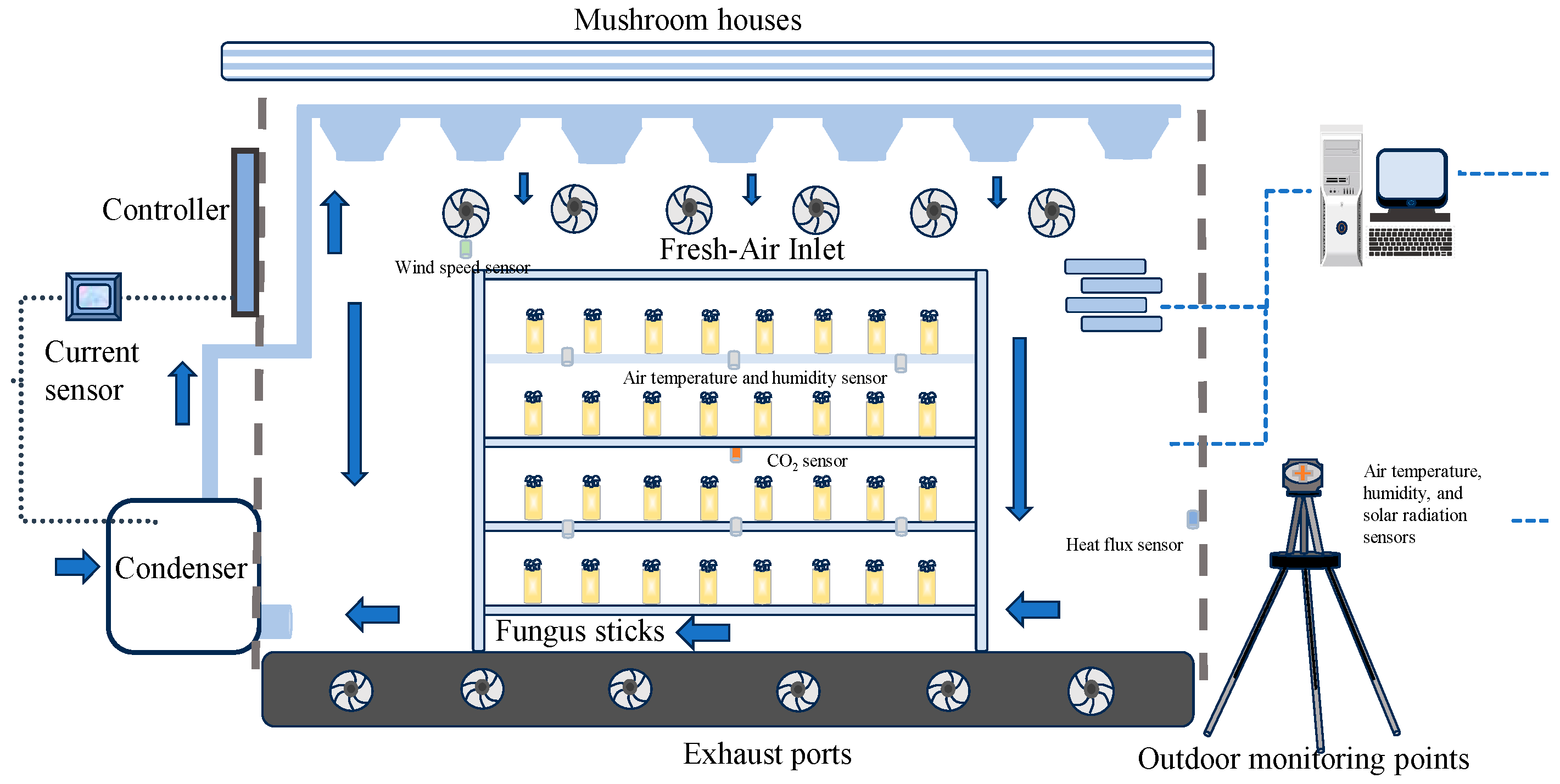
Figure 1. Schematic diagram of sensor installation in mushroom room.
Energies 16 07623 g001
Figure 2. Schematic diagram of the controller’s principle.
Energies 16 07623 g002
Figure 3. Structure diagram of the prediction model.
Energies 16 07623 g003
Figure 4. Performance evaluation of the prediction models under different feature sets. (a) The correlation analysis between the predicted target and the predicted data in the dataset selected using the Pearson correlation coefficient method. (b) The error histogram between the predicted target and the predicted data in the dataset selected using the Pearson correlation coefficient method. (c) The changes in model loss value in the training and validation sets selected using the Pearson correlation coefficient method. (d) The correlation analysis between the predicted target and the predicted data in the dataset selected using the Boruta method. (e) The error histogram between the predicted target and the predicted data in the dataset selected using the Boruta method. (f) The changes in model loss value in the training and validation sets selected using the Boruta method.
Energies 16 07623 g004
Figure 5. R2, RMSE, and training time of model at different time steps. (a) The RMSE and training time of the model at different time steps. (b) The R2 at different time steps.
Energies 16 07623 g005
Figure 6. Comparison diagram of the on/off thermostat, PID, and designed controller control temperature.
Energies 16 07623 g006
Figure 7. Comparison diagram of the air conditioning time controlled using the on/off thermostat, PID, and designed controllers. (a) Comparison of the on/off thermostat and designed controller; (b) comparison of the PID and designed controller.
Energies 16 07623 g007
Table 1. Neural network hyperparameter.
HyperparameterValue
Number of convolutional kernels in layer 115
Convolutional kernel size of layer 13 × 3
Pooled core size1 × 2
Number of convolutional kernels in layer 21
Convolutional kernel size of layer 23 × 3
Number of neurons in the GRU layer18
Learning rate0.001
Epoch1000
Batch size500
Table 2. Parameters of NSGA-II algorithm.
ParameterValue
Parent populations70
Offspring populations60
Crossover probability0.6
Mutation probability0.1
Iterations40
Table 3. The comparison of MPC different control horizons.
Control Horizon
(min)
Duration of Air Conditioning (min)Optimization Duration
(s)
0–1071743
0–2069660
0–3068685
0–40681131
0–50683156
Disclaimer/Publisher’s Note: The statements, opinions and data contained in all publications are solely those of the individual author(s) and contributor(s) and not of MDPI and/or the editor(s). MDPI and/or the editor(s) disclaim responsibility for any injury to people or property resulting from any ideas, methods, instructions or products referred to in the content.