Article

Decentralized Smart Grid Stability Modeling with Machine Learning

1
HEP Group, Distribution System Operator Ltd., Viktora Cara Emina 2, 51000 Rijeka, Croatia
2
Department of Automation and Electronics, Faculty of Engineering, University of Rijeka, Vukovarska 58, 51000 Rijeka, Croatia
*
Author to whom correspondence should be addressed.
Energies 2023, 16(22), 7562; https://doi.org/10.3390/en16227562
Submission received: 4 October 2023 / Revised: 10 November 2023 / Accepted: 12 November 2023 / Published: 14 November 2023
(This article belongs to the Special Issue Sustainable/Renewable Energy Systems Analysis and Optimization)

Abstract

:
Predicting the stability of a Decentralized Smart Grid is key to the control of such systems. One of the key aspects that is necessary when observing the control of DSG systems is the need for rapid control. Due to this, the application of AI-based machine learning (ML) algorithms may be key to achieving a quick and precise stability prediction. In this paper, the authors utilize four algorithms—a multilayer perceptron (MLP), extreme gradient boosting (XGB), support vector machines (SVMs), and genetic programming (GP). A public dataset containing 30,000 points was used, with inputs consisting of τ —the time needed for a grid participant to adjust consumption/generation, p—generated power, and γ —the price elasticity coefficient for four grid elements; and outputs consisting of s t a b —the eigenvalue of stability and s t a b f , the categorical stability of the system. The system was modeled using the aforementioned methods as a regression model (targeting s t a b ) and a classification model (targeting s t a b f ). Modeling was performed with and without the τ values due to their low correlation. The best results were achieved with the XGB algorithm for classification, with and without the τ values as inputs—indicating them as being unnecessary.

1. Introduction

The power system is a vertical structure that is divided into three parts: generation, transmission, and distribution. The power system operates on the principle that electricity is generated in distant power plants and then transmitted to consumers through power lines. A power system is expected to have high reliability, low cost, and satisfactory quality (constant frequency, voltage within certain limits, and a sinusoidal waveform) [1]. A wide range of methods and devices are used to meet these conditions and to achieve a high degree of efficiency and stability. Power flows in one direction from a few central generating units to a large number of consumers. However, the system shows signs of obsolescence when confronted with new challenges, such as rapid technological progress, the different profiles of market participants, and above all, a significant increase in generation from renewable energy sources (RESs) [2].
Improvements in RESs and various packages of measures proposed by the European Union (EU) in response to global climate change, such as the goal of achieving carbon neutrality by 2050 [3], have led to a sharp increase in the total power produced from those sources [4]. Key measures include the introduction of the Emissions Trading Scheme, the first major carbon market for trading emission rights requiring all large facilities in the energy, industrial, and aviation sectors to purchase emission permits to offset their carbon footprint [5]. Furthermore, the initial investment in RESs is partly financed by the EU, and RESs are given priority dispatch rights [6]. The aforementioned policies have led to an increased use of RESs, which has resulted in the decentralization of the power grid, problems of the controllability of power production [7], and an unintentional two-way flow of energy. These new conditions represented a threat to the integrity and stability of the power grid, and to rectify the mentioned shortcomings, the Smart Grid was introduced. Unlike the traditional power grid, the smart grid uses communication infrastructure and metering devices to achieve a two-way flow of energy and information. As a result, the price of electrical energy can be set by the power provider throughout the day based on information about the production and consumption of the participants connected to the grid [8]. However, such a centralized approach of information collection about the generation and consumption at each raises the question of data storage [9], cybersecurity [10], and communication standards [11], to name a few.
To be stable, electrical grids require the balance between production and consumption to be maintained. Traditionally, balance was maintained with demand-driven electricity production, but with the introduction of the Smart Grid, the demand response (DR) was established. The DR is based on flexible prices and assumes a change in energy consumption in relation to the price, i.e., low prices stimulate consumers to increase their consumption. The conventional approach in the form of electricity auctions is based on a centralized collection of information about production and consumption to negotiate the price of electrical energy every fifteen minutes. An alternative approach in the form of Decentralized Smart Grid Control (DSGC), a new type of smart grid has been proposed and tested by Schäfer et al. in 2015 [12] and 2016 [13], respectively, and later expanded upon by Arzamasov et al. (2018) [14]. In contrast, DSGC aims to achieve DR by using grid frequency to determine the price of electrical energy. This approach introduces a real-time price (as opposed to a fifteen-minute delay) and eliminates the need for communication equipment between participants connected to the grid, as the frequency can be measured easily. In power engineering, frequency is used as a benchmark to determine the balance between electrical energy production and consumption. When the production of electrical energy is higher than the consumption, the frequency increases and vice versa [15]. Depending on the deviation from the reference value, the price changes to stimulate producers and consumers to adjust their consumption or generation. When the frequency falls to below the reference value, the price increases to stimulate consumers to reduce their consumption, and during periods when the frequency is above the reference value, the price decreases to stimulate an increase in consumption.
This proposal, where the price is determined solely through the measurement of the local frequency, without central agency, has several mentioned benefits. However, the question of stability, in a system without central control, where grid participants themselves are responsible for maintaining grid stability with their energy consumption behaviors, can be raised. Considering that the stability of the DSGC system depends on the interdependency between the technical and economic subsystems, determining stability can become a complex task. For example, according to [12], a system without delay in adaption to demand τ = 0 is shown to be stable. However, in a more realistic scenario with delayed adaption, τ > 0 resonance can happen, driving the system to become unstable. However, it is shown that resonance can be prevented by introducing the averaging time T, during which the price is fixed. Furthermore, in [13], a DSGC system was expanded to include line capacity K and the price elasticity of consumers γ , i.e., the willingness of the customers to change consumption in response to a price change. The system stability was tested on various grid topologies with central and decentralized power production. In research, it was shown that decentralized production, a higher averaging time T, and a higher line capacity K have an important impact on stability; however, it was also shown that grid topology has an important impact on stability. For certain values of τ and T, the lattice-like grid will be stable, but the cycle-like grid will be unstable. However, the methodology used in [12,13] has two drawbacks. Firstly, during the simulation, only a value of τ varied, meaning that an interaction between other input values ( γ and T) was not considered. Secondly, the assumption that grid participants have the same input values is not realistic, as private households vary in energy consumption and cannot be regulated externally. To solve these shortcomings, Arzamasov et al. (2018) [14] have proposed using data-mining methods to obtain a diverse set of inputs to model grid participants with greater accuracy.
Artificial intelligence (AI) has been applied to solve several problems occurring in the power grid, such as load forecasting [16], voltage [17], transient stability [18], load shedding [19], etc. For example, Solyali et al. (2020) [16] have applied several machine learning (ML) algorithms to estimate electricity demand over the short term and long term. Data were collected every 15 minutes, with a long-term dataset consisting of 34,944 data points for the entire 2016 and 2017 periods, while the short-term dataset consisted of 673 data points for one week in January of 2016 and 2017. The input parameters for the ML algorithm were temperature, humidity, solar irradiation, population, gross national income (GNI), and the price of electrical energy. The best results were achieved with a support vector machine (SVM) with a Root Mean Square Error (RMSE) of 25.935 MW (4.49%) for the long term and with an artificial neural network (ANN) with a prediction error of 11.29 MW (1.67%) for the short term. Xi et al. (2021) [20] have proposed a deep reinforcement learning based three-network double-delay actor-critic (TDAC) based on the double deep Q network, a reinforcement learning (RL) algorithm. This approach comes as an alternative to proportional integral control, which is not suited to dealing with big fluctuations in energy production caused by RESs. For a real-time simulation with disturbance in the form of the step wave, square wave, and stochastic wave, TDAC has demonstrated a higher learning efficiency, stronger convergence characteristics, and better adaptability in the random environment.
Liu et al. (2021) [17] used iterated random forest to predict a static voltage stability margin. The suggested model contains offline training, feature preprocessing and selection, partial mutual information, and online prediction; and it managed to achieve an R 2 score of 0.9742 on IEEE’s 30-bus system and 0.9684 on a practical 1648-bus system. Moreover, Shi et al. (2020) [18] used a convolutional neural network (CNN) to predict transient stability. Similar papers have predicted stability in a binary fashion i.e., stable or unstable; however, this paper can not only assess if the system will be stable or unstable, but it can also distinguish types of instabilities such as aperiodic or oscillatory instability. This was also accomplished as an online assessment, meaning that grid operators are given enough time to react and to possibly prevent the instability of the system from happening. This was achieved by converting time series to grid-like data, which were then processed by CNN with 97.7% accuracy. Meng et al. (2020) [21] proposed using a decision tree (DT) based on the C4.5 algorithm for an online voltage stability assessment. Firstly, a power-voltage (P-V) curve analysis was is performed for various grid topologies and conditions to generate samples. To facilitate the stability assessment, only samples that are near the stability boundary are considered. Next, the relief algorithm is used to determine and reduce the number of features used for DT. Finally, the C4.5 algorithm is used to construct the DT on a dataset containing 628 samples, with several attributes varying from 34 to 164. The best result was achieved on 75 attributes, with a classification accuracy of 92.04%. In addition, according to Wang et al. (2019) [19], AI can be applied to assess frequency stability. This paper proposes the serial integration of model-driven and data-driven models, which are then combined with an integrated method consisting of system frequency response (SFR) and extreme learning machine (ELM) into a procedure for predicting frequency dynamics and load shedding. The SFR model was applied in the preservation of frequency response characteristics, while ELM was used to predict a load-shedding amount. A New England 39-bus system integrated method using both SFR and ELM resulted in an MAE of 0.033 Hz for maximum frequency deviation and an MAE of 0.009 Hz for steady-state frequency. Furthermore, Amroune et al. (2020) [22] used dragonfly optimization (DFO) in tandem with support vector regression (SVR). The voltage values on the buses were used as an input value, while the voltage stability index was used as the output value for SVR. The DFO algorithm was used for finding optimal SVR parameters, as their selection is crucial for achieving good performance. The hybrid model was tested on IEEE 30-bus and Algerian 59-bus systems with an RMSE value of 0.0273 and 0.0565, respectively. Another example of the system stability estimation is given by An and Yang (2018) [23], in which the authors introduce a switching function matrix into the observer design. In a case where a possible destabilization is detected, the observer shuts off the inputs which may be causing the issues, with the authors providing examples of cyber-attacks on sensor networks.
Reports have been made on the prediction of voltage [17,21,22], frequency [19], and transient stability [18]; however, due to the unique approach of the DSGC to DR, it is difficult to make a comparison to results regarding the stability of traditional power grid. The stability of the DSGC system is a question of predicting whether grid participants with their energy consumption behavior cause resonance by increasing and decreasing power consumption, a question that was answered in traditional power grids with a centralized oversight of power providers. Even though several scientific papers have been published on the topic of DSGC thus far, an extensive analysis of AI in the stability prediction of DSGC was not a focus of any recently published research.
Therefore, the following research questions are raised:
  • Is it possible to estimate the stability of the DSGC system with high performance using AI-based models?
  • What are the hyperparameters of the AI algorithms used that provide satisfactory results or otherwise the best-achieved results within the scope of this research?
  • Is it possible to use a stacking ensemble made up of previously used algorithms to achieve a higher performance in obtaining regression and classification models for addressing the problem of stability prediction?
The main motivation of this paper is to present not only the model for the prediction of the stability of a DSGC system, but to determine the manner in which the highest-performing model can be developed. This refers to the method used in the model generation and between the four evaluated models, as well as determining whether a higher level of performance can be achieved when the models are developed for the regression or the classification tasks. The importance of this lies in the development of models on more advanced datasets—whether they are simulated datasets that are based on a more realistic schemes of users (namely, a significantly larger amount of participants in the network than the four used in this research) or on real, collected, datasets from actual DSG networks.
This paper is split into four sections. Section 2 will describe the process by which the dataset was generated, as well as its analysis, along with the description of the utilized modeling methodology. In Section 3, the results of the two approaches—the single algorithm approach for four different algorithms and the stacking ensemble approach are presented and discussed. Finally, the answers to the posed research questions, along with research limitations and possible future directions, are presented in Section 4.

2. Materials and Methods

The materials and methods of this paper, namely the dataset used for the research, and the modeling and evaluation techniques, will be presented in this section.

2.1. Dataset Description

The dataset used in the research is presented, first by describing the model used for generation, and then followed by the description and statistical analysis of the dataset.

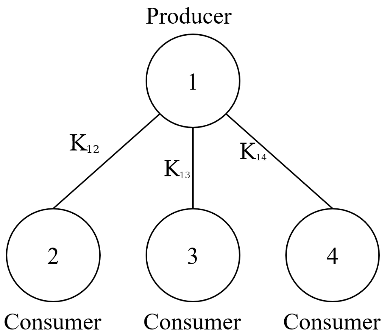
2.1.1. The Mathematical Model of the DSGC System

The DSGC system is modeled as an oscillator model by Schafer et al. [13], with the producers being represented by synchronous generators and the consumers as synchronous motors, similar to the Structure Preserving Model [24]. The model of the DSGC system is split into two parts: simulating the energy produced and consumed by participants connected to the grid and modeling the change in electrical energy price with respect to the grid frequency [12].
The energy dynamics of a synchronous machine can be described as [14]:
P S o u r c e = P A c c u m u l a t e d + P L o s s + P C o n s u m e d ,
where P S o u r c e refers to the power of the electrical energy source, consisting of accumulated power ( P A c c u m u l a t e d ), power lost during the transfer ( P L o s s ), and the power actually consumed by the client ( P C o n s u m e d ). It can be observed that the energy produced equals the sum of accumulated energy in rotating mass, energy losses, and energy consumed by the end users. The former equation can be expanded as [14]:
P j S o u r c e = 1 2 M j d d t ( δ j ) 2 + κ j ( δ j ) 2 k = 1 N P j k m a x s i n ( δ k δ j ) j { 1 , , N } ,
with M being a moment of inertia, κ being the coefficient of friction, P m a x being the capacity of the line, and δ being the rotor angle with j and k denoting the participants in the grid. Each synchronous machine can be described with rotor angle δ j ( t ) relative to the grid frequency and angular frequency deviation ω i = d θ i d t from a reference grid rotating at Ω = 2 π · 50 Hz [14]:
δ j ( t ) = ω t + θ j ( t ) ,
where ω is a grid frequency and θ j ( t ) is a relative rotor angle. When Equation (3) is substituted in Equation (2), and it is assumed that K j k = P j k m a x M j ω , α j = 2 κ j M j and P j = P j S o u r c e κ j ω 2 M j [14]:
d 2 θ j d t 2 = P j α j d θ j d t k = 1 N K j k s i n ( θ k θ j ) ,
with K j k being coupling strength of the maximal power that can be transmitted by the power lines, α j is the damping constant calculated as α j = 2 κ j M j , and P j is the mechanical power (with a negative value representing consumption and a positive value production). N represents the maximum number of participants k, within the grid.
The second part of modeling DSGC represents a change in the consumption of electrical energy in tandem with grid frequency (or price, which is proportional). Such a variable price of electrical energy can be described as a linear function of price and frequency P j [13]:
P j d θ j d t = p Ω c 1 d θ j d t .
The previous equation p Ω represents the price of electrical energy in steady state d θ j d t 0 , and c 1 ( c j ) represents the coefficient proportional to a price elasticity. Even though the reaction of participants connected to the grid is complex, it is assumed that there is a linear correlation between energy use and price P ^ j ( p j ) [13]:
P ^ j ( p j ) P j + c j ( p j p Ω ) ,
where p j is the price of electrical energy for user j, P ^ j is the quantity of energy produced or consumed, priced at p j . By substituting Equation (5) into Equation (6) and defining γ j = c 1 · c j as a factor that is proportional to the price elasticity of each node j, a change in mechanical power (as consumption or production) is bound to a change in frequency d θ j d t [13]:
P ^ j ( t ) = P j + γ j ( p j p Ω ) ( t ) , j { 1 , , N } .
with γ j being the measurement of participants’ willingness to adjust their consumption or production for node j [25,26]. Generally, an adjustment to a new price will not be instantaneous, but with a certain time delay τ , which is made up of the time needed to measure frequency, as well as the time needed for participants to act. Therefore, P ^ j ( t ) from Equation (7) is substituted with P ^ j ( t τ ) , inserted into Equation (4), and the equation with time delay τ is given as [13]:
d 2 δ j d t 2 = P j α j d θ j d t k = 1 N K j k s i n ( θ k θ j ) γ j d θ j d t ( t τ ) , j { 1 , , N } ,
However, a system with a large time delay poses a risk to the stability of the power grid. For instability to be avoided, Equation (8) is expanded with the averaging time T j , as seen in Equation (9), with the time interval T, during which the frequency (and with it, the price) are averaged over. Based on the average frequency, the system stability is periodically determined, no matter the specific time delay of each producer or consumer [13]:
d 2 δ j d t 2 = P j α j d θ j d t k = 1 N K j k s i n ( θ k θ j ) γ j T j ( θ j ( t τ j ) θ j ( t τ j T j ) ) , j { 1 , , N } .
The DSGC is defined by the six input values. Three of these are the control parameters set by the system designer when the system is being initialized and include: coupling strength K j k , damping factor α j , and averaging time T j . To simplify the calculation, it is assumed that the coupling strength between the nodes is identical and that all participants have equal moments of inertia. According to equation α j = 2 κ j M j , this also means that the damping factor α j will be identical for all nodes. The second category is environmental parameters whose values differ from case to case, such as the generated/consumed power P j and the time delay τ j . The third input parameter γ j is composed of two values, c 1 , and c j . The value c 1 is a control value linking the price of electric energy and the grid frequency, while c j is variable and indicates the extent to which each grid participant j is willing to adjust its consumption or generation.
The values chosen for the control parameters are the averaging time T = 2 s, the coupling strength K j k = 8 s 2 , and the damping factor α j = 0.1 s 1 . The variable parameters values are defined with limits, the power consumed by the consumer P j = [−0.5, −2] s 2 , the price elasticity γ j = [0.05, 1] s 1 , and the grid participant reaction time τ = [0.5, 10] s 1 , as shown in Table 1. In order to simulate the diverse set of inputs, the values of parameters which can be varied were selected randomly using Latin Hypercube Sampling [14,27].
After defining the input values, the method of determining system stability must be chosen. Stability analysis can be performed with several methods, such as stability against single perturbations, basin stability, and linear stability. For determining system stability, linear stability analysis was chosen since it does not add additional variables to an already complex system [14]. Linear stability analysis of the dynamic system is used to determine stability near the steady-state operation of the system determined by the eigenvalues of Equation (9). This equation has infinitely many solutions, but only a finite number of solutions have a real positive part that determines the instability of the system [13]. If the maximum value of the eigenvalue has a negative value, the system is considered stable for that particular case and vice versa.

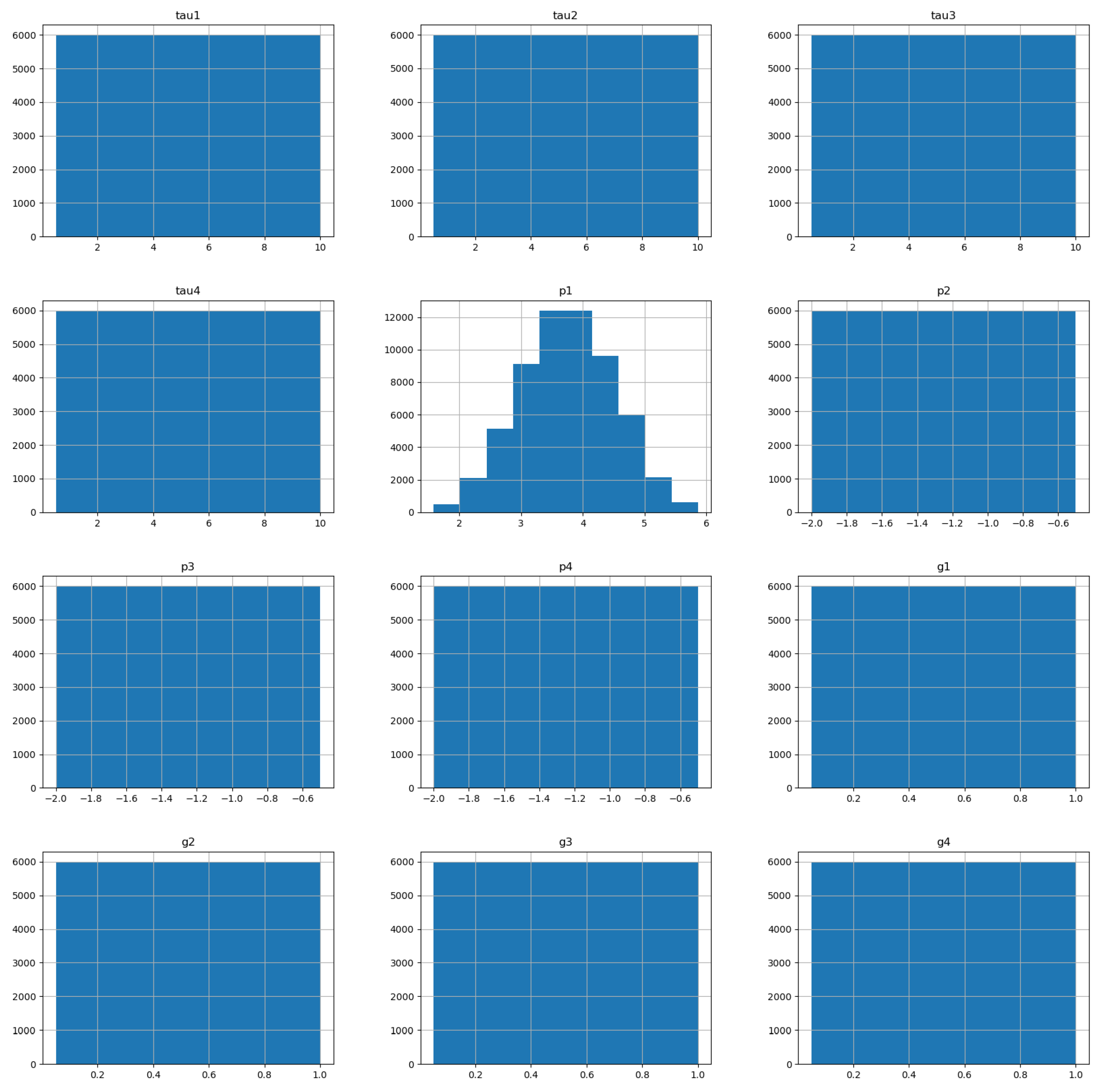
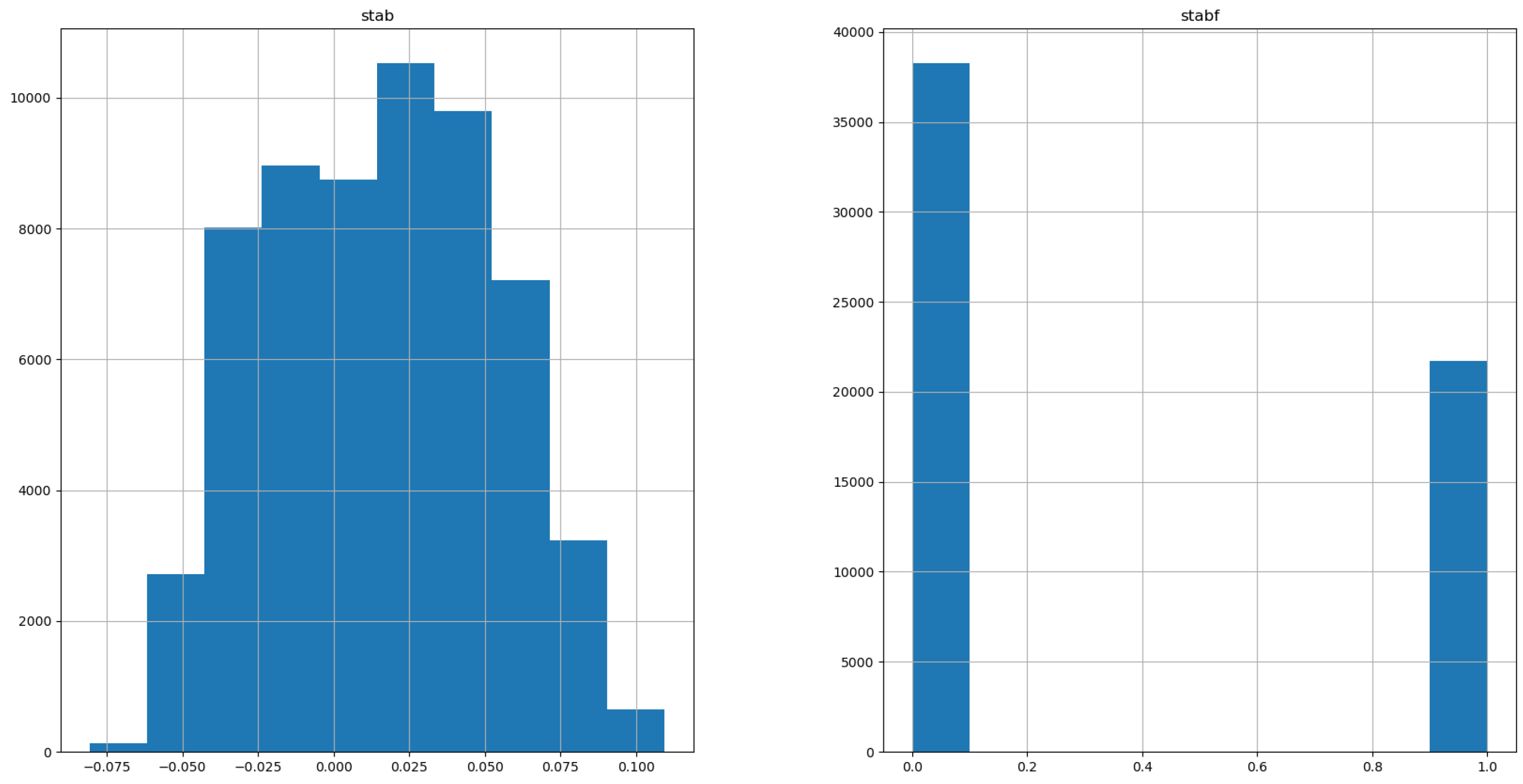
2.1.2. Description and Analysis of the Dataset Used 

In this paper, the dataset used for model development is publicly available and created by Breviglieri [28] as an augmented version of Arzamasov’s dataset [29], expanded from 10 thousand to 60 thousand data points. Arzamasov et al. (2018) [14] simulated the DSGC system 10,000 times using the input values specified in Table 1. The simulation was based on one producer node and three consumer nodes connected in a star topology, as seen in Figure 1. The data points were obtained via the described methodology of simulation given in the previous subsection. The individual data points were created through the random selection of values for the input variables given further in the dataset description and the calculation of the system stability based on the simulations.
The dataset consists of twelve input values that correspond to the values given in the mathematical description of the model above:
  • τ i , i [ 1 , 2 , 3 , 4 ] —the time needed for a grid participant to adjust consumption or generation (8),
  • p i , i [ 1 , 2 , 3 , 4 ] —the power generated (positive value) or consumed (negative value) (2),
  • γ i , i [ 1 , 2 , 3 , 4 ] —the price elasticity coefficient (7).
The inputs [1, 2, 3, 4] represent possible grid participants, with 1 denoting the producer node and the others denoting consumer nodes. The dataset also consists of two output values,
  • s t a b —the stability of the systems, represented as an eigenvalue of the Equation (9) for that set of input values, as a numerical value,
  • s t a b f —the stability of the system as a categorical value divided between two states, ‘stable’ and ‘unstable’.
It is worth noting that s t a b represents the maximum eigenvalue of Equation (9), meaning that the system will have a categorical value of ‘unstable’ for every data point with a positive eigenvalue, and a value of ‘stable’ for the negative eigenvalue.
A basic statistical analysis was performed on the target dataset and can be seen in Table 2. The difference between the minimum and maximum values of the dataset is small, and considering that a high degree of accuracy was achieved, different methods of normalization and scaling were not applied.
To visually represent the values in the dataset used, histograms of values have been plotted. In Figure 2, we can see that most variables are distributed uniformly across their entire range. The only exception to this is p 1 which has a regular triangular distribution.
The histograms of the two versions of the output variable are given in Figure 3. ‘stabf’ shows that there are more ‘unstable’ than ‘stable’ data points in the dataset, but the difference is not significant to the point where it could cause issues. Observing the distribution of ‘stab’, we can see that the distribution of the system is roughly normal, although it is not completely regular. This is especially interesting as most of the inputs are regularly distributed, indicating that the connection between inputs and outputs is complex.
Additionally, correlation analysis of the dataset was performed by using Spearman’s rank correlations. Spearman’s correlation is used to assess the monotonic relationships between two variables, and it ranges between −1.0 and 1.0. A correlation value of 1.0 between two variables means that if the value of the one variable increases, so will the value of the second one, with the opposite being true.
In Figure 4, a heatmap of correlation values can be seen. A negligible correlation between the input values can be observed, except for moderate correlation between p 1 , p 2 , p 3 , and p 4 , which is to be expected, considering that the equation p 1 = p 2 + p 3 + p 4 was conditioned from the start of the simulation. Furthermore, there is a negligible correlation between the input and output values, with a correlation of 0.28 between s t a b and t a u , and 0.29 between s t a b and g. Moreover, an even lower correlation can be observed between p and s t a b , with the average correlation being 0.006. This coincides with Arzamasov’s [14] findings, who concluded that power has small or no impact at all on system stability. Therefore, a question is raised: is it possible to achieve a higher performance on a dataset without that variable than it is on a full dataset?
The p-value of the Spearman rank correlation denotes the chance that the observed relationship is a result of coincidence. Determined from the correlation value and the sample size, the p-values range from 0 to 1.0 with low p values, meaning that there is a low chance of the correlation being a coincidence and vice versa [30]. As can be seen from Figure 5, the p-values between t a u i , s t a b , g i , and s t a b are zero, meaning that there is little to no chance of the correlation being falsely positive.

2.2. Methods

The main goal of this paper is to determine the ability of AI algorithms to develop models for stability prediction with DSGC. For this purpose, various types of AI algorithms were used, such as multilayer perceptron, support vector machine, gradient boosting machine, and genetic programming, in both regression and classification as a single algorithm and an ensemble approach.
To obtain a result with a high degree of accuracy, a randomized hyperparameter search with cross-validation was used. In the first step, the values of the hyperparameters are chosen at random, and the model is validated using five-fold cross-validation. In the process of cross-validation, the dataset is split into a k-number of subsets (in the case of five-fold cross-validation, k = 5). Then, each subset is used as a testing set, while the remaining subsets are used as a training dataset [31]. In the end, a set of hyperparameters that achieved the highest average score for a certain model is then repeated in the same manner in order to determine the metrics that are later described in this paper. To more easily understand this process, it has been illustrated in Figure 6.

2.2.1. Multilayer Perceptron

Multilayer perceptron (MLP) is a type of feedforward artificial neural network with supervised learning, used to perform a non-linear approximation for both the regression and classification tasks. The MLP consists of neurons arranged into three types of layers—input, output, and hidden. The first layer is the input layer made of the same number of neurons as input variables, or in the case of this research, twelve neurons. Layers between the input and output layers are called hidden layers, consisting of weighted neurons followed by an activation function. Lastly, the output layer transforms values from the last hidden player to output values. Considering the fact the MLP can estimate a single value, the output layer consists of a single neuron [31].
MLP uses weight factors of hidden layers to estimate the output value. In the beginning, the values of the weight factors are chosen randomly. However, during the training, based on the error of a forward propagated result, the weights are corrected proportionally to the error in the process of backpropagation [32]. The MLP used in this paper was ‘MLPRegressor’ for regression and ‘MLPClassifier’ for classification problems. The hyperparameters taken into consideration and their ranges are showcased in Table 3.
The hyperparameter ‘hidden_layer_sizes’ represents how many hidden layers there are and how many neurons the hidden layer contains, while the hyperparameter ‘activation’ denotes the activation function used at the end of the hidden layer. The hyperparameter ‘solver’ is used to choose a solver for weight optimization, and the hyperparameter ‘alpha’ is a strength of the L2 regularization term. The hyperparameters ‘beta_1’ and ‘beta_2’ denote the exponential decay rate for estimates of the first and second vector for solver Adam. The hyperparameter ‘learning_rate_init’ controls the step size in updating the weights, and ‘epsilon’ is the value of numerical stability for solver ‘adam’.

2.2.2. Support Vector Machine

The support vector machine (SVM) is a supervised learning algorithm that can be used in classification, regression, and outliers detection. The SVM is based on the method in which input vectors are set in a high-dimensional feature space Z. The decision surface is then calculated to ensure a highly efficient grouping of input vectors. The optimal hyperplane, defined as a decision function that separates vectors into two or more groups with maximum margin, is then calculated. To calculate the optimal hyperplane, only a small fraction of training data determining the margins of the hyperplane are taken into consideration; these are called support vectors. The SVM used for classification uses only a small part of the training data because the modeling process ignores the training points beyond the margin. Similar to this, support vector regression uses a subset of data because the model ignores training points that are close to their targets [33]. The SVM-based methods used include “SVR” for regression and ‘SVC’ for classification problems. The hyperparameters taken into consideration and their ranges are showcased in Table 4.
The hyperparameter ‘kernel’ is used to pick the kernel function used to determine the optimal hyperplane; for example, if ‘linear’ is chosen as a kernel function, the hyperplane will be estimated using the linear function. The hyperparameter ‘degree’ is used to determine the degree of the polynomial function and it is used in conjunction with ‘poly’ kernel, and ‘gamma’ determines the influence of a single training example, with a higher value of ‘gamma’, meaning that points need to be very close to each other to be grouped together. The hyperparameter ‘coef0’ denotes an independent term in kernel function and it is used only in the ‘poly’ and ‘sigmoid’ kernels, and the hyperparameter ‘epsilon’ defines epsilon-tube, a distance within which no penalty is given to the training loss function if the predicted value is located within that distance from the actual value. The hyperparameter ‘C’ parameter is used as a trade-off between the misclassification of training examples and the simplicity of the decision surface [22].

2.2.3. Gradient Boosting Machine

Gradient boosting machine (GBM) is an AI method used to solve regression and classification problems. GBM combines several decision trees to create the final model. These trees are built in series, meaning that each tree rectifies the error present in the prediction values of the previous tree. This means that the GBM is based on a combination of several simple models, also known as weak learners. After the new decision tree is constructed, the model’s build residual is calculated per:
y i f ( x i ) y i ^ ,
where y i is the target value, f ( x i ) is the predicted value, and y i ^ is the residual. By calculating residuals, feedback is given to model how close the predicted value is to the target value. The expression defining the new tree is given as:
f = f 0 + α f 1 ,
with α being the learning rate hyperparameter. The residual is then recalculated based on the new decision tree f 2 , which attempts to correct the error made by tree f 1 :
f = f 0 + α f 1 + α f 2 ,
This process repeats until the defined maximum number of trees is reached. Trees can also be built below each other, determined by the depth of the tree’s hyperparameter. Increasing the depth results in longer training and prediction times, but it makes the model more accurate [34]. The GBM used in the scope of this paper is ‘XGBRegressor’ for regression and ‘XGBClassifier’ for classification problems. Hyperparameters taken into consideration and their ranges are showcased in Table 5.
The hyperparameter ‘eta’ determines the step size shrinkage after each boosting step. ‘eta’ shrinks the feature weights to make the boosting process more conservative, preventing overfitting, while the hyperparameter ‘max_depth’ denotes the maximum depth of a tree created by the model. Additionally, the hyperparameter ‘min_child_weight’ determines the weight needed to continue partitioning the tree with the leaf nodes; hyperparameter ‘lambda’ is an L2 and ‘alpha’ is an L1 regularization term on weights. Increasing the values of both hyperparameters results in the model being more conservative. The hyperparameters ‘colsample_bytree’, ‘colsample_bylevel’, and ‘colsample_bynode’ determine how many columns of the dataset will be subsampled for each tree, depth level, and node (split), and the hyperparameter ‘num_parallel_tree’ indicates several parallel trees being constructed during each iteration [35].

2.2.4. Genetic Programming

Genetic programming (GP) is a method combining evolutionary computation and machine learning used to solve regression and classification problems. GP is based on the concept of evolving the population of a mathematical formula that uses input values and mathematical operations to predict the output value. Computer programs are represented by syntax trees, made up of internal nodes and leaves. The leaves of a tree are constants and variables called terminals. The internal nodes are represented by arithmetic and trigonometric functions (e.g., addition, subtraction, and sine function), and they are called functions. In more complex cases, the GP model can be made up of several trees connected to a special root node. Those (sub)trees are called branches and together with other features, they create the architecture of the GP model [36].
At the start of GP, an initial population is created randomly. Using such a randomly created population results in low accuracy. To increase the model performance, an evolution process is performed on the population. To determine accuracy, a fitness function is used. The fitness function is the primary mechanism for determining the accuracy of every unit for each generation. There are multiple methods of determining which of the units will be evolved, but the most common one is the so-called tournament selection [36]. In the tournament selection, units are chosen at random to compete in the tournament. Units compete in pairs, with units that have higher fitness having a better chance of winning the tournament. As a result, units that have higher fitness values have more children on average. Since units participating in the tournament are chosen at random, diversity is maintained, otherwise only a couple of the best units would be constantly selected for evolution, leading to sub-optimal results. The unit that is selected after the tournament selection process evolves using evolutionary computing (EC) operators. The EC operators used in this research are crossover and mutation. The crossover operator creates a child program by taking a random subtree from the winner and replacing it with a randomly created subtree. The mutation operator evolves the single-parent program by changing randomly selected nodes, subtrees, or a leaf. In GP, genetic operators are mutually exclusive, meaning that a single genetic operator is used on the selected units in one iteration [36]. The GP used in the scope of this paper is a “Symbolic Regressor” for regression and a “Symbolic Classifier” for classification problems. The hyperparameters taken into consideration and their ranges are showcased in Table 6.
The hyperparameter “population_size” denotes the number of individual solutions (equations, models) and the hyperparameter “generations” is used to limit the number of generations during which programs evolve. The parameter “tournament_size” determines the number of programs that will compete in a tournament. The hyperparameter “Init_depth” describes the tree depth for the initial population, while the hyperparameter “init_method” determines the initialization method. In the initialization method, “grow” nodes are chosen at random from both functions and terminals; in the “full” method, functions are chosen until “init_size” is reached and then terminals are selected. Lastly, in the “half and half” method, trees are grown through a 50/50 mixture of ‘grow’ and ‘full’ methods. The hyperparameter “parsimony_coefficient” is a factor that penalizes large computer programs by reducing their fitness score. This allows for the “bloat” of the programs (an increase in program size) to be controlled [37].
All of the methods described in the previous paragraphs are are used to separately attempt and regress the dataset outputs, both as classifiers and regressors. The predicted output values will be compared for evaluation, with the goal of determining which is the best performing method for the dataset used in this research and similar datasets.

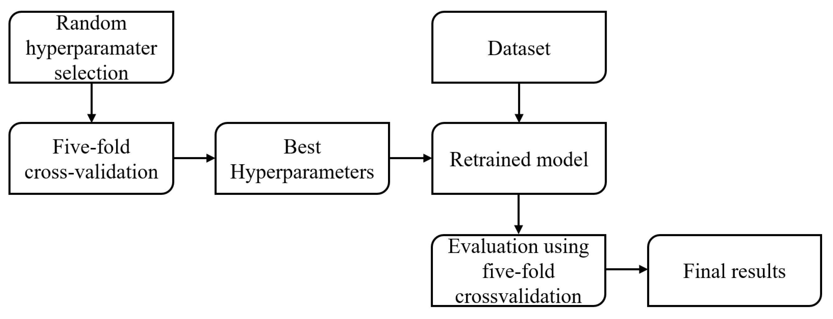
2.3. Model Evaluation

Evaluation metrics have a role in determining the performances of the AI models used. As different metrics can illustrate different types of errors, multiple metrics are used to obtain more information on the model’s performance. Due to the inherent difference between the regression and classification methods, separate methods are used for each.

2.3.1. Regression Evaluation Metrics

The regression results were evaluated with a coefficient of determination ( R 2 ). The R 2 score defines how well the variance, existing in the real data, is explained with the predicted data. The R 2 score ranges from 0 to 1, with a score of 1.0 meaning that all of the variances are explained in the predicted data [31].
R 2 = 1 i = 1 n ( X i Y i ) 2 i = 1 n ( X i Y i ¯ ) 2 .

2.3.2. Classification Evaluation Metrics

There are four different outcomes in the evaluation performance of the binary classification model: true positive ( T P ) when a positive result is predicted as positive, true negative ( T N ) when a negative result is predicted as negative, false positive ( F P ) when a negative result is predicted as positive, and false negative ( F N ) when a positive result is predicted as negative. Based on these four cases, two metrics can be calculated, precision and recall:
Precision = T P T P + F P ,
and recall, defined as:
Recall = T P T P + F N .
The values of both metrics range from 0 to 1.0, with 1.0 being the most desirable score. For a simpler representation, the precision and recall metrics can be combined into an F1 score and calculated as:
F 1 score = 2 × P r e c i s i o n × R e c a l l P r e c i s i o n + R e c a l l .

3. Results and Discussion

All of the simulations performed for obtaining models and the results were performed using the Python 3.11.4 programming language. The main implementation of the MLP and SVM algorithms used was from the Scikit-learn 1.3.2 library. Genetic programming implementation came from the Gplearn 0.4.2 library, and the gradient boosted trees implementation used the XGBoost 2.0.1 library. The described metrics and evaluation techniques (e.g., grid search and cross-validation) were also used as implemented in the aforementioned version of Scikit-learn. In Table 7, the results for both modeling tasks across all different algorithms used can be seen. Observing regression, the best results are achieved for the model developed with the XGB algorithm, with an R 2 score of 0.98 ± 0.0007. Comparably but with lower scores, results are achieved with the MLP algorithm, achieving an R 2 score of 0.97 ± 0.0024. SVM and GP achieve significantly lower scores. Observing the hyperparameters for the methods that achieved the results in question, both algorithms used relatively large models, with MLP using a five-layer-deep neural network with 200 neurons in each of the layers and XGB using the maximal tree depth of 9. This indicates that the modeling problem was complex. Comparing the classification results, it is obvious that similar trends follow—with XGB and MLP achieving the highest performing models— F 1 = 0.99 ± 0.02 when rounded to the second significant digit. The remaining two methods show a massive improvement, with SVM achieving an F 1 score of 0.96 and a GP of 0.84.
In Table 8, the results are shown for the experiment in which the models were trained, having removed the ‘ t a u 1’, ‘ t a u 2’, ‘ t a u 3’, and ‘ t a u 4’ inputs, due to their low correlation values. For the regression, the scores remained largely unchanged. While the performance did not improve, it must be noted that it also did not show a drop after four inputs were removed, confirming that they were largely unnecessary for achieving the models. As for the classification task, this remained true—no drop in values was present, and only a somewhat significant increase was seen in the case of the SVM classifier, which had a positive increase in F 1 score; Δ F 1 S V M = 0.0266 .

4. Conclusions

In this paper, the authors have attempted to create models for the prediction of DSGC system stability based on the set of inputs consisting of time for adjusting the consumption/generation cycle, power, and price elasticity coefficient. The dataset, consisting of 30,000 data points, was analyzed, and based on the correlation coefficients, two sets of inputs were used for modeling separately—with and without the time necessary for the adjustment of the consumption/generation cycle. Modeling was performed by targeting the value of the stability coefficient with regression, and through classification between the ‘stable’ and ‘unstable’ states. Modeling was performed with four different methods. The results demonstrate that classification achieves higher scores on average compared to the regression. The best score, F 1 = 0.9979 ± 0.0015, was achieved with the XGB algorithm for the classification without τ input values. For the regression, the best score was also achieved with an XGB of R 2 = 0.9820 ± 0.0007 . While this model did use τ as inputs, the comparative score without τ inputs ( R 2 = 0.9815 ± 0.0007) falls within the error range. Of the other methods, MLP has achieved satisfactory scores, SVM only achieved a satisfactory score for classification without τ , and GP did not achieve any satisfactory scores. Based on the achieved results, the following can be concluded. Stability prediction based on the aforementioned input values is possible, and it can achieve high-performance models using ML-based methods, namely XGB and MLP. The value of the τ inputs is not necessary for such modeling—removing it nets nearly equal or, in the case of SVM classification, improved results.

Author Contributions

Conceptualization, B.F. and N.A.; methodology, B.F.; software, S.B.Š.; validation, N.A., S.B.Š. and Z.C.; formal analysis, N.A.; investigation, B.F.; resources, S.B.Š.; data curation, N.A.; writing—original draft preparation, B.F. and N.A.; writing—review and editing, S.B.Š. and Z.C.; visualization, B.F.; supervision, N.A.; project administration, Z.C.; funding acquisition, Z.C. All authors have read and agreed to the published version of the manuscript.

Funding

This research has been (partly) supported by the CEEPUS network CIII-HR-0108, European Regional Development Fund under the grant KK.01.1.1.01.0009 (DATACROSS), project CEKOM under the grant KK.01.2.2.03.0004, the Erasmus+ project WICT under the grant 2021-1-HR01-KA220-HED-000031177, and the University of Rijeka scientific grant uniri-tehnic-18-275-1447 and uniri-mladi-technic-22-61.

Data Availability Statement

The data presented in this study are openly available in the Smart Grid Stability Kaggle repository, available at: https://www.kaggle.com/datasets/pcbreviglieri/smart-grid-stability (accessed on 1 October 2023).

Conflicts of Interest

Author Borna Franović was employed by the Distribution System Operator Ltd. The remaining authors declare that the research was conducted in the absence of any commercial or financial relationships that could be construed as a potential conflict of interest.

References

  1. Kundur, P.S.; Malik, O.P. Power System Stability and Control; McGraw-Hill Education: New York, NY, USA, 2022. [Google Scholar]
  2. Weedy, B.; Cory, B.; Jenkins, N.; Ekanayake, J.; Strbac, G. Electric Power Systems; Wiley: Hoboken, NJ, USA, 2012. [Google Scholar]
  3. Plötz, P.; Wachsmuth, J.; Gnann, T.; Neuner, F.; Speth, D.; Link, S. Net-Zero-Carbon Transport in Europe until 2050—Targets, Technologies and Policies for a Long-Term EU Strategy; Fraunhofer Institute for Systems and Innovation Research ISI: Karlsruhe, Germany, 2021; Available online: https://www.isi.fraunhofer.de/en.html (accessed on 25 July 2021).
  4. Golombek, R.; Lind, A.; Ringkjøb, H.K.; Seljom, P. The role of transmission and energy storage in European decarbonization towards 2050. Energy 2022, 239, 122159. [Google Scholar] [CrossRef]
  5. Verde, S.F. The impact of the EU emissions trading system on competitiveness and carbon leakage: The econometric evidence. J. Econ. Surv. 2020, 34, 320–343. [Google Scholar] [CrossRef]
  6. Sioshansi, F.P. Evolution of Global Electricity Markets: New Paradigms, New Challenges, New Approaches; Academic Press: Cambridge, MA, USA, 2013. [Google Scholar]
  7. Wang, J.; Zhong, H.; Wu, C.; Du, E.; Xia, Q.; Kang, C. Incentivizing distributed energy resource aggregation in energy and capacity markets: An energy sharing scheme and mechanism design. Appl. Energy 2019, 252, 113471. [Google Scholar] [CrossRef]
  8. Tuballa, M.L.; Abundo, M.L. A review of the development of Smart Grid technologies. Renew. Sustain. Energy Rev. 2016, 59, 710–725. [Google Scholar] [CrossRef]
  9. Tu, C.; He, X.; Shuai, Z.; Jiang, F. Big data issues in smart grid—A review. Renew. Sustain. Energy Rev. 2017, 79, 1099–1107. [Google Scholar] [CrossRef]
  10. El Mrabet, Z.; Kaabouch, N.; El Ghazi, H.; El Ghazi, H. Cyber-security in smart grid: Survey and challenges. Comput. Electr. Eng. 2018, 67, 469–482. [Google Scholar] [CrossRef]
  11. Colak, I.; Sagiroglu, S.; Fulli, G.; Yesilbudak, M.; Covrig, C.F. A survey on the critical issues in smart grid technologies. Renew. Sustain. Energy Rev. 2016, 54, 396–405. [Google Scholar] [CrossRef]
  12. Schäfer, B.; Matthiae, M.; Timme, M.; Witthaut, D. Decentral smart grid control. New J. Phys. 2015, 17, 015002. [Google Scholar] [CrossRef]
  13. Schäfer, B.; Grabow, C.; Auer, S.; Kurths, J.; Witthaut, D.; Timme, M. Taming instabilities in power grid networks by decentralized control. Eur. Phys. J. Spec. Top. 2016, 225, 569–582. [Google Scholar] [CrossRef]
  14. Arzamasov, V.; Böhm, K.; Jochem, P. Towards concise models of grid stability. In Proceedings of the 2018 IEEE International Conference on Communications, Control, and Computing Technologies for Smart Grids (SmartGridComm), Aalborg, Denmark, 29–31 October 2018; pp. 1–6. [Google Scholar]
  15. Kruse, J.; Schäfer, B.; Witthaut, D. Revealing drivers and risks for power grid frequency stability with explainable AI. Patterns 2021, 2, 100365. [Google Scholar] [CrossRef]
  16. Solyali, D. A comparative analysis of machine learning approaches for short-/long-term electricity load forecasting in Cyprus. Sustainability 2020, 12, 3612. [Google Scholar] [CrossRef]
  17. Liu, S.; Shi, R.; Huang, Y.; Li, X.; Li, Z.; Wang, L.; Mao, D.; Liu, L.; Liao, S.; Zhang, M.; et al. A data-driven and data-based framework for online voltage stability assessment using partial mutual information and iterated random forest. Energies 2021, 14, 715. [Google Scholar] [CrossRef]
  18. Shi, Z.; Yao, W.; Zeng, L.; Wen, J.; Fang, J.; Ai, X.; Wen, J. Convolutional neural network-based power system transient stability assessment and instability mode prediction. Appl. Energy 2020, 263, 114586. [Google Scholar] [CrossRef]
  19. Wang, Q.; Li, F.; Tang, Y.; Xu, Y. Integrating model-driven and data-driven methods for power system frequency stability assessment and control. IEEE Trans. Power Syst. 2019, 34, 4557–4568. [Google Scholar] [CrossRef]
  20. Xi, L.; Wu, J.; Xu, Y.; Sun, H. Automatic generation control based on multiple neural networks with actor-critic strategy. IEEE Trans. Neural Netw. Learn. Syst. 2020, 32, 2483–2493. [Google Scholar] [CrossRef]
  21. Meng, X.; Zhang, P.; Xu, Y.; Xie, H. Construction of decision tree based on C4.5 algorithm for online voltage stability assessment. Int. J. Electr. Power Energy Syst. 2020, 118, 105793. [Google Scholar] [CrossRef]
  22. Amroune, M.; Bouktir, T.; Musirin, I. Power system voltage stability assessment using a hybrid approach combining dragonfly optimization algorithm and support vector regression. Arab. J. Sci. Eng. 2018, 43, 3023–3036. [Google Scholar] [CrossRef]
  23. An, L.; Yang, G.H. Secure state estimation against sparse sensor attacks with adaptive switching mechanism. IEEE Trans. Autom. Control 2017, 63, 2596–2603. [Google Scholar] [CrossRef]
  24. Bergen, A.R.; Hill, D.J. A structure preserving model for power system stability analysis. IEEE Trans. Power Appar. Syst. 1981, PAS-100, 25–35. [Google Scholar] [CrossRef]
  25. Nimalsiri, N.I.; Mediwaththe, C.P.; Ratnam, E.L.; Shaw, M.; Smith, D.B.; Halgamuge, S.K. A survey of algorithms for distributed charging control of electric vehicles in smart grid. IEEE Trans. Intell. Transp. Syst. 2019, 21, 4497–4515. [Google Scholar] [CrossRef]
  26. Gangale, F.; Mengolini, A.; Onyeji, I. Consumer engagement: An insight from smart grid projects in Europe. Energy Policy 2013, 60, 621–628. [Google Scholar] [CrossRef]
  27. Stein, M. Large sample properties of simulations using Latin hypercube sampling. Technometrics 1987, 29, 143–151. [Google Scholar] [CrossRef]
  28. Breviglieri, P. Smart Grid Stability. 2020. Available online: https://www.kaggle.com/datasets/pcbreviglieri/smart-grid-stability (accessed on 25 January 2023).
  29. Arzamasov, V. Electrical Grid Stability Simulated Data Data Set. 2018. Available online: https://www.kaggle.com/datasets/ishadss/electrical-grid-stability-simulated-data-data-set (accessed on 11 November 2023).
  30. Akoglu, H. User’s guide to correlation coefficients. Turk. J. Emerg. Med. 2018, 18, 91–93. [Google Scholar] [CrossRef] [PubMed]
  31. Car, Z.; Baressi Šegota, S.; Anđelić, N.; Lorencin, I.; Mrzljak, V. Modeling the spread of COVID-19 infection using a multilayer perceptron. Comput. Math. Methods Med. 2020, 2020, 5714714. [Google Scholar] [CrossRef]
  32. Bishop, C.M. Pattern recognition and feed-forward networks. In The MIT Encyclopedia of the Cognitive Sciences; MIT Press: Cambridge, MA, USA, 1999; Volume 13. [Google Scholar]
  33. Suthaharan, S.; Suthaharan, S. Support vector machine. In Machine Learning Models and Algorithms for Big Data Classification: Thinking with Examples for Effective Learning; Springer: New York, NY, USA, 2016; pp. 207–235. [Google Scholar]
  34. Burkov, A. The Hundred-Page Machine Learning Book; Andriy Burkov: Quebec City, QC, Canada, 2019; Volume 1. [Google Scholar]
  35. Nguyen-Sy, T.; Wakim, J.; To, Q.D.; Vu, M.N.; Nguyen, T.D.; Nguyen, T.T. Predicting the compressive strength of concrete from its compositions and age using the extreme gradient boosting method. Constr. Build. Mater. 2020, 260, 119757. [Google Scholar] [CrossRef]
  36. Poli, R.; Langdon, W.B.; McPhee, N.F.; Koza, J.R. A Field Guide to Genetic Programming. With Contributions by JR Koza. 2008. Available online: https://www.zemris.fer.hr/~yeti/studenti/izvori/A_Field_Guide_to_Genetic_Programming.pdf (accessed on 4 October 2023).
  37. Anđelić, N.; Baressi Šegota, S.; Glučina, M.; Lorencin, I. Classification of Wall Following Robot Movements Using Genetic Programming Symbolic Classifier. Machines 2023, 11, 105. [Google Scholar] [CrossRef]
Figure 1. Nodal system of simulated Decentralized Smart Grid Control model.
Energies 16 07562 g001
Figure 2. Histograms of the input variables.
Energies 16 07562 g002
Figure 3. Histograms of the output variables.
Energies 16 07562 g003
Figure 4. Spearman’s rank correlation coefficient.
Energies 16 07562 g004
Figure 5. p Value of Spearman’s rank correlation coefficient.
Energies 16 07562 g005
Figure 6. Flowchart of the methodology used.
Energies 16 07562 g006
Table 1. Input values of the DSGC system and their values.
InputDescriptionTypeChosen Value
α j Damping constantControl input0.1 s 1
K j k Coupling strengthsControl input8 s 2
T j Averaging timeControl input2 s
γ j Price elasticityEnvironmental input[0.05, 1.00]
τ j Reaction timeEnvironmental input[0.5, 10]
P j Mechanical powerEnvironmental input[−0.5, −2]
Table 2. Table containing statistical description of the dataset used.
MeanStdMinMaxUnique Values
Input values t a u 15.252.740.5010.0010,000
t a u 25.252.740.5010.0030,000
t a u 35.252.740.5010.0030,000
t a u 45.252.740.5010.0030,000
p13.750.751.585.8610,000
p2−1.250.34−2.00−0.5030,000
p3−1.250.34−2.00−0.5030,000
p4−1.250.34−2.00−0.5030,000
g10.520.270.051.0010,000
g20.530.270.051.0030,000
g30.530.270.051.0030,000
g40.530.270.050.1130,000
Output values s t a b 0.020.04−0.080.1110,000
s t a b f stable 36%unstable 64%2
Table 3. Used hyperparameters for ‘MLPRegressor’ and ‘MLPClassifier’ models with their possible values expressed as a range or discreetly.
HyperparameterRange of Values
‘hidden_layer_sizes’(50,50,50,50,50,50,50,50,50,50),
(75,75,75,75,75,75,75,75,75),
(80,80,80,80,80,80,80,80),
(90,90,90,90,90,90,90),
(100,100,100,100,100,100),
(200,200,200,200,200)
‘activation’‘identity’, ‘logistic’, ‘tanh’, ‘relu’
‘solver’‘lbfgs’, ‘adam’
‘alpha’[0.0001–0.001]
‘beta_1’[0–0.9]
‘beta_2’[0.9–0.999]
‘learning_rate_init’[0.0001–0.001]
‘epsilon’ 1 × 10 9 1 × 10 7
Table 4. Used hyperparameters for ‘SVR’ and ‘SVC’ models, with their possible values expressed as a range or discreetly.
HyperparameterRange of Values
‘kernel’‘linear’, ‘poly’, ‘rbf’, ‘sigmond’
‘C’[0–100]
‘degree’[2, 3, 4, 5]
‘gamma’[0.001, 10]
‘coef0’[0, 1]
‘epsilon’[0.001–1]
Table 5. Used hyperparameters for ‘XGBRegressor’ and ‘XGBClassificator’ models, with their possible values expressed as a range or discreetly.
HyperparameterRange of Values
‘eta’[0–1]
‘max_depth’[4–10]
‘min_child_weight’[0–1]
‘max_delta_step’[1–10]
‘colsample_bytree’[0–1]
‘colsample_bylevel’[0–1]
‘colsample_bynode’[0–1]
‘num_parallel_tree’[1–5]
Table 6. Name of hyperparameters, range of values, and chosen values for ‘Symbolic Regressor’ and “Symbolic Classifier”.
HyperparameterRange of Values
population_size[1000–2000]
generations[200–1000]
tournament_size[50–500]
init_depth[2-3]–[5-7]
init_method‘grow’, ‘full’, ‘half and half’
parsimony_coefficient[0.001–0.01]
Table 7. Results of the random hyperparameter search for the regression problem.
Regression
AlgorithmAverage ScoreDeviationChosen Hyperparameters
MLP0.97720.0025learning_rate_init = 0.0001,
hidden_layer_sizes = (200, 200, 200, 200, 200),
epsilon = 1.8 × 10 8 , beta_2 = 0.936,
beta_1 = 0.3, alpha = 0.0001, activation = relu
SVM0.87090.0015kernel = poly, gamma = 0.219, epsilon = 0.042,
degree = 3, coef0 = 2.2, C = 46
XGB0.98200.0007subsample = 0.9, num_parallel_tree = 4,
min_child_weight = 0.5, max_depth = 9,
max_delta_step = 9, eta = 0.4,
colsample_bytree = 0.9, colsample_bynode = 0.7,
colsample_bylevel = 1.0
GP0.0620.0526tournament_size = 300, population_size = 1300,
parsimony_coefficient = 0.001, init_method = ‘full’,
init_depth = (2, 6), generations = 900
Classification
AI AlgorithmAverage ScoreStandard DeviationChosen Hyperparameters
MLP0.99300.0026solver = lbfgs, hidden_layer_sizes = (50,50,50,50,50),
activation = logistic
SVM0.95990.0007kernel = poly, gamma = 0.007, degree = 3, coef0 = 0, C = 28
XGB0.99340.0022subsample = 0.9, num_parralel_tree = 4,
min_child_weight = 0.9, max_depth = 10,
max_delta_step = 5, eta = 0.9, colsample_bytee = 0.2,
colsample_bylevel = 0.6, colsample_bynode = 0.9
GP0.84140.0208tournament_size = 50, population_size = 800,
parsimony_coefficient = 0.001, init_method = full,
init_depth = (3, 7), generation = 300
Table 8. Results of the random hyperparameter search for the classification problem.
Regression
AI AlgorithmAverage ScoreStandard DeviationChosen Hyperparameters
MLP0.97940.0008solver = adam, learning_rate_init = 0.0001,
hidden_layer_sizes = (200, 200, 200, 200, 200),
epsilon = 1.7 × 10 8 , beta_2 = 0.9,
beta_1 = 0.7, alpha = 0.00018, activation = relu
SVM0.85020.0080kernel = poly, gamma = 1.082, epsilon = 0.039,
degree = 4, coef0 = 7.0, C = 49
XGB0.98150.0007subsample = 0.6, num_parallel_tree = 4,
min_child_weight = 0.8, max_depth = 9,
max_delta_step = 8, eta = 0.4,
colsample_bytree = 0.8, colsample_bynode = 0.2,
colsample_bylevel = 1.0
GP0.0680.0565tournament_size = 300, population_size = 1300,
parsimony_coefficient = 0.001, init_method = ‘full’,
init_depth = (2, 6), generations = 900
Classification
AI AlgorithmAverage ScoreStandard DeviationChosen Hyperparameters
MLP0.99330.0006hidden_layer_sizes = (50, 50, 50, 50, 50, 50, 50, 50, 50, 50),
activation = identity, solver = lbfgs
SVM0.98650.0005kernel = rbf, gamma = 0.062, C = 100
XGB0.99700.0015subsample = 0.9, num_parralel_tree = 4,
min_child_weight = 0.0, max_depth = 10,
max_delta_step = 9, eta = 0.9, colsample_bytee = 0.3,
colsample_bylevel = 0.8, colsample_bynode = 0.5
GP0.84220.0198tournament_size = 50, population_size = 800,
parsimony_coefficient = 0.001, init_method = full,
init_depth = (3, 7), generation = 300
Disclaimer/Publisher’s Note: The statements, opinions and data contained in all publications are solely those of the individual author(s) and contributor(s) and not of MDPI and/or the editor(s). MDPI and/or the editor(s) disclaim responsibility for any injury to people or property resulting from any ideas, methods, instructions or products referred to in the content.

