Article

Wave Power Prediction Based on Seasonal and Trend Decomposition Using Locally Weighted Scatterplot Smoothing and Dual-Channel Seq2Seq Model

1
China Southern Power Grid Technology Co., Ltd., Guangzhou 510060, China
2
State Key Laboratory of Alternate Electrical Power System with Renewable Energy Sources, School of New Energy, North China Electric Power University, Beijing 102206, China
*
Author to whom correspondence should be addressed.
These authors contributed equally to this work.
Energies 2023, 16(22), 7515; https://doi.org/10.3390/en16227515
Submission received: 13 October 2023 / Revised: 7 November 2023 / Accepted: 8 November 2023 / Published: 9 November 2023
(This article belongs to the Section A3: Wind, Wave and Tidal Energy)

Abstract

:
Wave energy has emerged as a focal point in marine renewable energy research. Accurate prediction of wave power plays a pivotal role in enhancing power supply reliability. This paper introduces an innovative wave power prediction method that combines seasonal–trend decomposition using LOESS (STL) with a dual-channel Seq2Seq model. The decomposition model addresses the issue of component redundancy in current input decomposition methods, thereby uncovering key components. The prediction model improves upon the limitations of current prediction models that directly concatenate multiple features, allowing for a more detailed consideration of both trend and periodic features. The proposed approach begins by decomposing the power sequence based on tidal periods and optimal correlation criteria, effectively extracting both trend and periodic features. Subsequently, a dual-channel Seq2Seq model is constructed. The first channel employs temporal pattern attention to capture the trend and stochastic fluctuation information, while the second channel utilizes multi-head self-attention to further enhance the extraction of periodic components. Model validation is performed using data from two ocean buoys, each with a five-year dataset. The proposed model achieves an average 2.45% reduction in RMSE compared to the state-of-the-art method. Both the decomposition and prediction components of the model contribute to this increase in accuracy.

1. Introduction

Ocean energy holds vast prospects for development and is being closely scrutinized as a significant renewable energy source [1]. Wave energy shares similarities with wind and solar energy in terms of its renewable and environmentally friendly characteristics. The average wave energy density in most global marine areas exceeds 10 kW/m [2], indicating the substantial exploitable energy inherent in these fluctuations, thus endowing wave energy with significant energy storage potential. Considering that oceans cover 71% of the Earth’s surface, the widespread distribution of wave energy receives substantial attention on a global scale. Currently, wave energy converters (WECs) are experiencing rapid development, with many advanced WECs undergoing testing or deployment, such as the Wave Dragon WEC, Kaimei WEC, and TAPCHAN WEC [3,4].
The inherent variability, intermittency, and randomness of wave energy pose challenges to the stability of WECs’ power output. Grid dispatch requires reliable future power generation information to establish appropriate future power allocation. Wave energy generation is a viable option for powering islands and coastal cities [5], but the instability of its output presents a potential threat to the safe operation of small island grids. As WECs will be integrated into coastal city grids on a larger scale in the future, the issue of power output instability will become even more pronounced. Therefore, accurate prediction of wave energy generation is crucial for providing effective power output information to the grid, facilitating grid dispatch optimization, and enhancing the stability of the power system. Predictions are also essential for optimizing the operation of mechanical, electrical, and control systems in wave energy devices to enhance system efficiency.

1.1. Recent Investigations

Significant progress has been achieved in forecasting wind and solar power, with numerous forecasting systems deployed worldwide in wind farms and solar power stations. However, wave power forecasting faces its own unique set of challenges. These challenges include the multitude of factors influencing wave formation and the frequent fluctuations in offshore meteorological conditions. Nevertheless, the success of wind and solar power forecasting has inspired research into wave power forecasting. Similarly, methods for predicting wave power can be categorized into physical methods, statistical methods, and artificial intelligence methods. Physical methods primarily rely on numerical models, such as SWAN and WAVEWATCH-III [6,7], to simulate the evolution of waves in the ocean. These models solve mathematical equations like the Navier–Stokes equations to predict wave propagation, deformation, and energy transfer. Information such as wave height and wave period, obtained through these predictions, is combined with the generation characteristics of WECs to forecast wave power. This approach enables wave power forecasting on a larger scale and can yield accurate results within shorter forecast time steps. However, its performance may degrade for specific offshore locations and longer forecast time steps. Additionally, the substantial computational costs limit the application of this method. Statistical methods depend on historical time series data and utilize techniques like parameter estimation and curve fitting to establish mapping relationships between historical and forecasted sequences. In [8], waves are typically decomposed into wind waves and swell waves. The modified ensemble empirical mode decomposition (MEEMD) method is used to decompose swell wave height, while an ARIMA model is applied to predict future wave heights. Simultaneously, an Archimedes wave energy converter is used to estimate power generation for the next hour. In [9], a detailed distribution of significant wave height and wave period is established by analyzing a substantial volume of historical wave observations, allowing for the derivation of wave power density through mathematical formulations. However, this method is suitable only for predicting wave power at coarse resolutions and necessitates a substantial historical dataset and forecasted wave parameters to assist in power predictions. This also underscores the interdependency among wave parameters, thereby resulting in lower uncertainty in wave power predictions compared to wind power forecasts. While statistical methods can accurately predict electricity generation power for a short period into the future, their accuracy rapidly decreases as the time horizon increases.
Artificial intelligence (AI) methods, including artificial neural networks (ANNs), offer superior non-linear fitting capabilities when compared to statistical methods. In recent years, deep learning techniques such as convolutional neural networks (CNNs) and long short-term memory networks (LSTMs) have gained significance in applications across various fields. In the field of wave power forecasting, many researchers are actively exploring this approach. In [10], researchers performed a feature analysis on WEC parameters, including pressure, speed, flow, and torque, using principal component analysis (PCA). Subsequently, they leverage data-driven methods like support vector machines (SVM), LSTM, and neural networks (NNs) to forecast power generation for the next 20 time steps.
Despite employing principal component dimensionality reduction to mitigate excessive data features, singular parameter mode identification is still lacking. On a different note, in [11], input signals encompassing pressure, speed, voltage, and current from WECs are utilized within a prediction model, and CNNs are employed to extract features from multiple input parameters, accurately predicting power values for six hours. The CNN model is employed to perform convolution on feature dimensions, allowing for the extraction of multi-scale features. However, due to limitations in the number of convolutional kernels, it cannot simultaneously conduct multi-scale analysis on all variables. In [12], hybrid machine learning models are employed to predict wave energy flux for the next 1 h, and a multi-objective gray wolf optimization technique is utilized to optimize the prediction model. Comparative results suggest that methods based on ensemble empirical mode decomposition (EEMD) yield the highest prediction accuracy. In [13], a multi-task learning approach is adopted to simultaneously predict wave height and wave energy flux at multiple buoy locations, achieving multivariate forecasting with a single model. The model can achieve simultaneous predictions of wave height, period, and energy. Nevertheless, its wave power predictions do not account for the operational characteristics of WECs, but rather focus solely on forecasting the maximum energy inherent in the waves. In [14], a correlation between wave height, period, and power is established through a power matrix. The input sequence is decomposed using the empirical wavelet transform (EWT), and a CNN is used to reconstruct each one-dimensional sub-band into a two-dimensional form, considering information from both time intervals and sequence intervals. The EWT method effectively decomposes various parameters, yet it still lacks variable selection to eliminate redundancy. Furthermore, the trend and fluctuation components are trained using a single CNN network, thereby preventing the maximization of feature learning across all components simultaneously.
These studies demonstrate the extensive application of AI methods in wave power forecasting, offering substantial potential for improving prediction accuracy and model applicability. Despite the limited volume of the current literature on wave power forecasting research, most of the existing studies opt for an initial mode decomposition, among which the EWT decomposition employed by Ni [14] has exhibited superior results. However, the current mode decomposition methods lack effective component selection, leading to component redundancy, which subsequently affects the outcomes of the models. Furthermore, AI-based prediction methods continue to concatenate individual components and subsequently utilize baseline models such as CNNs for forecasting, thus lacking precision in modelling both trend and periodic information.

1.2. Objective of This Study

This paper presents an innovative wave power prediction model that utilizes seasonal–trend decomposition using LOESS in conjunction with a dual-channel Seq2Seq model to forecast power generation for the forthcoming 24 h. The proposed decomposition model is capable of addressing the issue of component redundancy inherent in existing decomposition methods, thereby facilitating the identification of critical components. Furthermore, the prediction model enhances the limitations in current forecasting models that directly concatenate multiple features, allowing for a more detailed consideration of trend and periodic features.
The contributions of this paper are summarized as follows:
  • To mitigate the issue of component redundancy in the current forecasting decomposition step, this paper employs STL and leverages the principle of minimal residual correlation to extract trend and seasonal sequences.
  • To address the shortcomings in current forecasting models that directly concatenate multiple features, this paper strengthens the extraction of trend and periodic features using the dual-channel Seq2Seq model, thereby augmenting the model’s ability to mine historical features effectively.
  • The proposed model is compared with baseline models and other ‘decomposition-prediction’ models. The results demonstrate that the proposed model surpasses the performance of other models, with both STL and the dual-channel Seq2Seq model contributing to enhanced predictive accuracy.
The structure of the remaining sections in this paper is as follows: Section 2 covers the principles and purposes of the various modules utilized in the model. Section 3 provides a detailed examination of the proposed model, based on STL and the dual-channel Seq2Seq model. Section 4 outlines the methods employed for experimental validation and discusses the results. Finally, Section 5 presents the conclusions.

2. Basic Theoretical Foundation

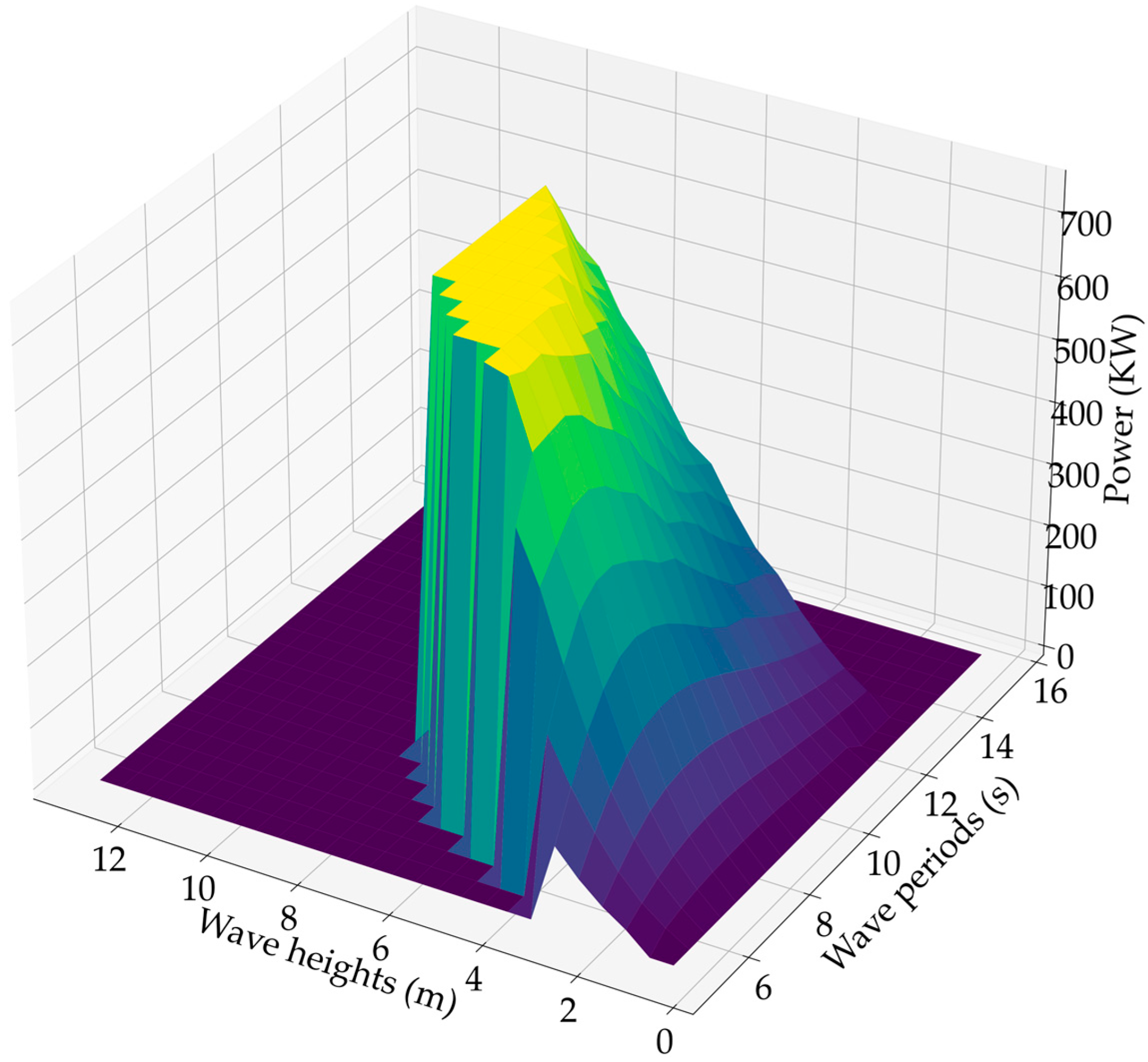
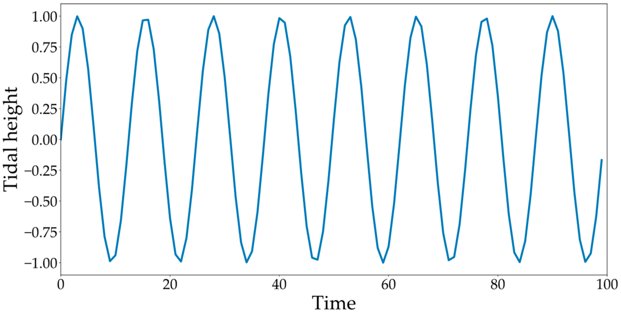
2.1. Wave Power Modelling

Similar to wind turbines’ power curves, the WEC has a power matrix model, often referred to as a wave power matrix (WPM). The WPM incorporates two essential variables: wave height and wave period. Through interpolation, it can determine the electrical power output of a WEC for any given wave parameter combination. Due to variations in the design of wave energy devices, their respective WPMs differ. Various types of WPMs are discussed in [15]. Each WEC is optimized to attain maximum power output at specific combinations of wave height and wave period, resulting in distinct operational frequencies and wave periods for individual WECs. Depending on environmental conditions, the operational states of a WEC can be categorized as follows: (1) before cut-in for power absorption capability limitation, (2) operating, and (3) cut-out for safety. A study conducted by A. Babarit [16] investigated eight different working principles of WECs and found significant similarities among these devices. Their performance indicators were in the same order of magnitude, approximately 1. The annual absorbed energy per root mean square of the power take-off (PTO) force was estimated to be around 2 MWh/kN.

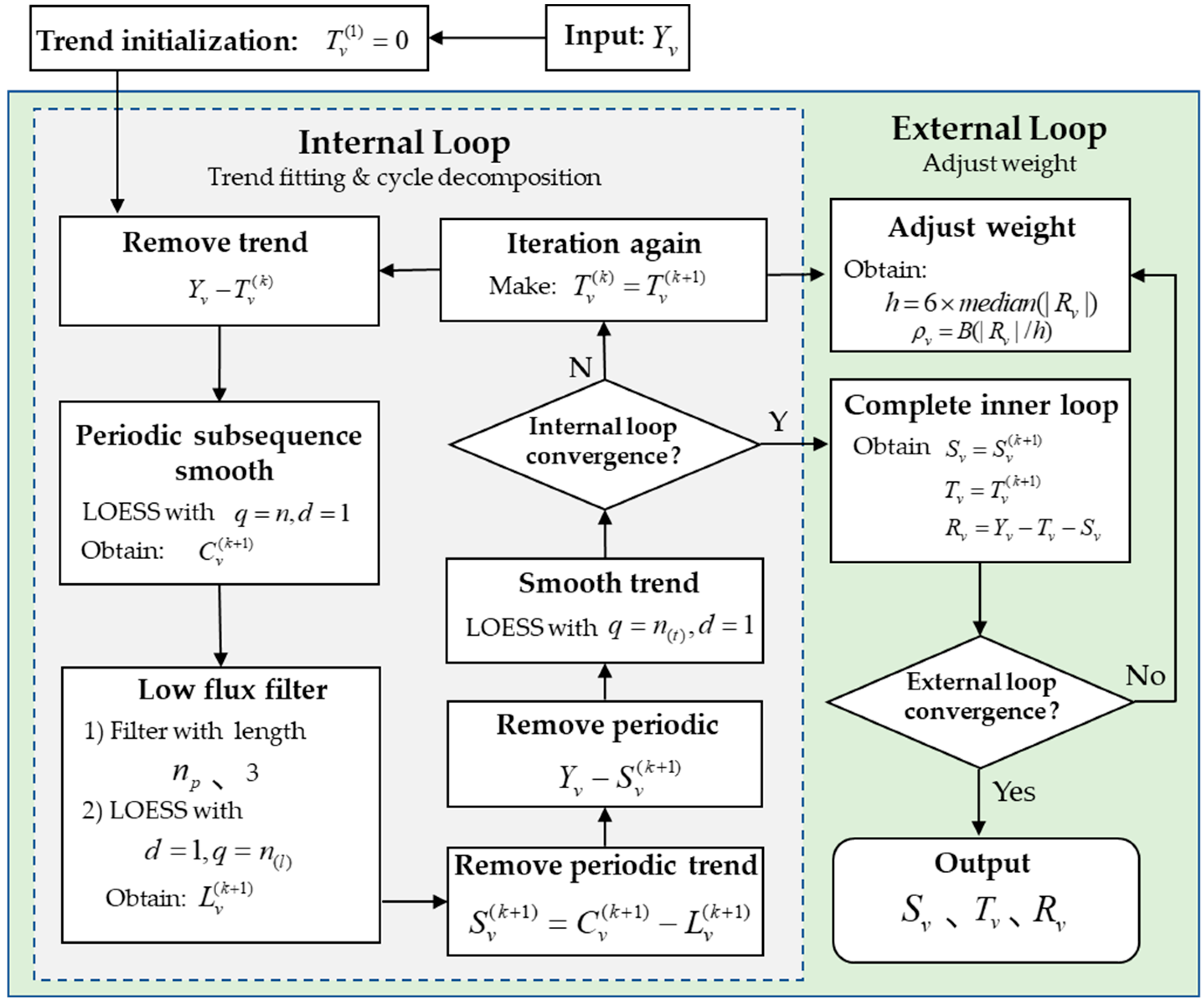
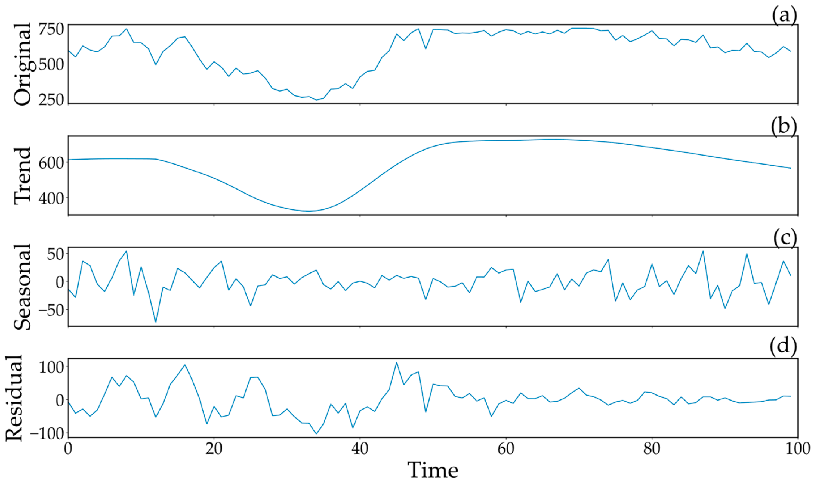
2.2. Seasonal–Trend Decomposition Using LOESS

Locally weighted scatterplot smoothing (LOESS) is a non-parametric, locally weighted smoothing method utilized for data smoothing. It accomplishes this by fitting a low-degree polynomial in proximity to each data point. STL [17] is a time series decomposition technique employed to break down time series data into three primary components: seasonal, trend, and residual components. The seasonal component represents the periodic patterns within the time series. STL has gained widespread application and has garnered significant recognition and success across various fields [18,19].
The decomposition process of STL comprises both an internal and an external loop. The internal loop refers to the stage where the original time series data are decomposed into low-frequency components such as trend and seasonality. Within the internal loop, the LOESS method is employed to fit the seasonal and trend components, providing a smoothed estimate of the original data. The outcome of this stage is a preliminary decomposition of seasonality and trend, wherein noise and high-frequency fluctuations persist. In contrast, the external loop encompasses a more intricate decomposition of high-frequency components, including residuals. This is based on the preliminary seasonal and trend components obtained from the internal loop. In the external loop, further smoothing is applied to the previously acquired seasonal and trend components, resulting in a more precise estimate of high-frequency fluctuations. This step produces a more accurate residual component, housing high-frequency noise and fluctuations unexplained by seasonality and trend.
To summarize, the STL method’s internal and external loops collaborate to address the low-frequency and high-frequency components of time series data, respectively. The STL method effectively decomposes time series data, capturing variations at different scales, including seasonality, trend, and residual components. The specific decomposition process is illustrated in Figure 1.

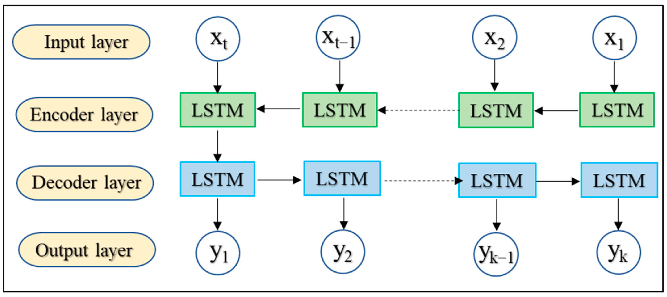
2.3. Seq2Seq Based on LSTM

LSTM is a deep learning model widely used for modelling and predicting sequential data. LSTM was first introduced by Hochreiter and Schmidhuber in 1997 [20]. Serving as an extension of recurrent neural networks (RNNs), LSTM was specifically designed to address the challenge of the vanishing gradient problem often encountered by RNNs when dealing with lengthy sequences. By incorporating gating mechanisms, LSTM can adaptively update its internal state, effectively capturing data variations across different time scales. This adaptability translates into exceptional performance when dealing with diverse time series data. LSTM has shown remarkable efficacy in various domains, including natural language processing [21], time series analysis [22], and computer vision [23]. Figure 2 illustrates the structure of an LSTM unit at time t. Its formal expression is provided in Table 1.
In the equations provided, σ represents the sigmoid function. W x i , W h i , and b i denote the weight matrices and bias vectors for the input gate. W x f , W h f , and b f represent the weight matrices and bias vectors for the forget gate. W x c , W h c , and b c stand for the weight matrices and bias vector for the cell state. W x o , W h o , and b o indicate the weight matrices and bias vectors for the output gate. represents element-wise multiplication.
The sequence-to-sequence (Seq2Seq) architecture was first introduced by Ilya Sutskever et al. [24]. This architecture was initially designed to address translation tasks in natural language processing and is now widely used in time series forecasting [25,26,27]. As illustrated in Figure 3, it begins by taking a sequence as input and then utilizes an encoder to generate a vector. This vector encapsulates the hidden information of the original sequence. Subsequently, the decoder is employed to decode this vector into a vector of the desired length.

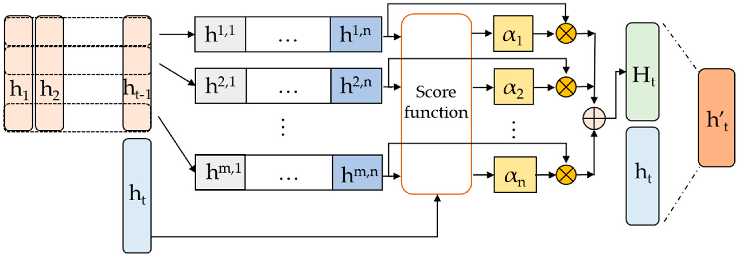
2.4. Temporal Pattern Attention

Temporal pattern attention (TPA) is a novel attention mechanism proposed by Shun-Yao Shih [28]. In contrast to conventional attention mechanisms that usually focus solely on information from the current time step to determine relevance, TPA is tailored for the prediction of diverse time series data. It enables attention to span across feature dimensions, distinguishing it from traditional mechanisms. The structure of TPA is shown in Figure 4.
TPA initially applies convolution to t − 1 hidden vectors from LSTM, where k convolution kernels can be set, and the convolution window w is often set to the total number of time steps. This operation can be formulated as follows:
H i , j = k = 1 w h i , ( t w 1 + k ) × C j , T w + l
In this equation, H i , j signifies the convolution result obtained by convolving the j-th convolution kernel with the i-th hidden vector in the feature dimension, while h i , ( t w 1 + k ) represents the hidden vectors subjected to convolution and C j , T w + l is the j-th filter.
α i = s i g m o i d ( ( H i ) T W a h t
The TPA weight calculation layer performs weighted operations on the convolution results and the last hidden vector h t from the LSTM encoder. The weight for the i-th hidden vector is represented as α i . W a is the weight matrix.
h t = W h h t + W v i = 1 n α i H i
h t represents the ultimate output of TPA, achieved by concatenating and summing the last hidden layer vector with the weighted hidden layer vectors. Both W h and W v are weight matrices.

2.5. Multi-Head Self-Attention

The multi-head self-attention mechanism was first introduced by Vaswani et al. in their seminal 2017 paper titled “Attention Is All You Need” [29]. It serves as a core component of the Transformer model. Periodic recurring information often encompasses long-term dependencies, necessitating the consideration of correlations spanning multiple time steps. The multi-head mechanism of self-attention allows the model to simultaneously learn multiple distinct attention weights. This capability enables the model to capture intricate relationships between different time steps and to discern periodic patterns of varying lengths [30].
For the calculation process of the i-th multi-head self-attention, the formulation is as follows:
Compute the linear transformations for Query (Q), Key (K), and Value (V):
Q i = Q × W Q i K i = K × W K i V i = V × W V i
where W Q i , W K i , and W V i are weight matrices used for linear transformations.
Calculate the attention scores:
A t t e n t i o n S c o r e ( Q i , K i ) = Q i × ( K i ) T
Perform scaling and Softmax operation:
A t t e n t i o n W e i g h t Q i ,   K i = S o f t m a x A t t e n t i o n S c o r e Q i ,   K i / d k
where d k represents the dimension of the key vectors.
Compute the output for each head:
H e a d i = A t t e n t i o n W e i g h t Q i ,   K i × V i
Concatenate the outputs from all heads and obtain the final multi-head self-attention output through a linear transformation:
M u l t i H e a d O u t p u t = c o n c a t H e a d 1 ,   H e a d 2 ,   ,   H e a d h × W O
where W O represents the weight matrix used for the final linear transformation.

2.6. Performance Evaluation

To validate the effectiveness of the model proposed in this paper, a comparative analysis is conducted using the following three evaluation metrics.
Root mean absolute error (RMSE):
R M S E = 1 n i = 1 n ( y i y ^ i ) 2 c a p
Mean absolute error (MAE):
M A E = 1 n i = 1 n | y i y ^ i | c a p
Determination coefficient (R2):
R 2 = 1 i = 1 n ( y i y ^ i ) 2 i = 1 n ( y i y ¯ ) 2
where y i and y ^ i represent the actual and predicted values at time i, and y ¯ represents the mean of the actual values. N is the length of the time series, and cap is the rated capacity of the wave energy converter.

3. Composition of the Proposed Model

In current wave power forecasting, modal decomposition methods like EWT are employed to process the model’s inputs, enhancing the model’s ability to extract fine-grained details. Modal decomposition excels at extracting periodic information from different modes. Physical processes at specific scales exhibit dominant periodic characteristics, and modal decomposition methods can introduce components without physical significance when applied across all scales. Moreover, an excessive number of components can burden the feature extraction process of the prediction model.
In this study, we employ STL to extract a trend sequence and dominant periodic seasonal sequence. To capture both large-scale trend information and efficiently extract primary periodic information and small fluctuations from seasonal sequences, we propose a dual-channel Seq2Seq prediction model. The wave power prediction process based on STL and the dual-channel Seq2Seq model can be summarized as follows:
Step 1: Conduct STL decomposition guided by the tidal period and the principle of maximum correlation to extract trend and seasonal sequences.
Step 2: Utilize the dual-channel Seq2Seq model to derive predictive results.

3.1. Determination of STL Decomposition Parameters

When conducting STL, it is essential to determine the decomposition period and window width. The selection of the decomposition period bears substantial physical significance and should be made in conjunction with the wave energy’s periodicity. Tide cycles introduce fluctuations in ocean water levels, exerting a discernible influence on the dynamics of wave propagation. During high tide, rising water levels tend to dampen wave propagation speeds, while during low tide, falling water levels can conversely accelerate wave propagation [31]. This intricate interplay can result in variations in wave amplitude and frequency. In light of these considerations, this study aligns the STL decomposition period with the tidal cycle, owing to its direct relevance to the behavior of waves.
The residual sequence encapsulates irregular fluctuations or noise that cannot be accounted for by the trend and seasonality components. Efforts are made to remove random noise from the residual sequence, making it closer to white noise, thus resulting in a cleaner and more meaningful decomposition outcome. The choice of the decomposition window width affects the effectiveness of STL decomposition. Here, a proposed method, as illustrated in Formula (12), is introduced. This method centers on the minimization of the autocorrelation within the residual sequence to determine the appropriate parameter.
w = arg min i = 1 i = n f ( i , w )
where w represents the optimal window width, and f ( i , w ) is the i-th order lag autocorrelation coefficient of the time series with a window width of w.

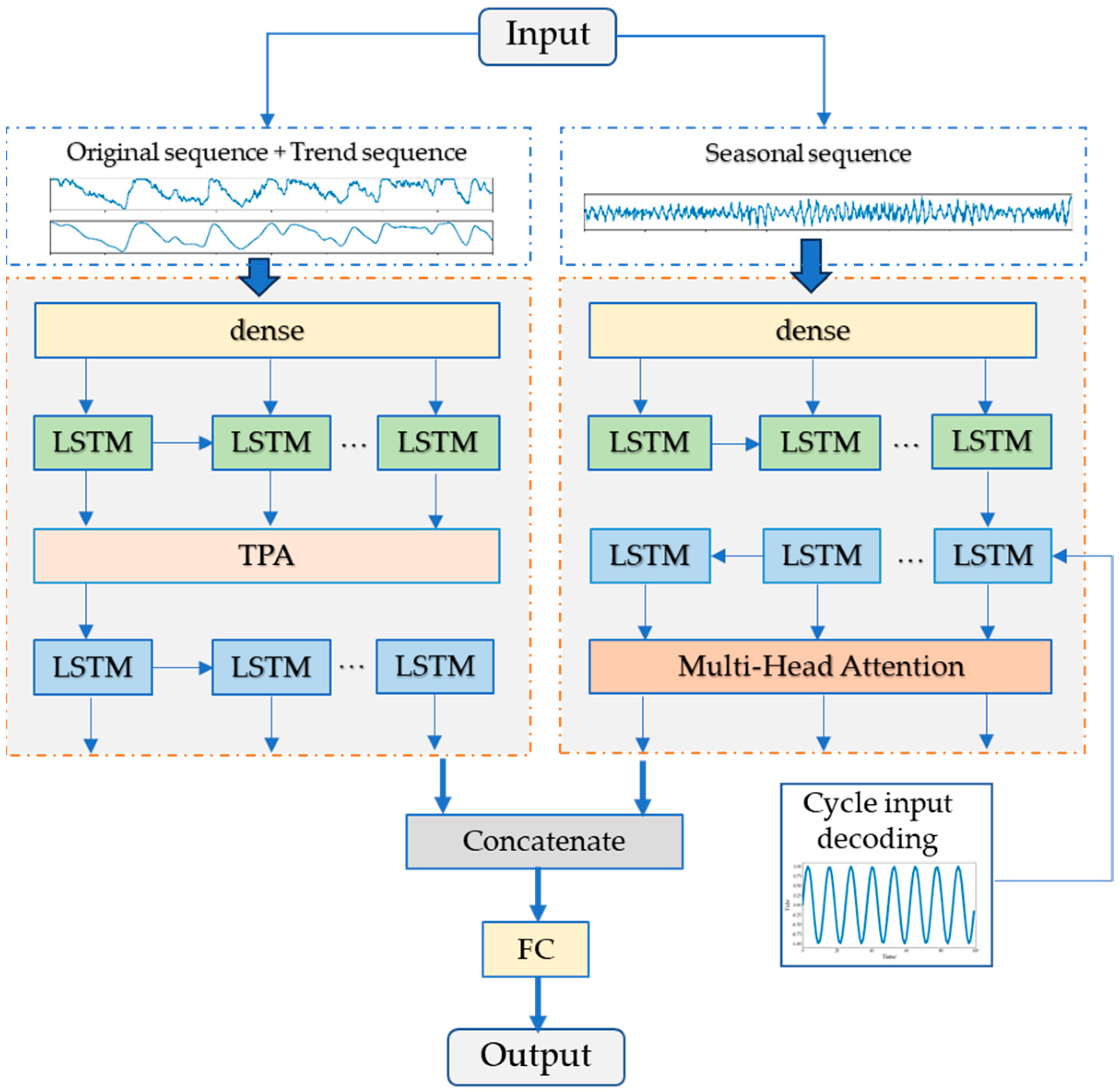
3.2. The Dual-Channel Seq2Seq Prediction Model

The proposed dual-channel Seq2Seq model is depicted in Figure 5. The Seq2Seq model comprises two distinct channels.
In the first channel, the input is constructed by concatenating the original sequence and the trend sequence across feature dimensions. The trend sequence exhibits relative smoothness and cannot capture other fluctuating information. Therefore, it is concatenated with the original sequence to create the input. Nevertheless, a simple concatenation of inputs could potentially compromise the model’s ability to extract trend features and impede its capacity to discern fine-grained features within the original sequence. To address this challenge, TPA is introduced after the Seq2Seq encoder. TPA conducts convolutions across feature dimensions, enabling it to explore distinctions and similarities among features. Its weighting module condenses the encoder’s features, and the resulting TPA-processed hidden layer vector serves as the initial state for the decoder. And a zero vector is used as the decoder’s input.
The second channel takes the seasonal component as its input, with the aim of enhancing the extraction of periodic features. An LSTM-based Seq2Seq is also used for encoding and decoding operations in this channel. To better extract periodic features from the sequence, a cosine sequence is generated based on the tidal cycle, and this cosine cycle sequence is used as the input for the decoder. By incorporating future tidal conditions into the decoder, the decoder can take into account forthcoming physical information, thereby providing more precise guidance for the model’s learning strategy. This approach enhances the accuracy of the model in predicting wave power and enables it to better adapt to dynamically changing environmental conditions. Then, the decoder’s output is processed through multi-head self-attention to weigh similar information, culminating in the final output of the second channel.
The outputs from both channels are concatenated, and a fully connected layer is used to produce the final prediction result.

4. Results and Discussion

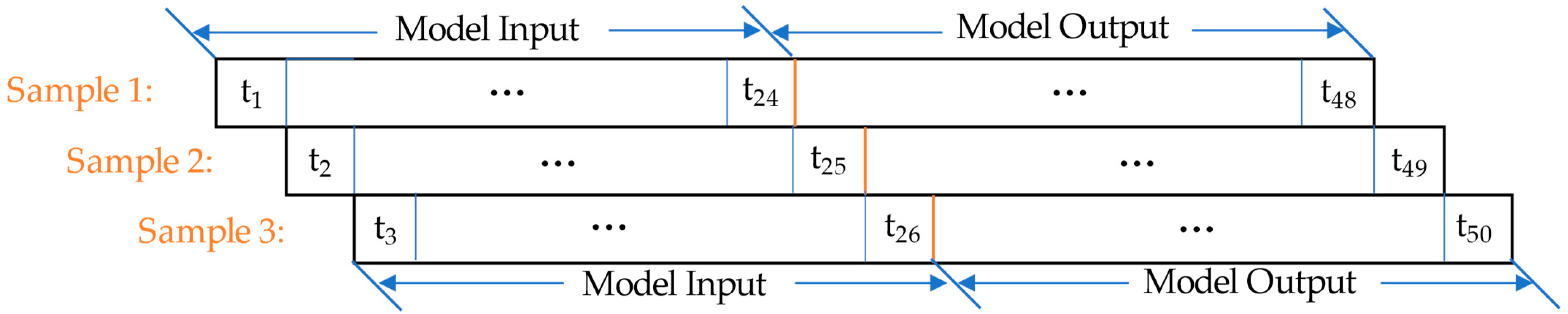
4.1. Data Preparation

The dataset employed in this investigation was sourced from the National Data Buoy Center, bearing the station identifiers 46001, situated at coordinates (56°18′1″ N, 148°1′6″ W), and 46029, at (46°9′48″ N, 124°29′12″ W). The temporal resolution of the two datasets is one hour. Within the dataset, an array of parameters is encompassed, including, but not limited to, wind velocity, wave amplitude, and wave frequency. Although these five years of data exhibit a semblance of completeness, it is pertinent to acknowledge the presence of occasional lacunae and spurious entries. For brief intervals of absent or erroneous data, the method of spline interpolation was judiciously employed to imbue continuity, whereas protracted periods of such data aberrations were judiciously omitted from the ensuing analysis.
The WPM selected for this study is “Pelamis”. This wave energy conversion device was utilized in the world’s first commercial wave energy project in Portugal during the year 2021. The relationship between wave height, wave period, and power is depicted in the 3D graph shown in Figure 6. Different colors indicate different power levels, with darker colors indicating lower power values.
For dataset 46001, the data spanning the years 2016, 2017, 2018, and 2020 are used for the training dataset, while the data for the year 2021 are used for the testing dataset. For dataset 46029, the data spanning the years 2015 to 2018 are the training dataset, and the year 2019 is the testing dataset. To facilitate model training and ensure uniform scaling among variables, this paper employs the min–max normalization technique.
X i = x i x min x max x min
Respectively, X i and x i represent the values prior to and subsequent to the normalization process, while x max and x min , respectively, denote the maximum and minimum values.
The model takes into account the power values observed over the preceding 24 h period as input and utilizes this information to forecast the power values for the ensuing 24 h. Samples are stratified utilizing a rolling window methodology, as exemplified in Figure 7. Consequently, a single value is simultaneously predicted in 24 different samples, each representing the predictive performance across various time intervals. This approach provides a larger dataset and facilitates the analysis of power prediction effectiveness across different time spans.

4.2. STL Results

The buoy’s behavior is predominantly subject to the semi-diurnal tide, with an approximate period of 12 h and 25 min [32]. Therefore, the chosen decomposition interval is set at 12 h. And the optimal window width is 5. In accordance with the suggested optimal decomposition criteria, both the training and testing datasets are independently subjected to decomposition. A selection of decomposition outcomes for the 2016 data in dataset 46001 is depicted in Figure 8.

4.3. Dual-Channel Seq2Seq Prediction

In the Seq2Seq model, the second channel employs cyclic decoding, as elucidated in Figure 9, conveying information about future tidal heights. The designated period is configured to be 12 h and 25 min. Grid search was employed for parameter optimization across all models, and key parameters for the proposed model are as follows: the first channel’s dense layer dimensions are (2, 48), encoder feature dimensions are (48, 128), and decoder dimensions are (128, 24); the second channel’s dense layer dimensions are (2, 30), encoder feature dimensions are (30, 96), and decoder dimensions are (96, 24). The fully connected output layer dimensions are (48, 24). The multi-head attention mechanism utilizes four heads.
Figure 10 portrays the forecasting outcomes for the test dataset at distinct time intervals, specifically at the 1st, 6th, 12th, and 24th time steps. The wave power exhibits diminished values during the mid-year period, juxtaposed with elevated values at the outset and conclusion of the entire year, delineating a conspicuous annual oscillation. On the whole, the proposed model yields satisfactory predictions, effectively tracking the multifarious patterns in wave power throughout the year. Notably, the forecast results at the sixth time step closely mirror the actual values, underscoring the model’s capacity to capture historical trends and undulations within the initial 6 h. While the predictions at the 24th time step exhibit a degree of temporal lag and may not precisely encapsulate the zenith and nadir of power values, they nonetheless succeed in encapsulating the overarching power trends.

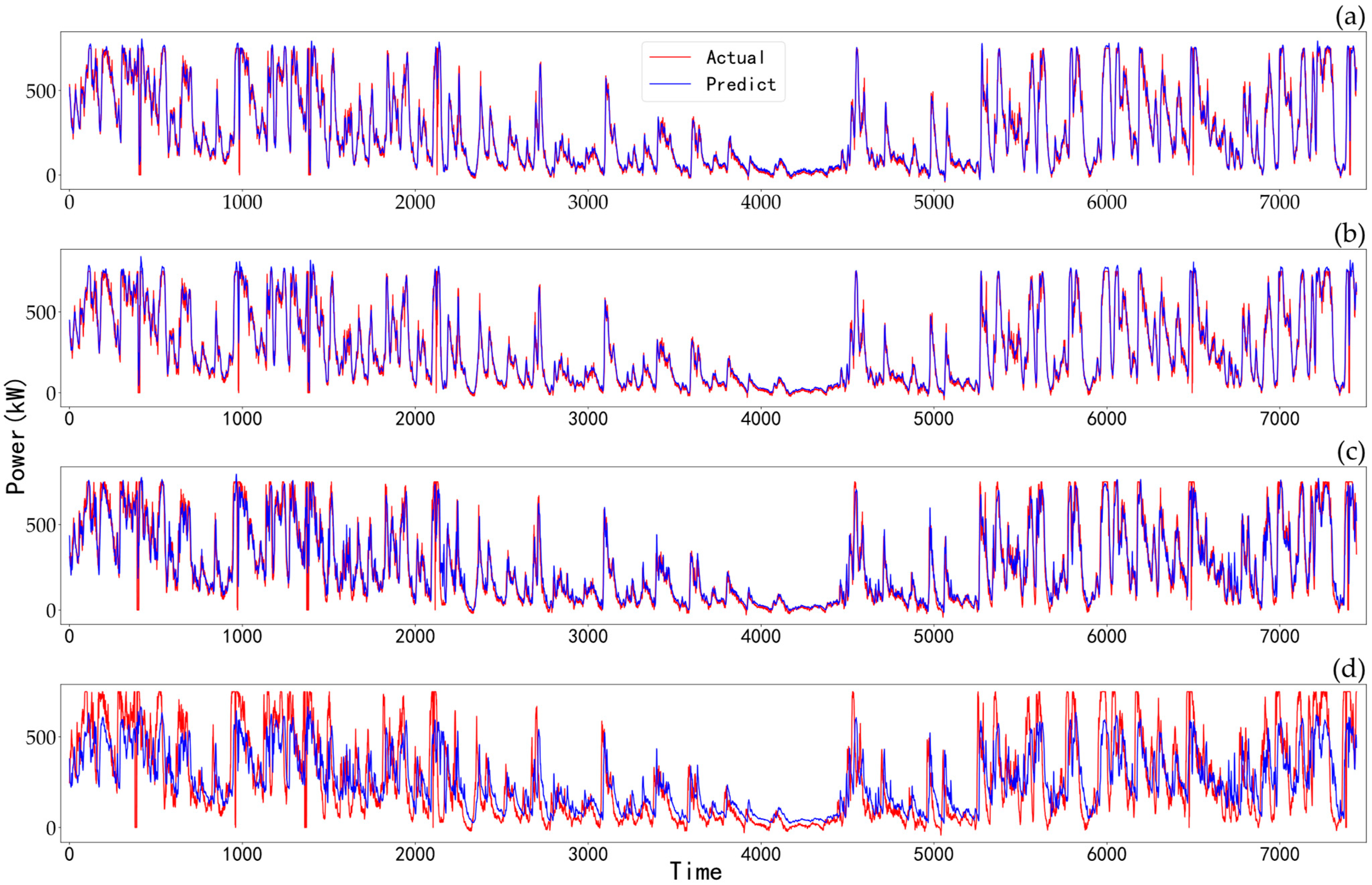
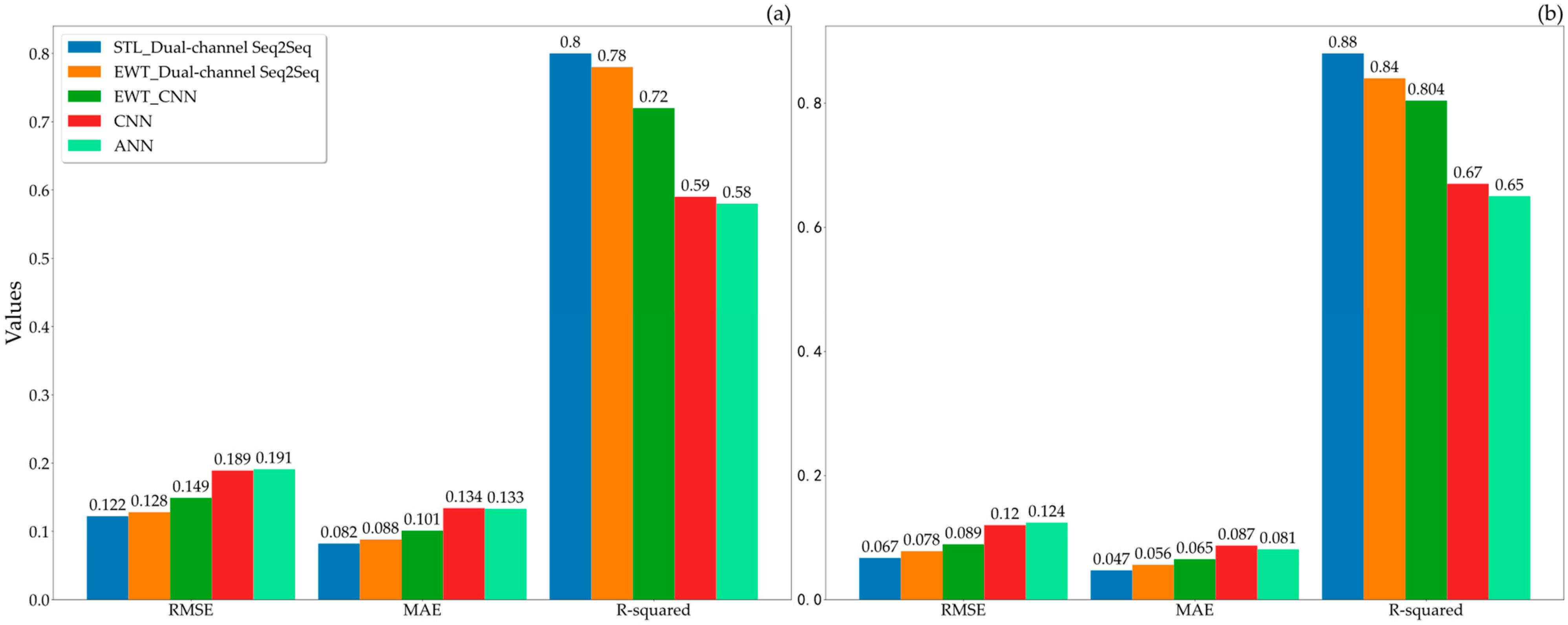
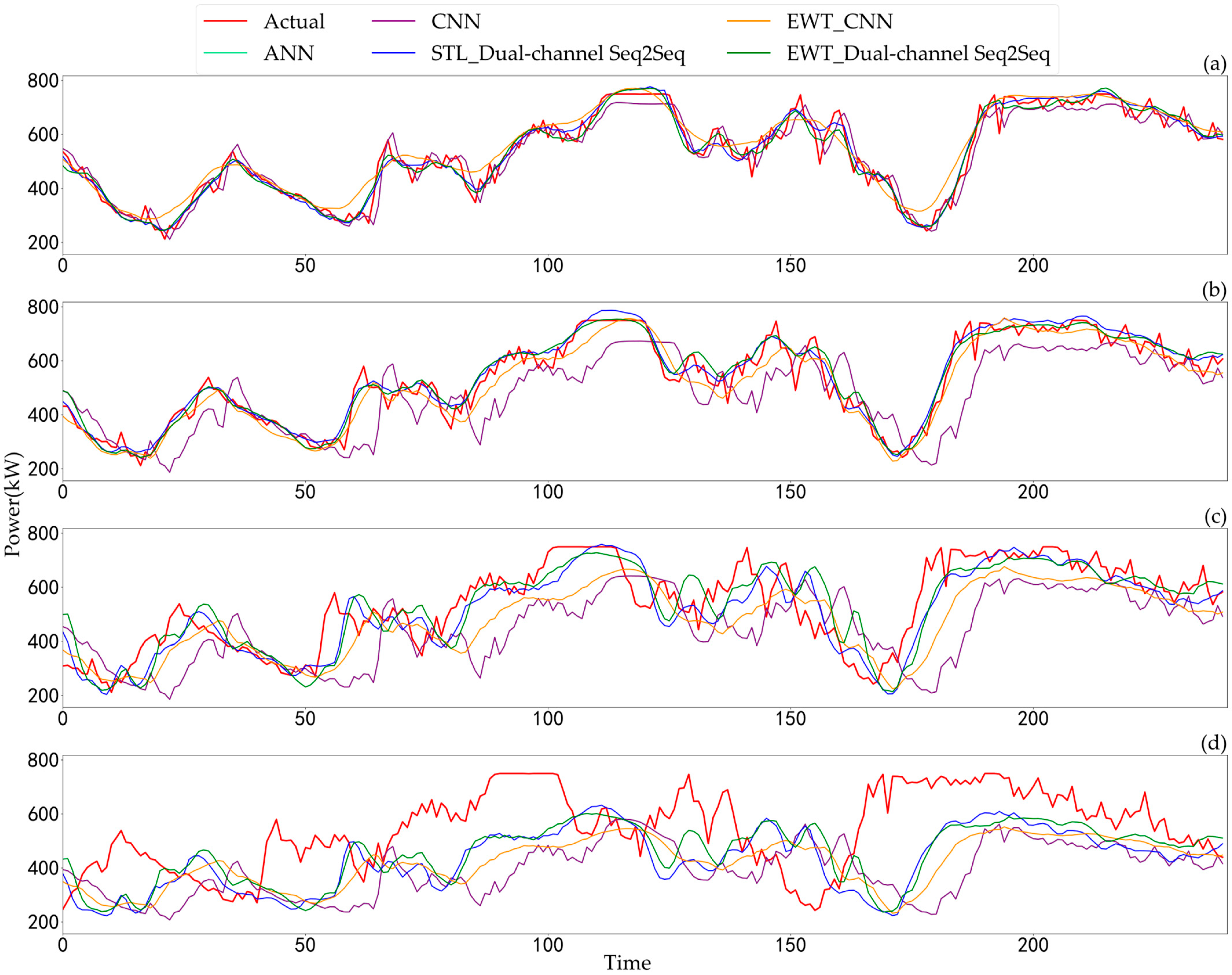
4.4. Comparison of Results

This study selected the baseline CNN and ANN model, EWT_CNN, and EWT_Dual-channel Seq2Seq as comparative models. The proposed model, which combines STL and dual-channel Seq2Seq, consistently yielded superior results.
To showcase the practical forecasting capabilities of the model for dataset 46001, Figure 11 presents the model’s predictions at various time horizons. With the increase in time steps, there is a noticeable trend of growing prediction errors across all models. This phenomenon arises due to the limited information inherent in historical data, leading to a diminishing predictive capacity over longer time spans. Subplots (a) and (b) display the predictions of all four models for the first and sixth time steps. Notably, all models except for the CNN and ANN perform admirably in tracking the actual values. Subplots (c) and (d) exhibit the model predictions for the twelfth and twenty-fourth time steps, where STL_Dual-channel Seq2Seq outperforms EWT_CNN in capturing longer-term trend features. Consequently, the decomposition of input data for prediction models proves effective in mitigating the escalation of prediction errors.
Table 2 provides a comprehensive view of the evaluation metrics for the four models across different prediction time steps. The proposed model consistently outperforms its counterparts at each time step. In contrast, the baseline model’s results exhibit linear-like trends in RMSE, MAE, and R-squared, with the lowest predictive accuracy among the comparative models. In contrast, the other three “decomposition-prediction” models show relatively stable RMSE and MAE trends in the early time steps, with errors starting to exhibit linear growth at a certain point. These models also demonstrate R-squared values that are relatively stable and close to 1 in the early time steps, with errors beginning to decrease linearly after a certain point. This observation underscores the capability of “decomposition-prediction” models to capture periodicity and maintain prediction accuracy within specific time intervals. And evaluation metrics of dataset 46029 in Appendix A show similar results.
Figure 12 presents the average evaluation metrics for all time steps for each model, with subplots (a) and (b) representing the results for dataset 46001 and dataset 46029, respectively. In dataset 46001, the proposed STL_Dual-channel Seq2Seq model outperforms the EWT_CNN model, demonstrating a reduction of 2.66% in RMSE and 1.86% in MAE. Furthermore, employing EWT_Dual-channel Seq2Seq over EWT_CNN leads to a 2.08% decrease in RMSE and a 1.29% reduction in MAE, highlighting the effectiveness of the proposed dual-channel Seq2Seq model. Additionally, STL_Dual-channel Seq2Seq outperforms EWT_Dual-channel Seq2Seq, achieving a further decrease of 0.58% in RMSE and 0.57% in MAE, emphasizing the superiority of the STL method over EWT. In comparison to the ANN, the CNN exhibits a slight advantage in the R2 metric, while yielding similar results in the other two metrics. The baseline model lags behind the ‘decomposition-prediction’ model overall. The magnitude of errors varies somewhat between the two datasets, with the proposed model still outperforming the EWT_CNN model by 2.2% in terms of RMSE for dataset 46029. This indicates the strong applicability of the proposed model.

5. Conclusions

This paper introduces an innovative wave power prediction model based on STL and dual-channel Seq2Seq architecture. A correlation-based optimal strategy is proposed to determine the decomposition window width, resulting in the best trend and seasonal components. Subsequently, a dual-channel Seq2Seq prediction model is designed. In the first channel, the TPA module is harnessed to extract features from the original sequence and trend component, thereby elucidating trend information and intricate details. The second channel employs multi-head self-attention and cyclic decoding to augment the extraction of periodic information from the seasonal component.
The performance of various models is evaluated and validated using five years of wave data from two buoys. The proposed model, along with other “decomposition-prediction” models, consistently exhibits lower errors compared to the baseline CNN model, confirming the effectiveness of the “decomposition-prediction” approach. Additionally, in dataset 46001, EWT_Dual-channel Seq2Seq outperforms EWT_CNN, achieving a reduction of 2.08% in RMSE and 1.29% in MAE, highlighting the effectiveness of the dual-channel Seq2Seq model. Furthermore, STL_Dual-channel Seq2Seq exhibits a further reduction of 0.58% in RMSE and 0.57% in MAE compared to EWT_Dual-channel Seq2Seq, demonstrating the efficacy of the STL method. The proposed model achieves an average 2.45% reduction in RMSE compared to EWT_CNN. The combination of STL and dual-channel Seq2Seq results in the highest prediction accuracy.
In summary, the proposed model excels in extracting periodic and trend features from historical information, thereby enhancing the accuracy of wave energy prediction. The current research solely utilizes wave energy power sequences for power prediction, without considering the influence of atmospheric physical mechanisms. Wave energy is affected by complex meteorological conditions such as wind speed and ocean currents. To enhance predictive accuracy for higher resolutions and longer forecast horizons, future research should analyze the impact of these factors. Both this study and current research predominantly employ theoretical power generation data for model training and prediction. When forecasting using actual wave energy generation data in the future, algorithms will also need to analyze the impact of the operational characteristics of different wave energy devices on the prediction outcomes.

Author Contributions

Z.L.: Conceptualization, Methodology. J.W.: Software, Writing—Original Draft. T.T.: Writing—Review and Editing, Supervision. Z.Z.: Writing—Review and Editing, Software. S.C.: Data Curation. Y.Y.: Supervision. S.H.: Writing—Original Draft. Y.L.: Writing—Review and Editing. All authors have read and agreed to the published version of the manuscript.

Funding

The work presented in this paper is part of the project “Research on Key Technologies for Megawatt-Level, High-Efficiency, and High-Reliability Wave Energy Power Generation Devices: Demonstration and Verification in the South China Sea Islands and Reefs” supported by the National Key Research and Development Program of China (No. 2019YFB1504404).

Data Availability Statement

The dataset utilized in this research is publicly available from the National Data Buoy Center at http://www.ndbc.noaa.gov (accessed on 7 November 2023).

Conflicts of Interest

The authors declare that they do not have any known competing interests that could have appeared to influence the work reported in this paper.

Appendix A

Table A1. Performance evaluation of prediction models of dataset 46029.
Time
Step
STL_Dual-Channel Seq2SeqEWT_Dual-Channel Seq2SeqEWT_CNNCNNANN
RMSE
(%)
MAE
(%)
R2RMSE
(%)
MAE
(%)
R2RMSE
(%)
MAE
(%)
R2RMSE
(%)
MAE
(%)
R2RMSE
(%)
MAE
(%)
R2
12.821.910.982.902.120.986.822.350.973.962.770.974.414.050.96
22.842.010.983.012.310.986.612.550.974.973.490.955.355.000.94
32.791.970.983.062.350.986.162.690.976.124.310.926.446.020.91
42.781.970.983.142.410.985.702.780.977.175.000.897.536.980.88
52.801.980.983.172.420.985.502.890.978.125.620.868.528.610.85
62.842.000.983.072.350.986.113.120.968.956.170.839.379.330.82
72.922.040.982.972.280.987.423.530.959.706.690.8110.1210.000.79
83.172.210.983.332.530.989.074.060.9310.377.210.7810.7810.880.76
93.412.410.984.243.160.9610.784.650.9110.967.670.7511.3511.520.73
103.682.610.975.313.860.9412.365.240.8911.518.100.7311.8812.700.71
114.413.120.966.334.530.9213.795.800.8612.038.530.7012.3813.780.68
125.223.720.947.305.160.8915.116.320.8312.518.950.6812.8614.180.66
136.094.380.928.185.780.8616.336.830.8112.969.360.6513.3114.430.63
146.824.950.908.986.330.8317.447.300.7813.429.740.6313.7715.110.61
157.575.520.889.716.840.8118.457.760.7613.8510.090.6014.2015.620.58
168.396.070.8510.397.330.7819.378.180.7314.2710.430.5814.6216.120.56
179.276.640.8211.047.810.7520.228.600.7114.6710.770.5615.0416.510.53
1810.147.190.7911.638.270.7220.999.000.6815.0511.100.5315.4317.060.51
1910.897.640.7612.198.700.6921.689.360.6615.4211.400.5115.8017.370.48
2011.487.990.7312.669.080.6722.309.700.6415.7611.690.4916.1618.230.46
2111.898.240.7113.079.420.6522.8710.040.6216.0911.960.4716.4918.230.44
2212.198.450.6921.909.740.6323.3910.360.6016.3912.220.4516.813.140.42
2312.548.740.6822.4510.040.6123.8610.700.5716.6812.460.4317.113.630.40
2412.879.050.6622.9510.340.5924.2911.030.5516.9412.690.4117.384.260.38

References

  1. Shadman, M.; Roldan-Carvajal, M.; Pierart, F.G.; Haim, P.A.; Alonso, R.; Silva, C.; Osorio, A.F.; Almonacid, N.; Carreras, G.; Maali Amiri, M.; et al. A Review of Offshore Renewable Energy in South America: Current Status and Future Perspectives. Sustainability 2023, 15, 1740. [Google Scholar] [CrossRef]
  2. Yan, J.; Mei, N.; Zhang, D.; Zhong, Y.; Wang, C. Review of Wave Power System Development and Research on Triboelectric Nano Power Systems. Front. Energy Res. 2022, 10, 966567. [Google Scholar] [CrossRef]
  3. Zhang, Y.; Zhao, Y.; Sun, W.; Li, J. Ocean Wave Energy Converters: Technical Principle, Device Realization, and Performance Evaluation. Renew. Sustain. Energy Rev. 2021, 141, 110764. [Google Scholar] [CrossRef]
  4. Clemente, D.; Rosa-Santos, P.; Taveira-Pinto, F. On the Potential Synergies and Applications of Wave Energy Converters: A Review. Renew. Sustain. Energy Rev. 2021, 135, 110162. [Google Scholar] [CrossRef]
  5. Gao, Q.; Khan, S.S.; Sergiienko, N.; Ertugrul, N.; Hemer, M.; Negnevitsky, M.; Ding, B. Assessment of Wind and Wave Power Characteristic and Potential for Hybrid Exploration in Australia. Renew. Sustain. Energy Rev. 2022, 168, 112747. [Google Scholar] [CrossRef]
  6. Sun, R.; Cobb, A.; Villas Bôas, A.B.; Langodan, S.; Subramanian, A.C.; Mazloff, M.R.; Cornuelle, B.D.; Miller, A.J.; Pathak, R.; Hoteit, I. Waves in SKRIPS: WAVEWATCH III Coupling Implementation and a Case Study of Tropical Cyclone Mekunu. Geosci. Model Dev. 2023, 16, 3435–3458. [Google Scholar] [CrossRef]
  7. Amarouche, K.; Akpınar, A.; Rybalko, A.; Myslenkov, S. Assessment of SWAN and WAVEWATCH-III Models Regarding the Directional Wave Spectra Estimates Based on Eastern Black Sea Measurements. Ocean. Eng. 2023, 272, 113944. [Google Scholar] [CrossRef]
  8. Wu, F.; Jing, R.; Zhang, X.-P.; Wang, F.; Bao, Y. A Combined Method of Improved Grey BP Neural Network and MEEMD-ARIMA for Day-Ahead Wave Energy Forecast. IEEE Trans. Sustain. Energy 2021, 12, 2404–2412. [Google Scholar] [CrossRef]
  9. Guillou, N. Estimating Wave Energy Flux from Significant Wave Height and Peak Period. Renew. Energy 2020, 155, 1383–1393. [Google Scholar] [CrossRef]
  10. Ni, C. Data-driven Models for Short-term Ocean Wave Power Forecasting. IET Renew. Power Gen 2021, 15, 2228–2236. [Google Scholar] [CrossRef]
  11. Ni, C.; Ma, X. Prediction of Wave Power Generation Using a Convolutional Neural Network with Multiple Inputs. Energies 2018, 11, 2097. [Google Scholar] [CrossRef]
  12. Lu, H.; Xi, D.; Ma, X.; Zheng, S.; Huang, C.; Wei, N. Hybrid Machine Learning Models for Predicting Short-Term Wave Energy Flux. Ocean. Eng. 2022, 264, 112258. [Google Scholar] [CrossRef]
  13. Gómez-Orellana, A.M.; Guijo-Rubio, D.; Gutiérrez, P.A.; Hervás-Martínez, C. Simultaneous Short-Term Significant Wave Height and Energy Flux Prediction Using Zonal Multi-Task Evolutionary Artificial Neural Networks. Renew. Energy 2022, 184, 975–989. [Google Scholar] [CrossRef]
  14. Ni, C.; Peng, W. An Integrated Approach Using Empirical Wavelet Transform and a Convolutional Neural Network for Wave Power Prediction. Ocean. Eng. 2023, 276, 114231. [Google Scholar] [CrossRef]
  15. Rasool, S.; Muttaqi, K.M.; Sutanto, D.; Hemer, M. Quantifying the Reduction in Power Variability of Co-Located Offshore Wind-Wave Farms. Renew. Energy 2022, 185, 1018–1033. [Google Scholar] [CrossRef]
  16. Babarit, A.; Hals, J.; Muliawan, M.J.; Kurniawan, A.; Moan, T.; Krokstad, J. Numerical Benchmarking Study of a Selection of Wave Energy Converters. Renew. Energy 2012, 41, 44–63. [Google Scholar] [CrossRef]
  17. Cleveland, R.B.; Cleveland, W.S. STL: A Seasonal-Trend Decomposition Procedure Based on Loess. J. Off. Stat. 1990, 6, 3–33. [Google Scholar]
  18. Li, W.; Jiang, X. Prediction of Air Pollutant Concentrations Based on TCN-BiLSTM-DMAttention with STL Decomposition. Sci. Rep. 2023, 13, 4665. [Google Scholar] [CrossRef]
  19. Stefenon, S.F.; Seman, L.O.; Mariani, V.C.; Coelho, L.D.S. Aggregating Prophet and Seasonal Trend Decomposition for Time Series Forecasting of Italian Electricity Spot Prices. Energies 2023, 16, 1371. [Google Scholar] [CrossRef]
  20. Hochreiter, S.; Schmidhuber, J. Long Short-Term Memory. Neural Comput. 1997, 9, 1735–1780. [Google Scholar] [CrossRef]
  21. Wei, W.; Li, X.; Zhang, B.; Li, L.; Damaševičius, R.; Scherer, R. LSTM-SN: Complex Text Classifying with LSTM Fusion Social Network. J. Supercomput. 2023, 79, 9558–9583. [Google Scholar] [CrossRef]
  22. Chen, H.; Lu, T.; Huang, J.; He, X.; Yu, K.; Sun, X.; Ma, X.; Huang, Z. An Improved VMD-LSTM Model for Time-Varying GNSS Time Series Prediction with Temporally Correlated Noise. Remote Sens. 2023, 15, 3694. [Google Scholar] [CrossRef]
  23. Harie, Y.; Gautam, B.P.; Wasaki, K. Computer Vision Techniques for Growth Prediction: A Prisma-Based Systematic Literature Review. Appl. Sci. 2023, 13, 5335. [Google Scholar] [CrossRef]
  24. Sutskever, I.; Vinyals, O.; Le, Q.V. Sequence to Sequence Learning with Neural Networks. Adv. Neural Inf. Process. Syst. 2014, 27, 3104–3112. [Google Scholar]
  25. Dong, H.; Zhu, J.; Li, S.; Wu, W.; Zhu, H.; Fan, J. Short-Term Residential Household Reactive Power Forecasting Considering Active Power Demand via Deep Transformer Sequence-to-Sequence Networks. Appl. Energy 2023, 329, 120281. [Google Scholar] [CrossRef]
  26. Yang, M.; Wang, D.; Zhang, W. A Short-Term Wind Power Prediction Method Based on Dynamic and Static Feature Fusion Mining. Energy 2023, 280, 128226. [Google Scholar] [CrossRef]
  27. Qian, C.; Xu, B.; Xia, Q.; Ren, Y.; Sun, B.; Wang, Z. SOH Prediction for Lithium-Ion Batteries by Using Historical State and Future Load Information with an AM-Seq2seq Model. Appl. Energy 2023, 336, 120793. [Google Scholar] [CrossRef]
  28. Shih, S.-Y.; Sun, F.-K.; Lee, H. Temporal Pattern Attention for Multivariate Time Series Forecasting. Mach. Learn. 2019, 108, 1421–1441. [Google Scholar] [CrossRef]
  29. Vaswani, A.; Shazeer, N.; Parmar, N.; Uszkoreit, J.; Jones, L.; Gomez, A.N.; Kaiser, L.; Polosukhin, I. Attention Is All You Need. Adv. Neural Inf. Process. Syst. 2017, 30, 5998–6008. [Google Scholar]
  30. Wang, X.; Li, Y.; Xu, Y.; Liu, X.; Zheng, T.; Zheng, B. Remaining Useful Life Prediction for Aero-Engines Using a Time-Enhanced Multi-Head Self-Attention Model. Aerospace 2023, 10, 80. [Google Scholar] [CrossRef]
  31. Phan, H.M.; Ye, Q.; Reniers, A.J.H.M.; Stive, M.J.F. Tidal Wave Propagation along The Mekong Deltaic Coast. Estuar. Coast. Shelf Sci. 2019, 220, 73–98. [Google Scholar] [CrossRef]
  32. Ray, R.D. First Global Observations of Third-Degree Ocean Tides. Sci. Adv. 2020, 6, eabd4744. [Google Scholar] [CrossRef] [PubMed]
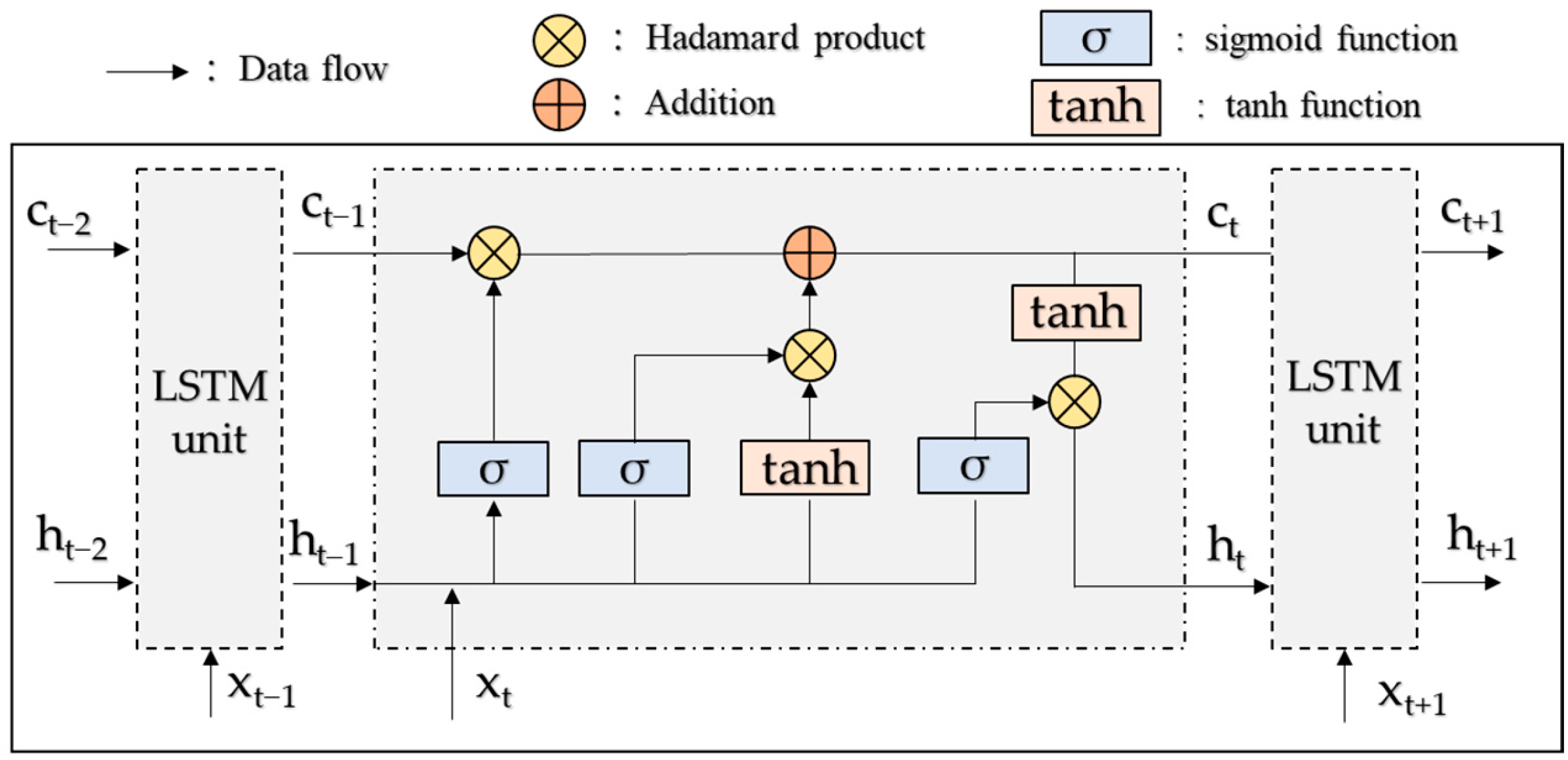
Figure 1. STL analysis algorithm flow. “Y” means “Yes”. “N” means “No”.
Energies 16 07515 g001
Figure 2. Structure of LSTM networks.
Energies 16 07515 g002
Figure 3. Structure of Seq2Seq model.
Energies 16 07515 g003
Figure 4. Structure of TPA.
Energies 16 07515 g004
Figure 5. Structure of dual-channel Seq2Seq model.
Energies 16 07515 g005
Figure 6. Power matrix of “Pelamis”.
Energies 16 07515 g006
Figure 7. Method of sample splitting.
Energies 16 07515 g007
Figure 8. Decomposition of power sequence of (a) original sequence, (b) trend sequence, (c) seasonal sequence, and (d) residual sequence.
Energies 16 07515 g008
Figure 9. Cyclic input of decoder.
Energies 16 07515 g009
Figure 10. Predictions of the proposed model for lead times of (a) 1 h, (b) 6 h, (c) 12 h, and (d) 24 h in dataset 46001.
Energies 16 07515 g010
Figure 11. Predictions of models for lead times of (a) 1 h, (b) 6 h, (c) 12 h, and (d) 24 h in dataset 46001.
Energies 16 07515 g011
Figure 12. Average prediction errors of all time steps of (a) dataset 46001 and (b) dataset 46029.
Energies 16 07515 g012
Table 1. LSTM computational formula.
LSTM StructureExpression Formula
Input gate i t = σ ( W x i · x t + W h i · h t 1 + b i )
Forget gate f t = σ ( W x f · x t + W h f · h t 1 + b f )
Cell gate c ˜ t = t a n h ( W x c · x t + W h c · h t 1 + b c )
Output gate o t = σ ( W x o · x t + W h o · h t 1 + b o )
Cell state c t = f t c t 1 + i t c ˜ t
Hidden state h t = o t t a n h ( c t )
Table 2. Performance evaluation of prediction models.
Time
Step
STL_Dual-Channel Seq2SeqEWT_Dual-Channel Seq2SeqEWT_CNNCNNANN
RMSE
(%)
MAE
(%)
R2RMSE
(%)
MAE
(%)
R2RMSE
(%)
MAE
(%)
R2RMSE
(%)
MAE
(%)
R2RMSE
(%)
MAE
(%)
R2
14.963.010.975.103.030.976.824.120.956.754.050.956.794.050.95
24.882.990.975.153.160.976.613.910.958.295.030.938.315.000.92
34.863.050.985.053.120.976.163.750.9610.036.220.8910.066.020.88
45.003.100.975.083.150.975.703.540.9711.637.380.8611.686.980.86
55.053.190.975.113.190.975.503.370.9713.158.510.8213.258.610.81
65.053.190.975.103.210.976.113.620.9614.479.530.7814.479.330.77
74.883.010.975.223.170.977.424.430.9415.6510.460.7415.7210.000.73
85.253.120.976.003.600.969.075.490.9116.6811.290.7116.6910.880.70
96.633.940.957.494.520.9410.786.640.8817.6112.020.6717.5911.520.67
108.265.000.939.125.610.9112.367.740.8418.4912.700.6418.4512.700.63
119.806.060.9010.636.670.8813.798.780.8019.3013.360.6119.3713.780.59
1211.297.100.8712.037.740.8515.119.770.7620.0614.030.5820.0514.180.57
1312.668.120.8313.328.760.8116.3310.730.7220.7614.600.5520.8014.430.54
1413.889.070.8014.499.730.7817.4411.630.6821.4415.190.5221.5215.110.51
1515.009.970.7615.6010.640.7418.4512.480.6422.0715.770.4922.1815.620.48
1616.0310.800.7316.6811.540.7119.3713.270.6122.6616.320.4622.5416.120.45
1717.0111.590.7017.7712.430.6720.2214.000.5723.1716.810.4423.1516.510.44
1817.9812.390.6618.8013.280.6320.9914.670.5423.6217.260.4123.7317.060.41
1918.9513.180.6219.7514.090.5921.6815.310.5124.0317.670.3924.3317.370.39
2019.8113.890.5920.5814.840.5622.3015.900.4824.3918.030.3824.5318.230.36
2120.5214.490.5621.2815.500.5222.8716.450.4524.6918.330.3624.9218.230.35
2221.1415.050.5321.9016.130.5023.3916.960.4324.9518.610.3525.3618.210.33
2321.7015.570.5122.4516.720.4723.8617.430.4025.1818.830.3425.9119.130.32
2422.2216.090.4822.9517.290.4524.2917.860.3825.4219.070.3226.2219.240.30
Disclaimer/Publisher’s Note: The statements, opinions and data contained in all publications are solely those of the individual author(s) and contributor(s) and not of MDPI and/or the editor(s). MDPI and/or the editor(s) disclaim responsibility for any injury to people or property resulting from any ideas, methods, instructions or products referred to in the content.

