Abstract
The Dual–Vector model predictive control (DV–MPC) method can improve the steady–state control performance of motor drives compared to using the single–vector method in one switching cycle. However, this performance enhancement generally increases the computational burden due to the exponential increase in the number of vector selections, lowering the system’s dynamic response. Alternatively, limiting the vector combinations will sacrifice system steady–state performance. To address this issue, this paper proposes an enhanced DV–MPC method that can determine the optimal vector combinations along with their duration time within minimized calculation times. Compared to the existing DV–MPC methods, the proposed enhanced technique can achieve excellent steady–state performance while maintaining a low computational burden. These benefits have been demonstrated in the results from a 2.5k rpm permanent magnet synchronous motor drive.
1. Introduction
The permanent magnet synchronous motor (PMSM) has been widely used in transportation applications due to its high power density and efficiency [1,2]. For a PMSM drive system, excellent dynamic performance is desirable, especially for variable–speed motor drive applications. Thus, model predictive control (MPC) techniques with rapid responses have gained interest in the PMSM drive control [3,4,5,6].
However, the traditional single–vector MPC (SV–MPC) technique applies only one voltage vector in every switching cycle, resulting in poor control performance [7,8]. To address this issue, researchers have proposed a Dual–Vector MPC (DV–MPC) technique that applies two voltage vectors within each switching cycle [9,10]. Despite achieving an improved control performance when using the DV–MPC method, more vectors employed adversely increases the calculation burden. For a two–level inverter with seven available voltage space vectors, 49 calculation cycles are needed to determine the two optimal vectors [11]. To reduce the computational burden of the DV–MPC technique, [12,13,14,15,16] suggest excluding the redundant and replaceable vector combinations, which can cut the number of computation cycles from 49 to 25.
Instead of searching for the two arbitrary vectors, adopting adjacent space vectors can effectively improve the processing speed of the DV–MPC technique [12,13,14,15,16]. To begin with, the vector selection can be confined by one active vector and one zero vector. For example, in [12], the optimal vector combination is selected among the six combinations obtained through combining the six active vectors with the zero vector. In [13], the selection of the first vector is fixed to the active vector applied in the previous sampling period and its adjacent active vectors, which can reduce the computation cycles to three [13]. However, the composed vector of one active and one zero vector in [12,13] can only lie on the active vectors, which can lead to an undesirable output ripple.
Alternatively, another vector selection method can be implemented by locating the reference vector from its angle to the reference vector. Then, the two vectors that are closest to the reference vector among the three vectors (two active vectors and one zero vector) contained in that sector are selected [14,15]. In [16], after determining the vector nearest to the reference vector, the second applied vector is fixed to be either the neighboring vector of the first vector or the zero vector. Those methods [14,15,16] can save the computational burden compared to using the DV–MPC method [11], but their vector synthetic range is limited to the active vectors themselves or the boundaries of the space vector diagram, affecting the control performance.
In this paper, the limitations imposed by using only the adjacent vectors are analyzed and explained. This is followed by proposing the improved DV–MPC method considering all available vector combinations. This paper has proven that only five prediction times are needed to determine the optimal vector combination. In addition, the information on the projections among vectors can be applied to determining the sector of the reference vector without the need for trigonometric functions. To summarize, the main contributions of this paper include:
- Analyzing the limitation of using adjacent vectors as seen in the existing DV–MPC methods in the literature.
- Proposing an enhanced DV–MPC technique considering two arbitrary vector combinations with the improvement in terms of the steady–state as well as the dynamic control performance.
- Proposing a method to quickly determine the sector by only three calculations.
- To validate the effectiveness of the proposed method, it is compared with the existing SV–MPC method and the DV–MPC methods in the literature.
The rest of this paper is organized as follows. Section 2 briefly describes the principle of the DV–MPC method of employing the adjacent vectors in [14], and states explicitly its limitations. Section 3 introduces the proposed improved DV–MPC technique. Section 4 compares and validates this approach with other MPC methods in the following. Finally, conclusions are drawn in Section 5.
2. Dual–Vector MPC Principle and Its Limitation
The DV–MPC method mainly includes reference voltage vector acquisition, selection of the first and second vectors, and calculation of vector duration time. This section briefly introduces the DV–MPC method in [14] and discusses the limitation of adopting the adjacent vectors in detail.
2.1. Working Principle
Using the deadbeat control principle and forward Euler combined with the PMSM mathematical model, the relationship between the αβ− reference stator voltage uαref, uβref and the stator current iα, iβ can be expressed:
where ψf is permanent magnet flux linkage, Ls and R are stator inductance and winding resistance, ωe and θ are the angular velocity and rotor position angle, Ts is the sampling period, and k is the sampling moment.
The angle θref of the reference voltage vector can be obtained through (3). After that, the sector in which the reference vector is located can be determined.
After the sector is determined, the best vector combination is the two vectors Vm and Vn closest to the reference vector. Their respective duration tm, tn is obtained via solving the equations in (4):
2.2. Limitation Discussion
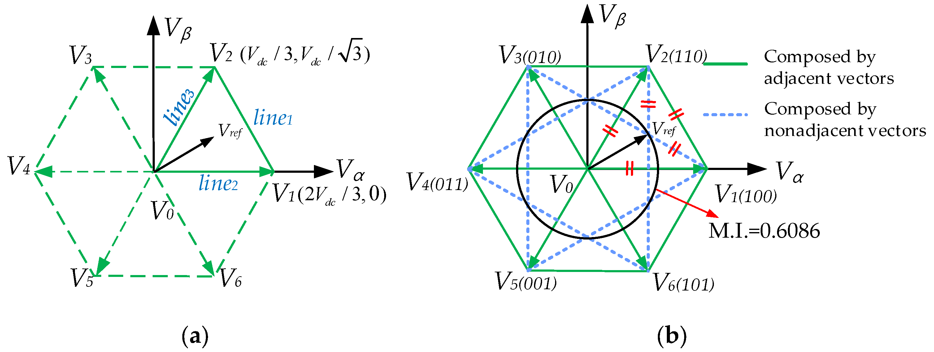
When using the adjacent vectors, the resultant vector uses only the active vectors and the boundary of the sector. For example, when the reference vector is in Sector I of the space vector diagram, the composition range by adjacent vectors of Sector I follows the straight lines as shown in Figure 1a:
where Line1, Line2, and Line3 are the synthetic region of (V1, V2), (V1, V0), and (V2, V0), respectively.
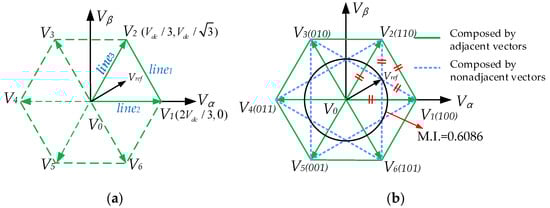
Figure 1.
Composed range using: (a) two adjacent vectors in Sector I; (b) two arbitrary vectors.
However, if nonadjacent effective vectors are also synthesized, all the possible synthetic regions are as shown in Figure 1b. It can be seen from Figure 1b that when the modulated index (M.I.) is at the middle range, such as around 0.6086, the vector synthesized by the nonadjacent active vector outperforms the vector synthesized by the adjacent active vector. This is because the vector synthesized using nonadjacent vectors is closer to the reference vector than the vector synthesized using adjacent vectors.
As shown in Figure 1b, there are five straight lines in each sector, which means that there are only five options for the vector combination in total. Therefore, after determining the sector in which the reference vector is located, only five prediction attempts are required to determine the optimal vector combination.
3. Proposed DV–MPC Technique
Through the analysis and discussion in Section 2.2, it can be concluded that the vector selection method in the previous section is not the optimal solution due to the limitations of the vectors synthesized by adjacent vectors. Therefore, a new DV–MPC method is proposed to extend the vector combination in the DV–MPC method in [14], and the specific steps will be discussed in this section.
3.1. Control Block Diagram of the Proposed Method
As shown in Figure 2, the control system for a PMSM can be driven by a two–level, three–phase voltage source inverter. The speed error obtained via the speed loop is adjusted by the PI controller to produce the q–axis current reference value iq*. The current coordinate system is then established in combination with the mathematical model of the PMSM and the seven possible switching states (see Section 3.2). Five sets of candidate vector combinations (Ci) can be determined by determining the sector where the reference current vector is located (see Table 1 and Table 2). Vector combinations can be selected and evaluated according to the corresponding cost function Gi (see Section 3.3 and Section 3.4). The vector duration is determined by the minimization of steady–state current error ess. Finally, at the next control cycle, the determined voltage vector corresponds to the inverter switch state and the corresponding duration, resulting in the control of motor rotation.
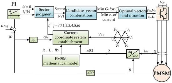
Figure 2.
Schematic of the proposed DV–MPC method.

Table 1.
Relationship between the worth functions and sectors.
Table 2.
Relationship between the vector combinations and sectors.
3.2. Current Coordinate System Establishment
It is assumed that the load model is linear with the back electromotive force. Then, the transformation between constant voltage vectors in αβ is an offline transformation, i.e., a linear transformation plus a translation [17]. Thus, the resulting current space vectors also form a hexagon. However, the hexagons of the current space vector are not centered on the origin of the complex plane and are time–varying.
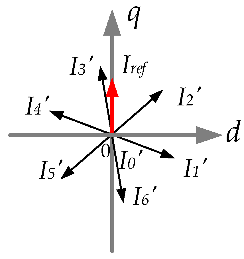
As shown in Figure 3, the reference current vector can be placed at the same starting point as the inverter current vector after the translation using (6).
where I is the current vector and I’ is the translated current vector.

Figure 3.
Current vector coordinate system.
3.3. Sector Determination
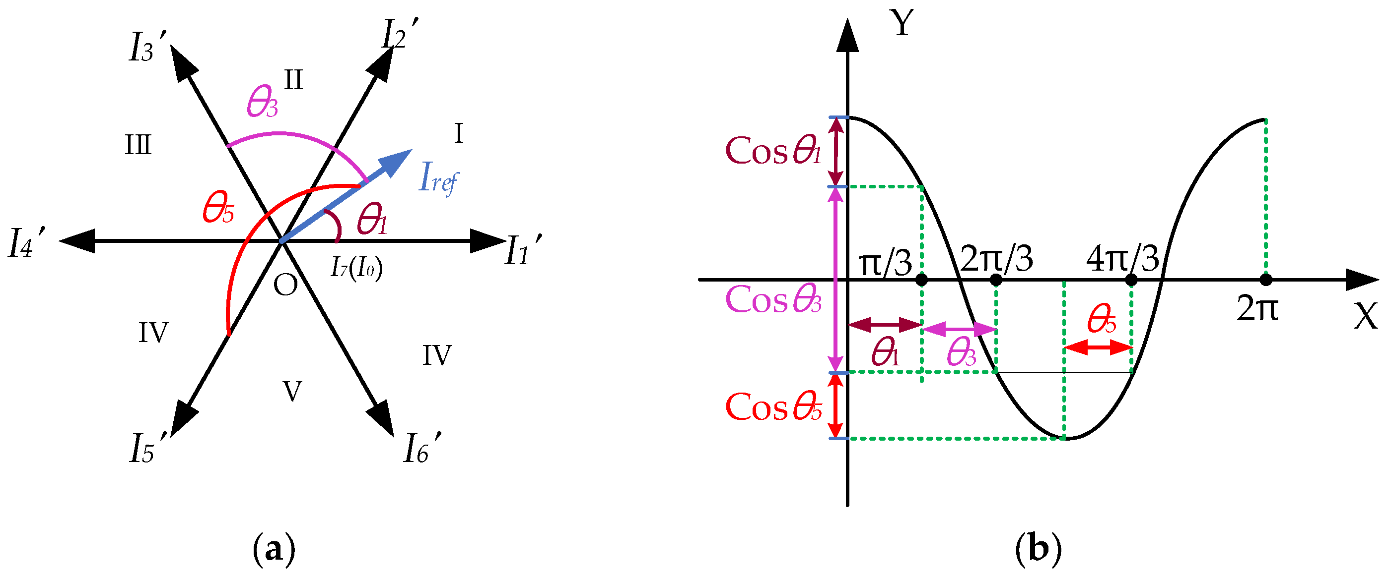
The positive direction of an arrow is indicated by its orientation. When projected in the opposite direction, the projection scale becomes negative. To alleviate the computational burden on the digital processor, the worth function can be defined using the following equation as the projection ratio (see Figure 4):
where Wj is the worth function of the jth vector, and where Idq is the dq−axis component.
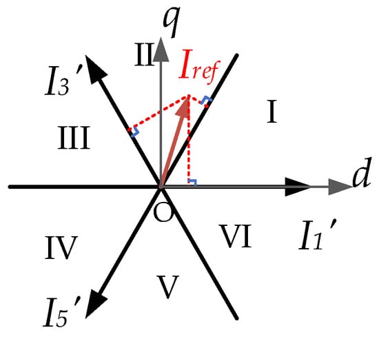
Figure 4.
Schematic of the sector determination.
Assuming the reference vector is in the second sector, the relative order of the worth functions for I1′, I3′, and I5′ are W3 > W1 > W5. Similarly, the relative order of the worth functions for the reference vector in other sectors can be determined. Therefore, it is only necessary to compute W1, W3, and W5 and compare their magnitudes to determine the sector in which the reference vector is located.
To prove the correspondence between each sector and the size of the worth function, consider a reference vector in the first sector as an example and compare the worth functions corresponding to I1′, I3′, and I5′ at this time. According to (7), the ratio of the projection of the reference current vector onto the active current vector Ij′ to the amplitude of Ij′ can be expressed using the following equation:
Due to the operating characteristics of the two–stage inverter, all six effective current vectors have the same magnitude at any given same time. Therefore, the magnitude of the worth function solely depends on the θi. From Figure 5a, it can be seen that when the reference current vector is located in the first sector, θ1 ∈ [0, π/3], θ3 ∈ [π/3, 2π/3], and θ5 ∈ [π, 4π/3]. By obtaining the specific range of θ1, θ3, and θ5, the magnitude relationships between cosθ1, cosθ3, and cosθ5 are shown in Figure 5b.
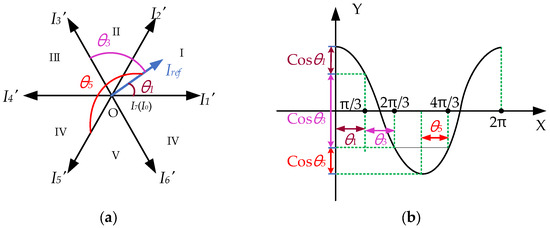
Figure 5.
Range diagrams using (a) θj, (b) cosθj.
It can be seen that the size relationship of Ij’ corresponding to the worth function is W1> W3 > W5. Similarly, when the reference current vector is located in other sectors, the magnitude relationship between the corresponding worth functions of Ij’ can be shown in the same way. Therefore, according to the size relationship of Wi, it is easy to determine the sector in which the reference voltage is located. The specific sector correspondence and the selected sector are shown in Table 1. With respect to Table 1, the sector in which the reference vector resides can be easily obtained through calculating and sorting the W1/3/5 amplitude values, thus further simplifying the calculation burden.
3.4. Vectors Selection and Action Time Calculation
According to the analysis in Section 2.2 and Figure 1b, there are five sets of candidate vector combinations for each sector as the position of the reference current vector is determined. The detailed vector selection is given in Table 2.
To determine the final selected vector group from the candidate vector set, the cost function defined by the square of l2 — norm is used [18]. The optimal vector combination is determined by finding the vector combination that minimizes the cost functions Gi for Ci:
where d1= t1/Ts and d2 = t2/Ts are the duty cycles of the corresponding vectors.
The vector duration time is found by minimizing the current ess using the following equations:
to deduce:
where,
3.5. Relationship of Action Time and Gate Signal
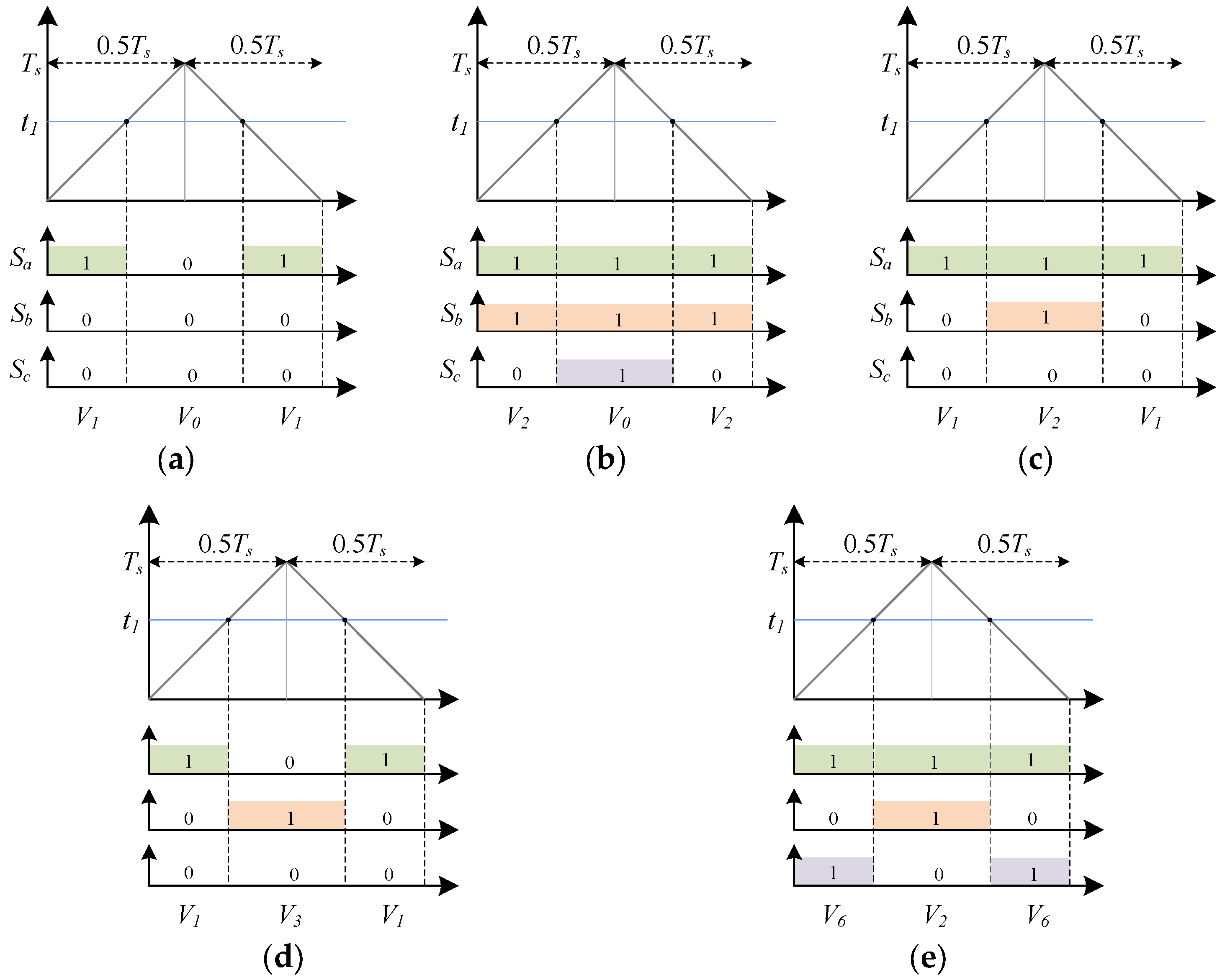
After obtaining the sector information from Section 3.3, the optimal vector is selected through the value function, and the action time of the corresponding vector is determined by Equations (11) and (12). Figure 6 illustrates the three–phase switching sequence in which the selected voltage vector is applied to the inverter in a specific order and action time, with the Sector I as an example. As shown in Figure 6, the corresponding switching sequence can be output within the corresponding time range within a control cycle through the comparison between the triangular carrier and the vector acting time. It is worth noting that for a combination of an effective vector and a zero vector, the switch sequence corresponding to V0 is (000) when the effective vector subscript is odd, otherwise it is (111).
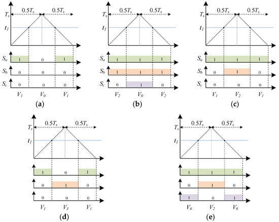
Figure 6.
The gate signal in the first sector as an example. (a) C1(V1, V0), (b) C2(V2, V0), (c) C3(V1, V2), (d) C4(V1, V3), (e) C5(V6, V2).
3.6. Process of the Proposed Method
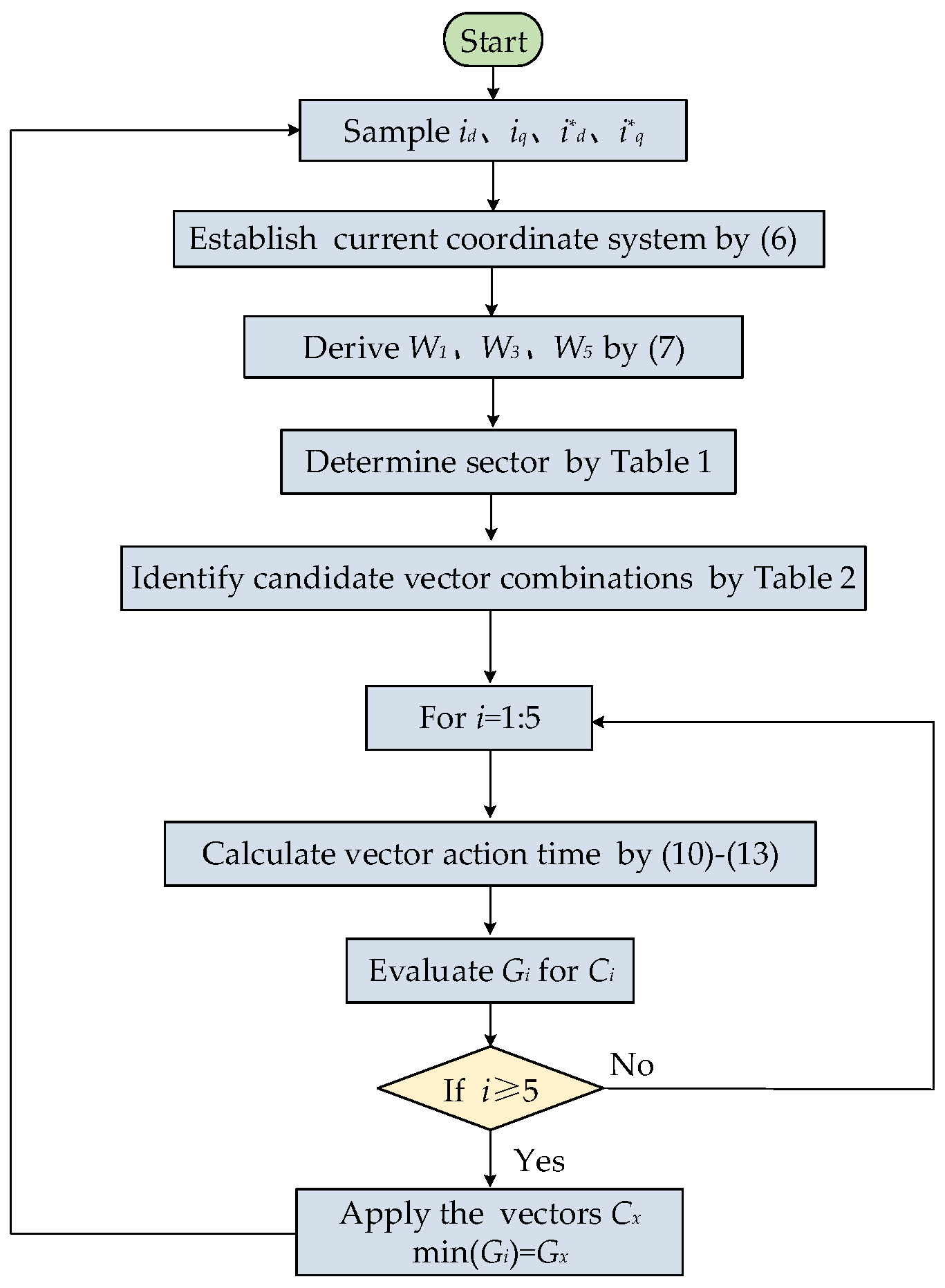
To sum up, the specific flow diagram of the proposed method is shown in Figure 7. Firstly, the d−q axis current is measured using this method, and the current coordinate system is established by combining the working principle of the inverter and the mathematical model of the motor. Then, the relationship of the three worth functions is obtained through (7), the sector where the reference current is located is determined in combination with Table 1 and Table 2, and five candidate vector combinations are determined. After that, solving (10)–(13) can derive the cost functions of each one of the five vector combinations. After that, the vector combination can be chosen to associate with the minimum cost function. Finally, according to Section 3.5, the switching state, switching time, and switching sequence corresponding to the selected vector can be applied to the inverter.

Figure 7.
The flow diagram of the proposed method.
4. Validation Results
To verify the effectiveness and benefits of the proposed DV–MPC method, the DV–MPC method introduced in Section 2 and the SV–MPC method is taken as the benchmark for comparison. A motor drive system including a two–level power inverter and a 2500 rpm PMSM model is built within the PLECS environment. The system parameters are shown in Table 3, where the sampling period of the control system is 50 μs.
Table 3.
Machine parameters.
4.1. Computational Time
To compare the computational complexity of the algorithms, a timer in PLECS is used to calculate the execution time of each algorithm in one control cycle using the following PC hardware: Intel 12th Gen Core i7–12700, 12–cores at 4.7 GHz, 16 GB RAM. The timer starts at the beginning of the calculation of the algorithm and ends when the calculation is complete. This measurement is repeated for 8000 control cycles, where the average execution time is recorded and listed in Table 4.
Table 4.
Execution time of the considered methods.
As shown in Table 4, the implementation of the DV–MPC algorithm in [14] requires 181.51 μs, while the proposed method only requires 169.28 μs. Compared to the DV–MPC algorithm in [14], the proposed method reduces the computation time by 6.74%. This reduction is due to the additional computational burden in the DV–MPC method, where the determination of sectors involves the use of arctangent functions. In contrast, the proposed method does not require trigonometric calculations, resulting in faster computation speed. It can be observed that the results obtained are in agreement with the theoretical results described in Section 3. The above results show that the computational complexity of the proposed DV–MPC method is lower than that of the traditional DV–MPC technique [14], which is due to the rapid selection of the optimal voltage vector based on the newly constructed vector selection table.
In addition, it also can be seen that compared with the SV–MPC method, the execution time of the proposed technique and the DV–MPC in [14] approach is increased. This is because the proposed technique and the DV–MPC in [14] approach involve the calculation of vector action time, which is also an essential problem to improve the steady–state performance of the SV–MPC method.
4.2. Dynamic Performance Comparison
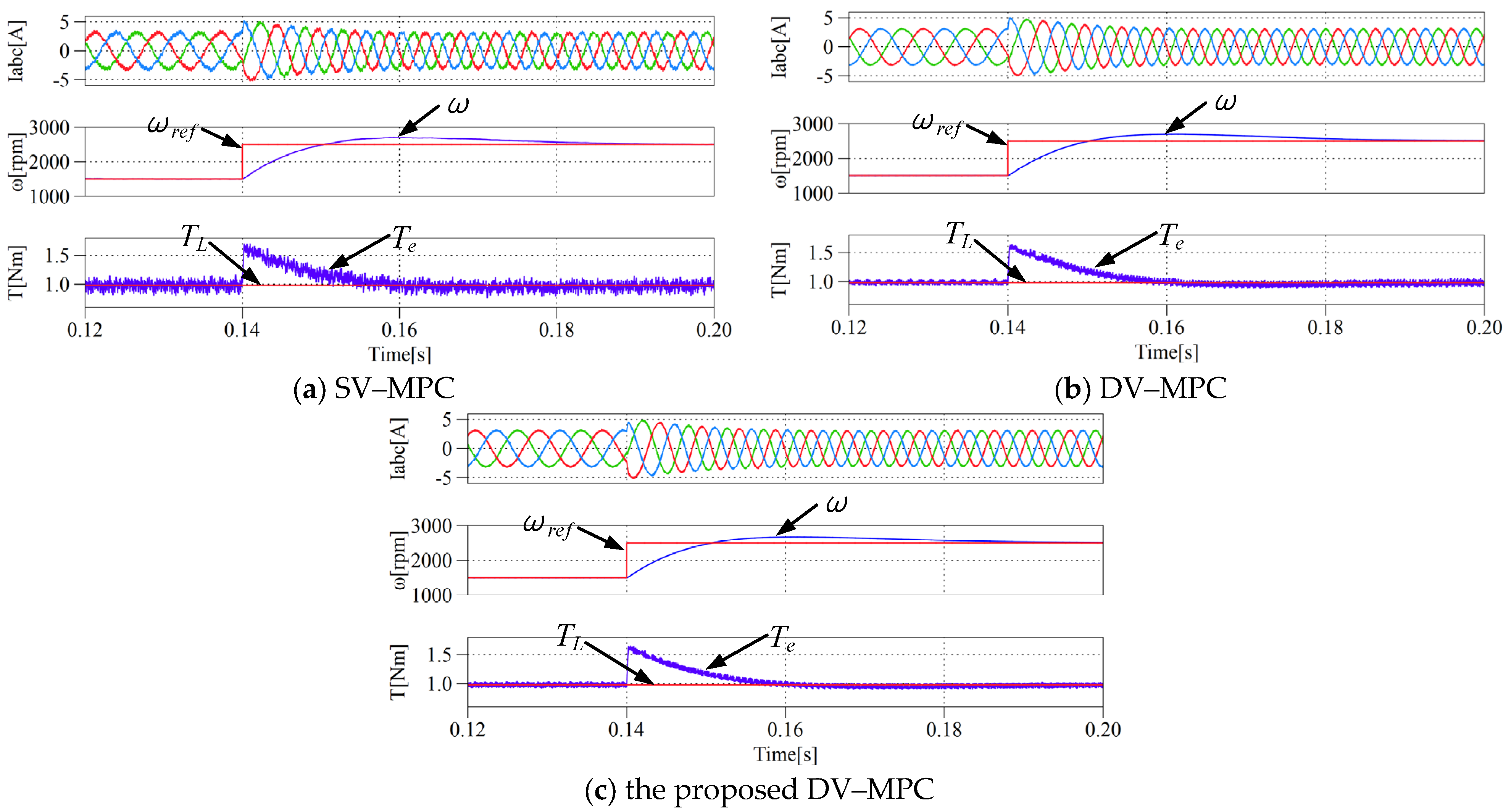
The transient characteristics of the step–rated speed for the proposed method were tested as depicted in Figure 8. Initially, the machine was started at a speed of 1500 rpm, followed by an immediate command of a step–rated speed reference at 2500 rpm when the time t = 0.14 s. Since the proposed method, DV–MPC technique in [14], and the SV–MPC approach adopt the same discrete load model, the proposed method and DV–MPC technique in [14] can precisely track the reference speed without exhibiting a noticeable overshoot, similar to the SV–MPC algorithm. Similarly, it can also be observed that, of the three methods, the proposed DV–MPC technique has the lowest current THD and the smallest torque ripple.
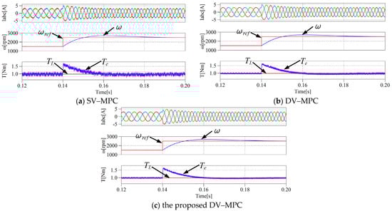
Figure 8.
System performance when the reference speed increases from 1500 rpm to the rated speed [14].
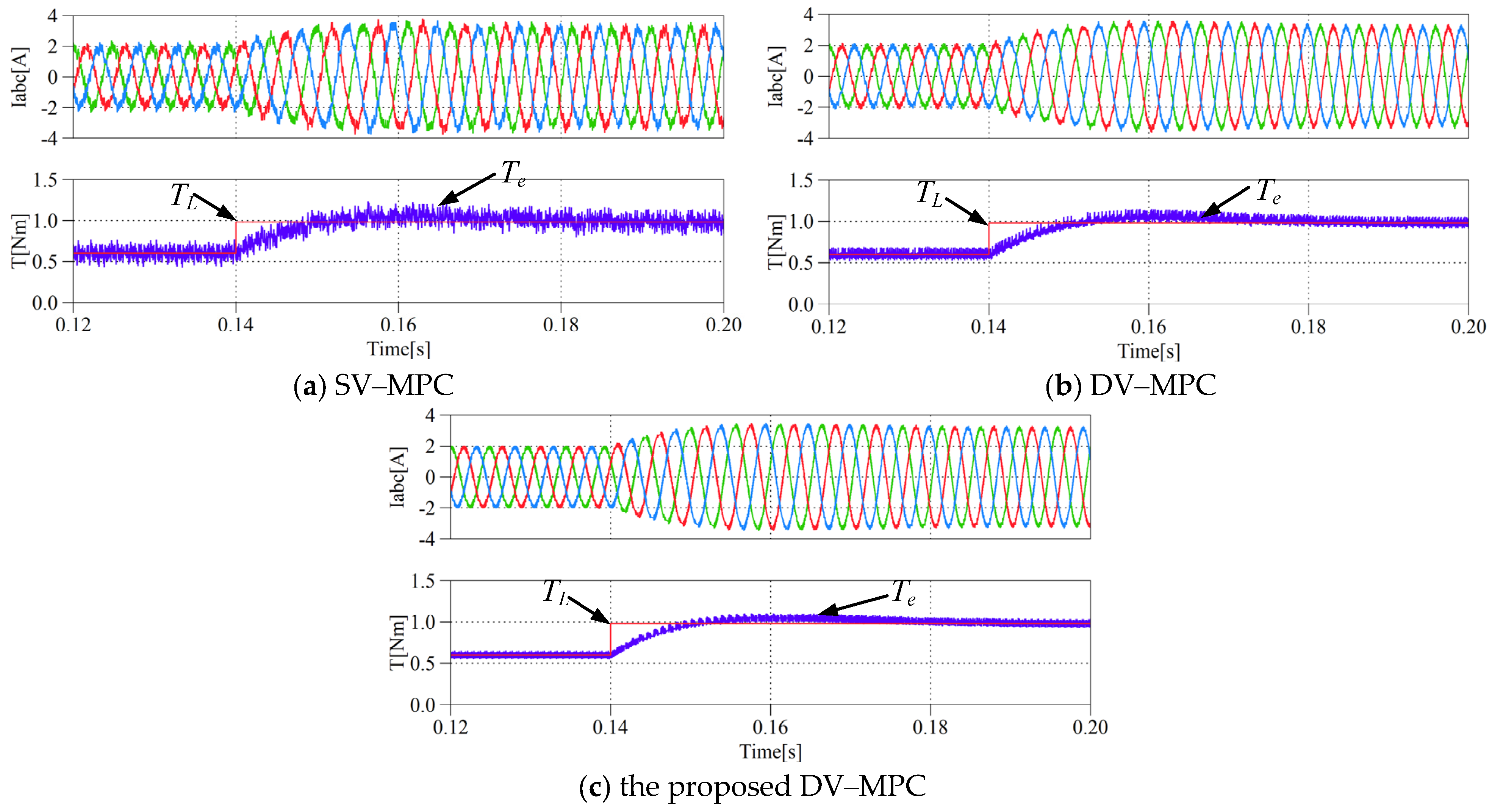
The transient behavior of the proposed control algorithm for a torque step was investigated, as shown in Figure 9. It is evident that the proposed method, as well as the DV–MPC method, demonstrates a rapid dynamic response, similar in speed to the SV–MPC algorithm. This result shows the equivalency of the proposed DV–MPC algorithm with the traditional method under this transient condition.
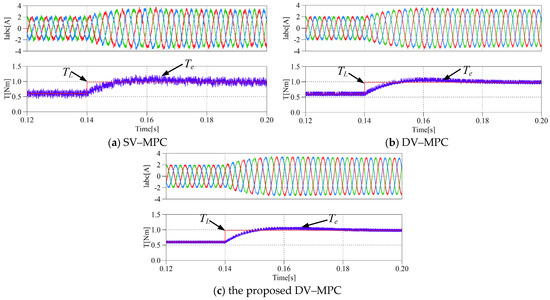
Figure 9.
System performance when the load torque increases from 0.6 Nm to the rated torque [14].
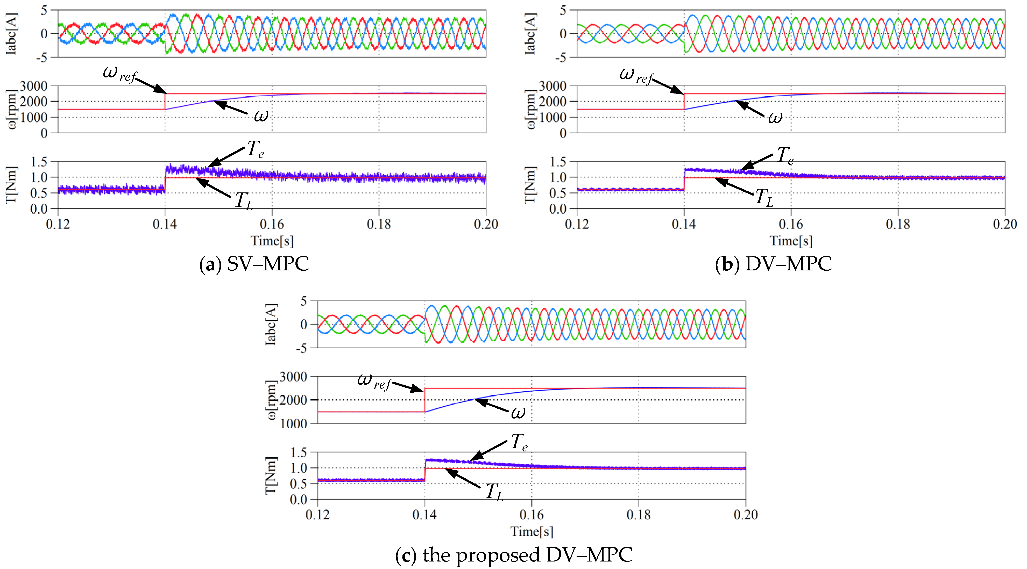
Figure 10 shows that when the load torque and the reference speed change at the same time, the three methods can quickly track their references. All three methods show strong robustness to external interference. The proposed DV–MPC method also shows reduced torque and current ripple, due to the superiority of vector selection of the proposed method. As shown in Figure 8, Figure 9 and Figure 10, because all three methods employ predictive control, each has a similar dynamic response. However, in terms of current ripple and harmonics, the proposed DV–MPC method has better steady–state performance than the SV–MPC technique and the DV–MPC method in [14].
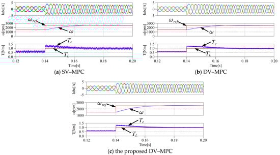
Figure 10.
System performance when the load torque increases from 0.6 Nm to the rated torque and the reference speed increases from 1500 rpm to the rated speed [14].
4.3. Steady–State Performance Comparison
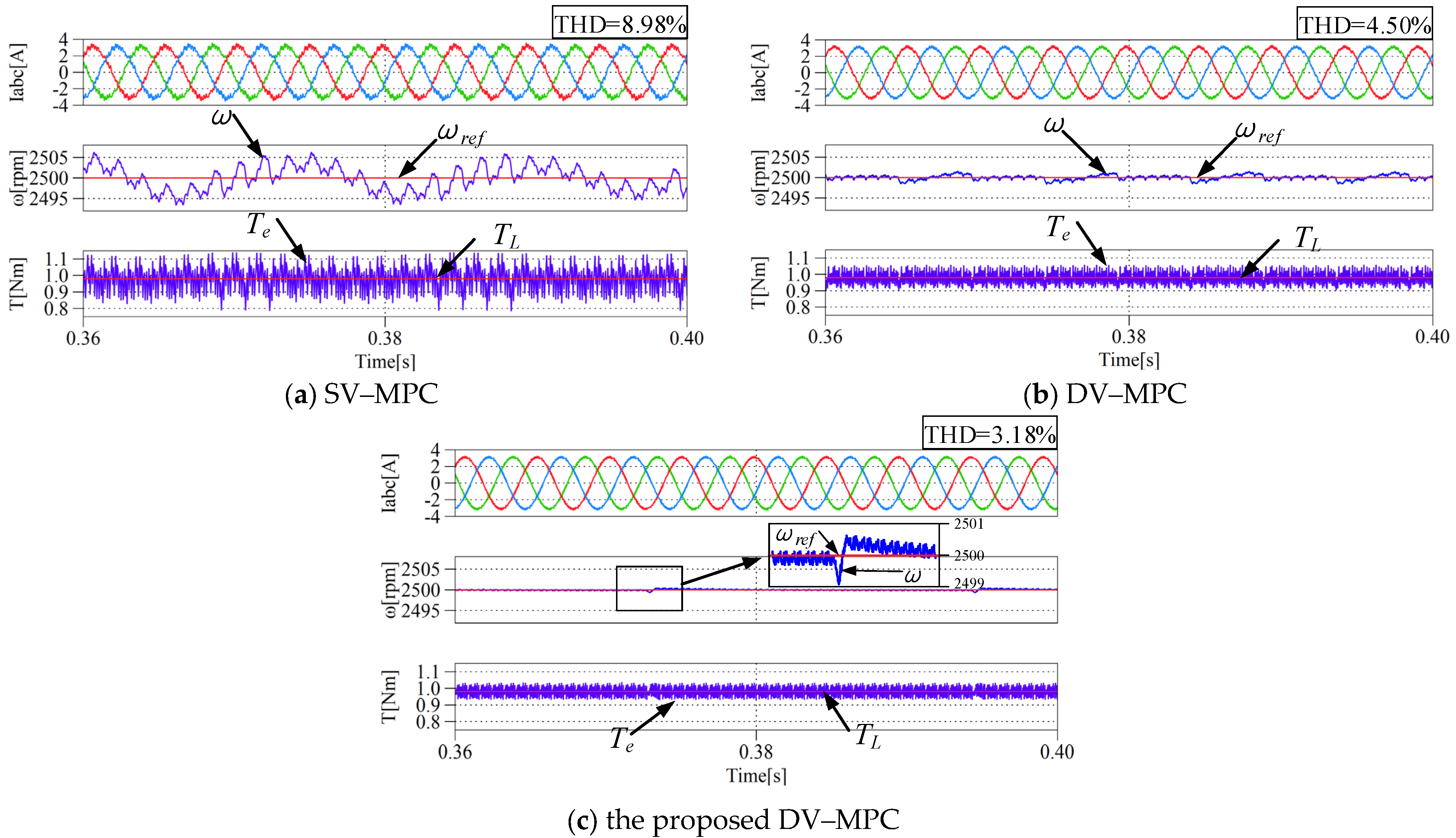
As shown in Figure 11a–c, a comparison of three methods was conducted for the steady–state performance of three–phase current, speed, and torque at rated power. It can be seen that compared with the SV–MPC method and DV–MPC technique in [14], the phase current, speed, and torque waveforms of the proposed DV–MPC method are significantly improved. This is due to the superiority of the proposed method in vector combination selection.

Figure 11.
System performance at the rated power [14].
In particular, from Figure 11, it can be seen that the SV–MPC method results in increased torque and speed ripple due to its action in only one vector per cycle, with ripple values of 14.56 rpm and 0.358 Nm, respectively, in this example. In the case of the DV–MPC method in [14], the speed ripple is 3.43 rpm, and the torque ripple is 0.16 Nm. In the proposed method, the speed ripple is 1.45 rpm, and the torque ripple is 0.10 Nm. It can be seen that the DV–MPC method significantly improves the steady–state performance compared to the SV–MPC technique. In the DV–MPC methods, the proposed method reduces speed ripple and torque ripple by 57.7% and 37.5%, respectively, compared to the DV–MPC method proposed in [14].
It also can be seen that the proposed method has a significantly lower current ripple compared to the SV–MPC method and DV–MPC method. Specifically, the current THD of the SV–MPC method is 8.98%, the current THD of the DV–MPC technique is 4.5%, and the current THD of the proposed approach is only 3.18%. The current THD for the proposed method is 64.6% lower compared to the SV–MPC method and 29.3% lower compared to the DV–MPC method in [14], as shown in Figure 11a–c.
The above results show that compared with the traditional SV–MPC method and DV–MPC technique in [14], the proposed DV–MPC approach has obvious improvement in current THD, torque ripple, and speed ripple. This benefits from the extension carried out by vector combination in the proposed method.
4.4. Discussion
A qualitative comparison of the common MPC methods is shown in Table 5. The evaluation criteria include the utilization of trigonometric functions, prediction horizon, and the dynamic performance (computational speed) and steady–state performance of the system. From Table 5, it can be seen that the SV–MPC method shows the best dynamic response, as it does not require vector action time allocation. However, its steady–state performance is poorer due to using only one switching state within a control period.
Table 5.
Evaluation of representative DV–MPC methods.
To improve the steady–state performance, the DV–MPC methods sacrifice some dynamic performance. For example, the DV–MPC method in [11] achieves superior steady–state performance but has very poor dynamic performance due to the requirement for 25 calculations per cycle. Other DV–MPC methods [12,13,14,15,16] reduce the prediction horizon by adopting the adjacent vectors. However, the restricted vector composition limits the vector synthetic range to active vectors and sector boundaries, lowering the steady–state performance.
Although requiring only three predictions [14], the DV–MPC technique exhibits a noticeable decrease in dynamic performance compared to other methods due to its reliance on trigonometric functions for sector determination. On the other hand, due to the superiority of vector combination selection, the proposed DV–MPC method presented in this paper demonstrates good performance in both dynamic and steady–state. It is worth noting that the results presented in this paper are obtained using a TMS320F28335 digital signal processor–in–the–loop within the PLECS environment.
5. Conclusions
In this paper, an improved DV–MPC method is proposed, adopting an optimal vector selection principle. By achieving the minimum number of calculation times for determining the optimal two vectors, the computational burden can be significantly reduced. At the same time, the DV–MPC method considers all the available combinations of the vectors, thus ensuring excellent control performance.
Compared to the existing DV–MPC methods in the literature, the proposed method can greatly improve the steady–state performance under the premise of reducing the computational burden. More specifically, compared to the previously reported DV–MPC method [14], the proposed method can reduce the torque ripple, speed ripple, and current THD by 37.5%, 57.7%, and 29.3%, respectively. The results have shown the advantages of the proposed DV–MPC method.
Author Contributions
Conceptualization, Z.H. and Q.W.; investigation and resources, Q.W. and Z.H.; writing—original draft preparation, Q.W. and X.X.; writing—review and editing, Z.H., P.W., and Q.W.; supervision, Y.X. and M.R.; funding acquisition, Z.H., P.W. and M.R. All authors have read and agreed to the published version of the manuscript.
Funding
This research was supported by Jiangxi Provincial Natural Science Foundation: 20224BAB214058, the National Natural Science Foundation of P.R. China (No. 52067015), ANID/FONDECYT Regular: 1220556, ANID/ANILLO: Centre for Multidisciplinary Research on Smart and Sustainable Energy Technologies for Sub–Antarctic Regions under Climate Crisis ANID/ATE220023, ANID/FONDAP: SERC 1522A0006, and the University of Nottingham: IRCF A7I502.
Data Availability Statement
The study did not report any data.
Conflicts of Interest
The authors declare no conflict of interest.
References
- Zhang, H.; Kou, B.; Zhang, L. Design and Analysis of a Stator Field Control Permanent Magnet Synchronous Starter–Generator System. Energies 2023, 16, 5125. [Google Scholar] [CrossRef]
- Zhang, X.; Yan, K.; Cheng, M. Two-Stage Series Model Predictive Torque Control for PMSM Drives. IEEE Trans. Power Electron. 2021, 36, 12910–12918. [Google Scholar] [CrossRef]
- Zhang, X.; Bai, H.; Cheng, M. Improved Model Predictive Current Control with Series Structure for PMSM Drives. IEEE Trans. Ind. Electron. 2022, 69, 12437–12446. [Google Scholar] [CrossRef]
- Rodriguez, J.; Garcia, C.; Mora, A.; Flores-Bahamonde, F.; Acuna, P.; Novak, M.; Zhang, Y.; Tarisciotti, L.; Davari, S.A.; Zhang, Z.; et al. Latest Advances of Model Predictive Control in Electrical Drives—Part I: Basic Concepts and Advanced Strategies. IEEE Trans. Power Electron. 2022, 37, 3927–3942. [Google Scholar] [CrossRef]
- Rodriguez, J.; Garcia, C.; Mora, A.; Davari, S.A.; Rodas, J.; Valencia, D.F.; Elmorshedy, M.; Wang, F.; Zuo, K.; Tarisciotti, L.; et al. Latest Advances of Model Predictive Control in Electrical Drives—Part II: Applications and Benchmarking With Classical Control Methods. IEEE Trans. Power Electron. 2022, 37, 5047–5061. [Google Scholar] [CrossRef]
- Harbi, I.; Rodriguez, J.; Liegmann, E.; Makhamreh, H.; Heldwein, M.L.; Novak, M.; Rossi, M.; Abdelrahem, M.; Trabelsi, M.; Ahmed, M.; et al. Model Predictive Control of Multilevel Inverters: Challenges, Recent Advances, and Trends. IEEE Trans. Power Electron. 2023, 38, 10845–10868. [Google Scholar] [CrossRef]
- Harbi, I.; Ahmed, M.; Hackl, C.M.; Rodriguez, J.; Kennel, R.; Abdelrahem, M. Low-Complexity Dual-Vector Model Predictive Control for Single-Phase Nine-Level ANPC-Based Converter. IEEE Trans. Power Electron. 2023, 38, 2956–2971. [Google Scholar] [CrossRef]
- Li, Z.; Xia, J.; Gao, X.; Guo, Y.; Zhang, X. Dual-Vector-Based Predictive Torque Control for Fault-Tolerant Inverter-Fed Induction Motor Drives with Adaptive Switching Instant. IEEE Trans. Ind. Electron. 2023, 70, 12003–12013. [Google Scholar] [CrossRef]
- Guazzelli, P.R.U.; Santos, S.T.C.A.D.; De Castro, A.G.; Pereira, W.C.D.A.; De Oliveira, C.M.R.; Monteiro, J.R.B.D.A.; De Aguiar, M.L. Decoupled Predictive Current Control with Duty-Cycle Optimization of a Grid-Tied Nine-Switch Converter Applied to an Induction Generator. IEEE Trans. Power Electron. 2022, 37, 2778–2789. [Google Scholar] [CrossRef]
- Guazzelli, P.R.U.; Santos, S.T.C.A.D.; De Almeida Monteiro, J.R.B.; De Aguiar, M.L. Model Predictive Control with Duty Cycle Optimization and Virtual Null Vector for Induction Generator with Six Switch Converter. IEEE J. Emerg. Sel. Topics Power Electron. 2023, 11, 1422–1431. [Google Scholar] [CrossRef]
- Zhang, Y.; Yang, H. Generalized Two-Vector-Based Model-Predictive Torque Control of Induction Motor Drives. IEEE Trans. Power Electron. 2015, 30, 3818–3829. [Google Scholar] [CrossRef]
- Zhang, Y.; Yang, H. Model Predictive Torque Control of Induction Motor Drives with Optimal Duty Cycle Control. IEEE Trans. Power Electron. 2014, 29, 6593–6603. [Google Scholar] [CrossRef]
- Li, X.; Sun, J.; Fan, M.; Yang, Y.; Xiao, Y. An Improved SVM-based Optimal Duty Cycle Model Predictive Current Control for PMSM. In Proceedings of the 2023 IEEE International Conference on Predictive Control of Electrical Drives and Power Electronics (PRECEDE), IEEE, Wuhan, China, 16–19 June 2023; pp. 1–5. [Google Scholar]
- Saeed, M.S.R.; Song, W.; Huang, L.; Yu, B. Double-Vector-Based Finite Control Set Model Predictive Control for Five-Phase PMSMs With High Tracking Accuracy and DC-Link Voltage Utilization. IEEE Trans. Power Electron. 2022, 37, 15234–15244. [Google Scholar] [CrossRef]
- Zhang, X.; Hou, B. Double Vectors Model Predictive Torque Control Without Weighting Factor Based on Voltage Tracking Error. IEEE Trans. Power Electron. 2018, 33, 2368–2380. [Google Scholar] [CrossRef]
- Chen, W.; Zeng, S.; Zhang, G.; Shi, T.; Xia, C. A Modified Double Vectors Model Predictive Torque Control of Permanent Magnet Synchronous Motor. IEEE Trans. Power Electron. 2019, 34, 11419–11428. [Google Scholar] [CrossRef]
- Garcia, C.F.; Silva, C.A.; Rodriguez, J.R.; Zanchetta, P.; Odhano, S.A. Modulated Model-Predictive Control with Optimized Overmodulation. IEEE J. Emerg. Sel. Topics Power Electron. 2019, 7, 404–413. [Google Scholar] [CrossRef]
- Karamanakos, P.; Geyer, T.; Kennel, R. On the Choice of Norm in Finite Control Set Model Predictive Control. IEEE Trans. Power Electron. 2018, 33, 7105–7117. [Google Scholar] [CrossRef]


Disclaimer/Publisher’s Note: The statements, opinions and data contained in all publications are solely those of the individual author(s) and contributor(s) and not of MDPI and/or the editor(s). MDPI and/or the editor(s) disclaim responsibility for any injury to people or property resulting from any ideas, methods, instructions or products referred to in the content. |
© 2023 by the authors. Licensee MDPI, Basel, Switzerland. This article is an open access article distributed under the terms and conditions of the Creative Commons Attribution (CC BY) license (https://creativecommons.org/licenses/by/4.0/).